
Working Paper 1506
Research Department
https://doi.org/10.24149/wp1506r1
Working papers from the Federal Reserve Bank of Dallas are preliminary drafts circulated for professional comment.
The views in this paper are those of the authors and do not necessarily reflect the views of the Federal Reserve Bank
of Dallas or the Federal Reserve System. Any errors or omissions are the responsibility of the authors.
Non-Renewable Resources,
Extraction Technology and
Endogenous Growth
Gregor Schwerhoff and Martin Stuermer

Non-Renewable Resources, Extraction Technology and
Endogenous Growth
*
Gregor Schwerhoff
†
and Martin Stuermer
‡
December 29, 2015
Revised: August 2019
Abstract
We document that global resource extraction has strongly increased with economic
growth, while prices have exhibited stable trends for almost all major non-renewable
resources from 1700 to 2018. Why have resources not become scarcer as suggested by
standard economic theory? We develop a theory of extraction technology, geology and
growth grounded in stylized facts. Rising resource demand incentivises firms to invest in
new technology to increase their economically extractable reserves. Prices remain
constant because increasing returns from the geological distribution of resources offset
diminishing returns in innovation. As a result, the aggregate growth rate depends partly
on the geological distribution of resources. For example, a greater average concentration
of a resource in the Earth's crust leads to more resource extraction, a lower price and a
higher growth rate on the balanced growth path. Our paper provides economic and
geologic microfoundations explaining why flat resource prices and increasing production
are reasonable assumptions in economic models of climate change.
Keywords: Non-renewable resources, endogenous growth, extraction technology
JEL Codes: O30, O41, Q30, Q43, Q54
*
The views in this paper are those of the authors and do not reflect the views of the Federal Reserve Bank of Dallas, the
Federal Reserve System or the World Bank. We thank Anton Cheremukhin, Thomas Covert, Klaus Desmet, Maik
Heinemann, Martin Hellwig, David Hemous, Charles Jones, Dirk Krüger, Lars Kunze, Florian Neukirchen, Pietro Peretto,
Gert Pönitzsch, Salim Rashid, Gordon Rausser, Paul Romer, Luc Rouge, Sandro Schmidt, Sjak Smulders, Michael Sposi,
Jürgen von Hagen, Kei-Mu Yi, and Friedrich-Wilhelm Wellmer for very helpful comments and suggestions. We also thank
participants at the Economic Growth Small Group Meeting at the NBER Summer Institute, AEA Annual Meeting, AERE
Summer Meeting, EAERE Summer Conference, SURED Conference, AWEEE Workshop, SEEK Conference, USAEE
Annual Meeting, SEA Annual Meeting, University of Chicago, UT Austin, University of Cologne, University of Bonn, MPI
Bonn, European Central Bank, and the Federal Reserve Bank of Dallas for their comments. We thank Mike Weiss for
editing. Navi Dhaliwal, Achim Goheer, Ines Gorywoda, Sean Howard and Emma Marshall provided excellent research
assistance. All errors are our own. An earlier version was published as a Dallas Fed Working Paper in 2015 and as a Max
Planck Institute for Collective Goods Working Paper in 2012 with the title “Non-renewable but inexhaustible: Resources in
an endogenous growth model."
†
Gregor Schwerhoff, Mercator Research Institute on Global Commons and Climate Change, gschwerhoff@worldbank.org.
‡
Martin Stuermer, Federal Reserve Bank of Dallas, Research Department, martin.stuerm[email protected].

1 Introduction
Economic intuition suggests that non-renewable resources like metals or fossil fuels become
scarcer and more expensive over time. However, our new data set for 65 resources from 1700
to 2018 disagrees. Not only has the production of non-renewables increased, but most of their
prices have exhibited non-increasing trends. This paper proposes an explanation: innovation
in extraction technology exploits a geological law where greater quantities of a resource are
found in progressively lower grade deposits. The result is increasing resource production at
non-increasing prices to meet growing global demand. Furthermore, it is this interaction
between technology and geology that co-determines the rate of long-run aggregate growth.
We document three stylized facts that support the mechanism of our model. First, the
Fundamental Law of Geochemistry (Ahrens, 1953) states that resources are log-normally
distributed in the Earth’s crust. This means greater quantities of a resource are locked in
lower grade deposits. Second, non-renewable resources are very abundant in the Earth’s
crust. However, only a small fraction called reserves is economically recoverable with current
extraction technology. Third, firms can increase reserves by investing in new technology but
there are diminishing returns in terms of accessing lower grade deposits.
We integrate a more realistic extraction sector into a standard lab-equipment model of
endogenous growth (Romer (1987, 1990) and Acemoglu (2002)).
1
Extraction firms observe
aggregate resource demand and invest in new extraction technology. This allows them to
increase their reserves and to extract the resource from lower grade deposits. They purchase
1
Besides the extractive sector, the model features a standard intermediate goods sector with goods and
sector-specific technology firms. The final good is produced from the intermediate good and the non-
renewable resource.
2
the technology from technology firms.
Technology firms invent new extraction technology because it is rivalrous. Each technol-
ogy is specific to deposits of particular grades. Most similar to this understanding of inno-
vation is Desmet and Rossi-Hansberg (2014), where non-replicable factors of production like
land provide the incentive for innovation despite perfectly competitive markets. Although it
becomes progressively harder to develop technologies for lower grade deposits, their resource
quantities increase exponentially. Thus the geological distribution of the resource offsets the
diminishing returns from technological development. The cost of technology per unit of the
resource and its price are constant over the long term.
On the balanced growth path, aggregate output and extraction grow at a constant rate,
whereas the resource price is constant. The three variables depend partly on the resource
distribution in the Earth’s crust. For example, a higher average geological concentration of
the resource leads to a higher rate of resource extraction, a lower price level and a higher
aggregate growth rate in equilibrium holding other factors constant. The rivalrous nature
of extraction technology implies that the extraction sector only exhibits constant returns to
scale and is not an engine of growth.
The interaction between resource distribution and extraction technology determines the
long-run rate of aggregate output growth along with the usual factors. This contrast with
conventional models that include a drag on growth driven by depletion and where this de-
pletion effect can be partially offset by the development of resource-saving technology or
substitution (see Nordhaus et al., 1992; Weitzman, 1999; Jones and Vollrath, 2002).
Based on geological and economic micro-foundations our model shows that constant re-
source prices and increasing extraction are reasonable long assumptions over the long term.
3
This is relevant to a growing literature studying the effects of fossil fuels on climate change
because it suggests that the transition towards clean energy will be more costly (Acemoglu
et al., 2012a; Golosov et al., 2014; Hassler and Sinn, 2012; van der Ploeg and Withagen,
2012; Acemoglu et al., 2019). Our model also suggests that demand side policies to curb
fossil fuel consumption are effective, because they would slow down innovation in extraction
technology. This is in contrast to the so called ”Green Paradox” , where an exhaustible stock
of fossil fuels incentivices firms to bring forward extraction when faced with demand side
policies (see Sinn, 2008; Eichner and Pethig, 2011; Van der Ploeg and Withagen, 2012). At
the same time, the availability of critical metals needed for the energy transition may not
face constraints. Continued increases in resource consumption might also also not raise the
risk of conflicts over resources (see Acemoglu et al., 2012b).
This paper challenges a literature that predicts greater resource scarcity with economic
development (see e.g. Stiglitz, 1974; Dasgupta and Heal, 1974; Solow and Wan, 1976; Nord-
haus et al., 1992; Aghion and Howitt, 1998; Jones and Vollrath, 2002; Groth, 2007). These
models rely on Hotelling’s (1931) characterization of optimal depletion: resource extraction
declines at a constant rate, while prices rise at the rate of interest. As a result, depletion
negatively affects output growth but can potentially be offset by substitution and techno-
logical change in resource efficiency. However, the literature also agrees that non-renewable
resources have neither become scarcer nor more expensive over time (see Nordhaus et al.,
1992; Krautkraemer, 1998; Livernois, 2009). This mismatch between theory and empirical
findings presents an open question (see Jones and Vollrath, 2002; Hassler et al., 2016).
Our paper contributes the interaction between geology and endogenous innovation in
extraction technology to the literature. We build on a small literature studying innovation in
4
extraction. In Rausser (1974) the non-renewable resource stock can increase due to learning-
by-doing, which allows for constant extraction and prices in a partial equilibrium model. Heal
(1976) argues that prices and extraction stay constant after a more costly but inexhaustible
“backstop technology”is reached. Cynthia-Lin and Wagner (2007) predict increasing resource
output and constant prices after adding exogenous technological change and heterogeneous
extraction costs to a model with an infinite resource. Tahvonen and Salo (2001) study
the transition from a non-renewable to a renewable energy resource with heterogeneous
extraction costs based on a growth model with learning-by-doing. Their model implies an
inverted U-shaped extraction and a U-shaped resource price path. Acemoglu et al. (2019)
study the role of fracking in the transition towards clean energy. In their setup, exogenous
technological change augments a constant flow of natural gas leading to a constant price.
The remainder of the paper is organized as follows. In section 2, we present empirical
evidence about the long-run trends of global resource extraction and prices based on a new
data-set. In section 3, we document stylized facts on geology and extraction technology.
Section 4 describes the main mechanism of our model, namely the interaction between ge-
ology and technology. Section 5 outlines the micro-economic foundations of the extractive
sector and its innovation process. Section 6 presents the growth model, and section 7 derives
theoretical results, which are discussed in section 8. Section 9 concludes and discusses policy
implications.
5

2 Long-Run Trends in Non-Renewable Resource Ex-
traction and Prices
We first present a new data-set of inflation adjusted resources prices and global production
from 1700 to 2018 for all major non-renewable resources.
2
2.1 Resource Extraction Has Strongly Increased
The extraction and consumption
3
of non-renewable resources strongly increased over the
past three hundred years. Figure 1 shows that global extraction rose from about 3.3 million
metric tons in 1700 to 21 billion metric tons in 2018. This is an increase by a factor of more
than 6000. About two thirds of the non-renewable resource production is driven by fossil
fuels, including crude oil, coal and natural gas, and the other third by metals and non-metals.
Global real GDP increased at a factor of about 190 over the same period, while real GDP
on a per capita basis multiplied by 15.
In per capita terms global resource extraction increased from roughly 5 to 3,000 kilograms.
A closer statistical examination confirms that the mine production of most non-renewable
resources exhibits significantly positive growth rates in the long term (see table 2 in the
appendix).
4
2
See Appendix 1 for data descriptions and sources.
3
Over the long term, extraction and consumption of resources are about equal, as stockholdings vary
over the business-cycle and are generally relatively small compared to consumption. In some cases, where
recycling is important, consumption could be higher. Our data is therefore a lower bound estimate for metals
and non-metals consumption.
4
These results also hold by-and-large for per capita production of the respective commodities over the
long run. Regressions results are available from the authors upon request.
6

Figure 1: World Extraction of 65 Non-Renewable Resources and World Real GDP, 1700-
2018. The total quantity of extracted non-renewable resources increased roughly in line with
world real GDP.
2.2 Non-Renewable Resource Prices Exhibit Non-Increasing Trends
Non-renewable resource prices exhibit strong fluctuations but follow mostly non-increasing
or even declining trends over the long term. Figure 2 presents an equally weighted and
inflation adjusted price index for 65 non-renewable resources, which shows a stable trend
over the long term. However, there is a significant uptick in crude oil and natural gas prices
since the 1970s, probably due to a structural break related to the changing roles of the Texas
Railroad Commission and oligopolistic behavior by OPEC (see Dvir and Rogoff, 2010).
We test the null hypothesis that growth rates of real prices are not significantly different
from zero. As the regression results in Table 3 in the appendix show, this null hypothesis
cannot be rejected. Real prices are mostly trend-less. Our evidence is in line with the
7

literature, see e.g. Krautkraemer (1998), Von Hagen (1989), Cynthia-Lin and Wagner (2007),
Stuermer (2018). The literature is certainly not definitive on price trends (see Pindyck, 1999;
Lee et al., 2006; Slade, 1982; Jacks, 2013; Harvey et al., 2010), but we conclude that prices
do generally not show increasing trends over the long term.
Figure 2: Inflation Adjusted Price Index for 65 Non-Renewable Resources (equally weighted),
1700-2018.
3 Stylized Facts
We lay out stylized facts about geology and extraction technology, which inform the main
mechanism of our model.
8

3.1 Non-Renewable Resources are Abundant in the Earth’s Crust
To better understand the interaction between geology and technological change, we first take
a closer look at the abundance and distribution of non-renewable resources in the Earth’s
crust.
We update and extend a data-set by Nordhaus (1974) on the abundance (or estimated
total quantity) of mineral non-renewable resources in the Earth’s crust. Table 1, second
column, shows that the crustal abundance of major non-renewable resources is substantial.
5
The fourth column shows annual mine production, which is several orders of magnitude
smaller than the quantities in the Earth’s crust. If production stayed constant, resources
are basically infinite as current extraction could continue for millions or billions of years
depending on the resource (see table 4 in the appendix).
A more realistic assumption is that extraction continues to grow exponentially at current
rates. In this case, production could still be sustained for a couple of hundred to a thousand
years if there is continued technological progress, as column 4 in table 1 illustrates. This is
still close enough to infinity for all practical economic purposes. Note also that the Earth’s
crust makes up less than one percent of the Earth’s mass. There are hence more non-
renewable resources in other layers of the Earth.
Hydrocarbons are quite abundant in the Earth’s crust. Even though reserves of conven-
tional oil resources – the highest grade fossil fuel – may be exhausted someday, deposits of
unconventional oil, natural gas, and coal, which could substitute for conventional oil in the
long run, are plentiful in the Earth’s crust. These results are in line with numerous stud-
5
9

ies that conclude that fossil fuels will last far longer than many expect (see Aguilera et al.
(2012), Rogner (1997) and Covert et al. (2016)).
Crustal
Abundance/ Reserves/
Crustal Annual Annual Annual
Abundance Reserves Output Output Output
(Bil. mt) (Bil. mt) (Bil. mt) (Years) (Years)
Aluminum 1,990,000,000
e
30
b1
0.06
a
491 42
1
Copper 1,510,000
e
0.8
b
0.02
b
483 26
Iron 1,392,000,000
e
83
b2
1.2
a
580 39
2
Lead 290,000
e
0.1
b
0.005
b
1,099 16
Tin 40,000
e
0.005
b
0.0003
b
1,405 14
Zinc 2,250,000
e
0.23
b
0.013
b
668 14
Gold 70
e
0.00005
b
0.000003
b
925 15
Coal
3
}
511
d
3.9
d
}
63
c
Crude Oil
4
15,000,000
f
241
d
4.4
d
558 41
c
Nat. Gas
5
179
d
3.3
d
34
c
Notes: We have used the following average annual growth rates of production from 1990 to 2010: Aluminum: 2.5%, Iron: 2.3%,
Copper: 2%, Lead: 0.7%, Tin: 0.4%, Zinc: 1.6%, Gold: 0.6%, Crude oil: 0.7%, Natural gas: 1.7%, Coal: 1.9%, Hydrocarbons:
1.4%.
1
Data for bauxite,
2
data for iron ore,
3
includes lignite and hard coal,
4
includes conventional and unconventional oil,
5
includes conventional and unconventional gas,
6
all organic carbon in the earth’s crust. Sources:
a
U.S. Geological Survey
(2016),
b
U.S. Geological Survey (2018),
c
British Petroleum (2017),
d
Federal Institute for Geosciences and Natural Resources
(2017),
e
Perman et al. (2003),
f
Littke and Welte (1992).
Table 1: Availability of selected non-renewable resources in years of production left in the
reserve and crustal mass assuming an exponentially increasing annual mine production (based
on the average growth rate over the last 20 years).
Of course, extraction of most of these resource quantities in the Earth’s crust is impos-
sible or extremely costly with current technology. Only a small fraction is proven to be
economically extractable with current technology. This fraction is defined as reserves (see
U.S. Geological Survey (2018)). The term “economic” implies that firms established prof-
itable extraction under defined investment assumptions with reasonable certainty. Table 1,
column three, shows that reserves are relatively small compared to their crustal abundance.
They amount to only a couple of decades of current extraction (see column six).
10

Figure 3: Non-Renewable Resource Flows.
Note: This is a stylized version of the official Resource/Reserve Classification System for Minerals as used by the U.S. Geological
Survey (see U.S. Geological Survey (2018)).
The boundary between reserves and other occurrences in the earth’s crust is dynamic due
to technological change and exploration. Figure 3 shows how resources are classified as either
reserves or other occurrences in the Earth’s crust.
6
As reserves deplete through extraction,
firms explore new deposits and develop new technology to convert other occurrences into
reserves. This allows firms to continue extraction. The extracted resource becomes either
part of the capital stock, discharges after utilization into landfills or the atmosphere.
3.2 Non-Renewable Resources are Log-Normally Distributed in
the Earth’s Crust
Non-renewable resources are not uniformly concentrated in the earth’s crust. Variations in
the geochemical processes have shaped the characteristics of non-renewable resource occur-
6
Please note that we have left out a major category, the reserve base, to ease understanding. The reserve
base encompasses those parts of the resource in the earth’s crust that have a reasonable potential for becoming
economically available within planning horizons beyond those that assume proven technology and current
economics (see U.S. Geological Survey (2018))
11
rences in the Earth’s crust over billions of years. Deposits differ in their geological character-
istics along many dimensions, for example, ore grades, thickness and depths. We focus on ore
grade, as this is the most important characteristic. Some deposits are highly concentrated
with a specific resource (high grade, close to 100 percent ore grade), and other deposits are
less so (low grade, close to 0 percent ore grade). The grade distinguishes the difficulty of
extraction, where a low grade is very difficult.
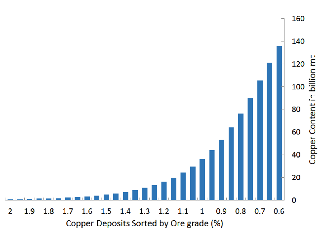
Figure 4: Grade-quantity distribution of copper in the Earth’s crust. The total copper
content increases, as the ore grades of copper deposits decline. The x-axis has been reversed
for illustrative purposes. Source: Gerst (2008).
The fundamental law of geochemistry (Ahrens (1953, 1954)) states that each chemical
element exhibits a log-normal grade-quantity distribution in the Earth’s crust, postulating a
decided positive skewness. Hence, the total resource quantity in low grade deposits is large,
while the total resource quantity in high grade deposits is relatively small. The reason for
this is that low grade deposits have a far larger volume of rock than high grade deposits. For
example, figure 4 shows that the total copper content increases, as the ore grades of copper
12
deposits in the Earth’s crust decline.
While a log-normal distribution for the distribution of certain resources is the text-book
standard assumption in geochemistry, this literature continues to develop, especially regard-
ing very low concentrations of metals, which might be mined in the distant future. For
example, Skinner (1979) and Gordon et al. (2007) propose a discontinuity in the distribution
due to the so-called “mineralogical barrier,” the approximate point below which metal atoms
are trapped by atomic substitution.
Gerst (2008) concludes in his geological study of copper deposits that he can neither
confirm nor refute this hypotheses. However, based on worldwide data on copper deposits
over the past 200 years, he finds evidence for a log-normal relationship between copper
production and ore grades. Mudd (2007) analyzes the historical evolution of extraction and
grades of deposits for different base metals in Australia. He also finds that production has
increased at a constant rate, while grades have consistently declined.
We conclude that there remains uncertainty about the geological distribution, especially
regarding hydrocarbons with their distinct formation processes. However, it is reasonable to
assume that non-renewable resources are distributed according to a log-normal relationship
between the grade of its deposits and its quantity based on geochemical theory and evidence.
3.3 Diminishing Returns to Innovation in Extraction Technology
Empirical evidence suggests that technological change affects the extractable ore grade with
diminishing returns (see Lasserre and Ouellette, 1991; Mudd, 2007; Simpson, 1999; Wellmer,
2008). For example, Radetzki (2009) and Bartos (2002) describe how technological changes
13

in mining equipment, prospecting and metallurgy have gradually enabled the extraction of
copper from lower grade deposits. The average ore grades of copper mines have decreased
from about twenty percent 5,000 years ago to currently below one percent (Radetzki, 2009).
Figure 5 illustrates this development using the example of global copper mines from 1800 to
2000. Mudd (2007) and Scholz and Wellmer (2012) come to similar results for different base
metal mines in Australia and for copper mines in the U.S, respectively.
Figure 5: The historical development of average ore grades of copper mines in the world
suggests diminishing returns of technological change on extractable ore grades. The y-axis
has been reversed for illustrative purposes. Source: Gerst (2008)
However, Figure 5 also shows that decreases in grades have slowed as technological de-
velopment progressed. Under the reasonable assumption that global real R&D spending
in extraction technology and its impact on technological change has stayed constant or in-
creased over the long term, there are decreasing returns to R&D in terms of making mining
from deposits of lower grades economically feasible.
14
We observe similar developments for hydrocarbons. Using the example of the offshore oil
industry, Managi et al. (2004) finds that technological change has offset the cost-increasing
degradation of resources. Crude oil has been extracted from ever deeper sources in the Gulf of
Mexico. Furthermore, technological change and high prices have made it profitable to extract
hydrocarbons from unconventional sources, such as tight oil or oil sands (International Energy
Agency, 2012).
Overall, we conclude that the long-run data suggests that there are no constant returns
from technological change in resource extraction in terms of ore grades. Historical evidence
rather suggests diminishing returns to technological development.
4 The Interaction Between Geology and Technology
The stylized facts highlighted the importance for understanding the interaction between
geology and technology in the extractive sector. In the following, we describe the key as-
sumptions which we make based on these stylized facts. We point out that there are offsetting
effects between geology and technology, which can lead to constant returns from technological
development in terms of new reserves.
4.1 Geological Function
We approximate the log-normal distribution of non-renewable resources in the Earth’s crust
by an increasing relationship between grade and quantity. The geological function (see also
15

Figure 6) takes the form:
R(O) =
δ
O
, δ ∈ R
+
, O
?
∈ (0, 1) . (1)
We define the grade O of a deposit as the average concentration of the resource. Parameter
δ controls the curvature of the function. If δ is high, the total quantity of the non-renewable
resources is large. For example, iron is relatively abundant with an average concentration of
5% in the Earth’s crust. A low δ indicates a relatively small quantity of the non-renewable
resource in the crustal mass. One example is gold with an average concentration of 0.001%.
The functional form implies that the resource quantity goes to infinity as the grade
approaches zero. Although we recognize that non-renewable resources are ultimately finite
in supply, we follow Nordhaus (1974) in his assessment that non-renewable resources are so
abundant in the earth’s crust that “the future will not be limited by sheer availability of
important materials” given technological change. Our assumption compares to households
maximizing over an infinite horizon.
16

1
O
?
O
?0
0
R
T ech
S(O
?0
)
Deposits Sorted from High to Low Ore Grades O
Resource Quantity R
Figure 6: Geological function: Deposits of lower grade O entail a higher resource quantity
R. The x-axis has been reserved for illustrative purposes and goes from high grades to low
grades. A new technology shifts the extractable grade from O
?
to O
?0
. The resulting flow
of new reserves is R
T ech
and indicated by the dark shaded area. The accumulated reserves
from the development of all technologies is S(O
?0
) (see light and dark shaded area).
Technological development makes extraction from lower grades possible and converts
deposits into reserves. For example, a new technology shifts the extractable deposits from
grade O
?
down to grade O
?0
. The cut-off grade O
?
indicates the lowest grade that firms
can extract with the new technology level. This technological change adds resources to the
reserves that are equal to: R
T ech
=
R
O
?
O
?0
R(O
?
)dO
?
, δ ∈ R
+
, O
?
∈ (0, 1) . The total amount
of resources converted to reserves due to technological change over the entire time horizon
[O
?0
, 1) is:
S(O
?0
) =
Z
1
O
?0
δ
O
?
dO = −δln(O
?0
), δ ∈ R
+
, O
?
∈ (0, 1) (2)
17
4.2 Diminishing Returns to Technology
We accommodate the diminishing returns of technological change by an extraction technology
function, which maps the state of the technology N
R
onto the extractable grade O
?
of the
deposits (see figure 7):
O
?
(N
R
) = e
−µN
R
, µ ∈ R
+
N
R
∈ (0, ∞) . (3)
The grade O
?
is the lowest grade that firms can extract with technology level N
R
. Tech-
nological change, N
R
, expands the range of grades that can be extracted. The extractable
grade is a decreasing convex function of technology implying decreasing marginal returns.
The curve in Figure 7 starts with deposits of close to a 100 percent ore grade, which rep-
resents the state of the world several thousand years ago. For example, humans picked up
copper in pure nugget form in Cyprus and beat it to the desired form, given its malleability
(see Radetzki, 2009). However, the quantity of copper that is in these high grade deposits
is relatively small. With technological change lower grade deposits became available, e.g.
today copper is mined from ore that contains below one percent of copper. The quantities
of copper contained in these deposits is much larger than in the high grade deposits.
18

1
0.8
0.6
0.4
0.2
0
Technology Level N
R
Deposits Sorted from High to Low Ore Grades O
Figure 7: The extraction technology function assumes diminishing returns to technological
development in terms of grades. The y-axis has been reserved for illustrative purposes.
The curvature parameter of the extraction technology function is µ. If, for example, µ
is high, the average effect of new technology on converting deposits to reserves in terms of
grades is relatively high.
4.3 Marginal Effect of Extraction Technology on Reserves
We show that the interaction of the geological and technology function produces a linear
relationship between technological development and reserves. Figure 8, Panel A, depicts
the technology function. Two equal steps in advancing technology from 0 to N and from
N to N
0
, lead to diminishing returns in terms of extractable ore grades O
?
and O
?0
, where
O
?0
− O
?
≺ O
?
.
Panel B shows equation 2, which is the integral of the geological function. The figure
presents how the different advances in extractable ore grades O
?
and O
?0
map into equal
19

increases in the accumulated reserve levels S and S
0
, where S
0
− S = S.
Figure 8: The interaction between the extraction technology function (Panel A) and the
accumulated geological function (Panel B) leads to a linear relationship between technology
level N
R
and reserves S (Panel C). Note that the y-axis in panel A and the x-axis in panel
B have been reversed for illustrative purposes.
Finally, Panel C summarizes how the extraction function and the accumulated geological
function offset each other and lead to a linear relationship between the technology level and
the reserve level.
Proposition 1 Reserves S increase proportionally to the level of extraction technology N
R
:
20

S(O
?
(N
Rt
)) = δµN
Rt
.
The marginal effect of new extraction technology on reserves equals:
dS(O
?
(N
Rt
))
dN
R
= δµ .
The intuition is that two offsetting effects cause this result: (i) the resource is geologically
distributed such that it implies increasing returns in terms of new reserves as the grade of
deposits decline; (ii) new extraction technology exhibits decreasing returns in terms of making
lower grade deposits extractable.
As the natural log in the accumulated geological function and the natural exponent in the
technology function cancel out, there is a linear relationship between the state of technology
N
R
and the total quantity of the resource converted into reserves S.
Proof of Proposition 1
S(O
?
(N
Rt
)) = −δ ln(O
?
(N
Rt
))
= −δ ln(e
−µN
Rt
)
= µδN
Rt
2
The equations in Proposition 1 depend on the shapes of the geological function and the
technology function. If the respective parameters δ and µ are high, the marginal return on
21

new extraction technology will also be high.
The constant marginal effect of technology on new reserves is a first approximation and
we allow for wide parameter spaces for the functional forms of the underlying functions. If
the technology function did not assume decreasing returns in terms of lower ore grades but
constant returns, this would result in an increasing marginal effect of technology on new
reserves. We discuss other function forms in section 8.
5 The Extractive Sector
We now describe the micro-foundations of the extractive sector and firms’ incentives to
develop technologies. Our extractive sector includes two types of firms: extraction and tech-
nology firms. Extraction firms buy technology from technology firms and extract the resource
from deposits of declining grades, while the latter innovate and produce extraction technol-
ogy.
7
Both types of firms know fully about the geological distribution and the technology
function.
5.1 Extraction Firms
We consider a large number of infinitely small extraction firms. They operate in a fully
competitive sector where demand for the non-renewable resource, a homogenous good, is
given.
8
7
To ease comparison, the extractive sector is constructed in analogy to the intermediate goods sector in
Acemoglu (2002).
8
We assume that the firm level production functions exhibit constant returns to scale, so there is no loss
of generality in focusing on aggregate production functions. We assume a fully competitive sector, because
we model long-run trends. Historically, producer efforts to raise prices were only successful in some non-oil
commodity markets in the short run, as longer-run price elasticities proved to be high (see Radetzki, 2008;
Herfindahl, 1959; Rausser and Stuermer, 2016). Similarly, a number of academic studies discard OPEC’s
22

Firms can hold reserves S. Reserves are defined as non-renewable resources in under-
ground deposits that can be extracted with grades-specific technology (or machine varieties)
at a constant extraction cost φ > 0. The marginal extraction cost for non-reserves is infinitely
high, φ = ∞. Firms’ reserves
˙
S evolve according to:
˙
S
t
= −R
Extr
t
+ R
T ech
t
, S
t
≥ 0, R
T ech
t
≥ 0, R
Extr
t
≥ 0. (4)
Firms can extract the resource from its reserves using grade-specific technology, a flow
that we denote as R
Extr
t
. Machines fully depreciate after use. However, firms can also expand
the quantity of their reserves by investing in new grades-specific technology, a flow denoted
as R
T ech
t
.
Extraction firms can purchase the new technologies from sector-specific technology firms
at price χ
R
. A new grades-specific technology allows firms to claim ownership of all non-
renewable resources in the related deposits. Firms declare these deposits their new reserves.
In our setup, reserves are a function of geology and extraction technology. They are
comparable to working capital in the spirit of Nordhaus (1974), as they are inventories of
resources in the ground that can be used as input to production. To put it differently, the
non-renewable resource is not defined as a fixed, primary factor but as a production factor
produced by technological change.
Due to the combination of constant returns to technological change in terms of new re-
serves (Proposition 1) and the assumption of grade-specific technology leads, Firms’ new
ability to raise prices over the long term (see Aguilera and Radetzki, 2016, for an overview). This is in line
with historical evidence that OPEC has never constrained members’ capacity expansions, which would be a
precondition for long-lasting price interventions (Aguilera and Radetzki, 2016)
23

reserves are a function of technological change
˙
N, the geological parameter δ and the tech-
nological parameter µ:
9
R
T ech
t
= δµ
˙
N
R
. (5)
This production function for reserves exhibits only constant returns to scale, which implies
that the social value of an innovation is equal to the private value. As R&D lifts resource
scarcity, future innovations are not reduced in profitability. No positive or negative spill-overs
occur in our model.
In our setup, extraction firms are basically like car producers, facing a marginal cost
curve and producing what is demanded at a given price. Firms only maximize current
profits, which are a function of the revenue received from selling the resource, extraction
cost and investment in new technologies to expand reserves:
π
E
R
= p
R
R
Extr
− φR
Extr
− χ
R
δµ
˙
N
R
, (6)
5.2 Technology Firms in the Extractive Sector
Sector-specific technology firms j invent patents for new varieties of grades-specific extrac-
tion technology (or machines). We assume that there is free entry of technology firms into
research. Technology firms observe the demand for grades-specific machine varieties by the
extraction firms. The innovation possibilities frontier, which determines the creation of new
technologies takes the form:
10
9
Please see Appendix 1.3 for the derivation of this equation.
10
We assume in line with Acemoglu (2002) that there is no aggregate uncertainty in the innovation process.
There is idiosyncratic uncertainty, but with many different technology firms undertaking research, equation
7 holds deterministically at the aggregate level.
24

˙
N
R
= η
R
M
R
. (7)
Each technology firm can spend one unit of the final good for R&D investment M at
time t to generate a flow rate η
R
> 0 of new patents, respectively. The cost of inventing a
new machine variety is
1
η
. Each firm can invent only one new machine variety at a time in
line with Acemoglu (2002).
A firm that invents a new extraction machine receives a perpetual patent. The patent
grants the firm the right to build the respective machine at a fixed marginal cost ψ
R
> 0.
However, the knowledge about building the machine diffuses to all technology firms and can
be used to invent new machine varieties for lower ore grades. The economy starts at the
initial technology level N
R
(0) > 0.
Based on the patent, firms produce a machine, which makes a particular deposits of lower
grades O extractable and can only be used for this specific geological formation. The use
of a machine by one extraction firm prevents other extraction firms from using it because
of this feature. Once these deposits are extracted, new machine varieties must be invented.
Technology is hence rivalrous in the context of extracting non-renewable resources.
11
As each machine variety is specific to deposits of certain grades, only one machine is build
and sold per variety. As a consequence, each technology firm stays in the market for only
one time period. The value of a technology firm that discovers a new machine depends on
instantaneous profits:
11
This is in contrast to the intermediate goods sector, where technology is non-rivalrous.
25
V
R
(j) = π
R
(j) = χ
R
(j)x
R
(j) − ψ
R
x
R
(j) , (8)
The present value of a patent is the difference between the machine price χ
R
(j) and the cost
to produce a machine ψ
R
times the number of produced machines x
R
(j) = 1.
This formulation allows us to boil down a dynamic optimization problem to a static one.
It makes the model solvable and computable. At the same time, the model stays rich enough
to derive meaningful theoretical predictions about the relationship between technological
change, geology and economic growth.
5.3 Timing
Figure 9 illustrates the timing in our model. At the start of period t, the aggregate produc-
tion sector demands resources from the extraction firms. The extraction firms request new
machine varieties from the technology firms to access deposits of lower grades.
In the early period of t, technology firms observe this demand. They invest into new
machines that are specific to the grades of the respective deposits. Firms enter the market
until the value of entering, namely profits, equals market entry cost, which is the cost to
invent a new technology. Each technology firm obtains a patent for their newly developed
machine variety, produces one machine based on the patent and sells it to the extraction
firms. The knowledge about the machine directly diffuses to the other firms.
In the mid-period of t, extraction firms convert deposits to reserves based on the new
machines. In the later period of t, extraction firms extract the resource and sell it to the
final good producers.
26

Start period t:
Extracting firms
observe resource
demand
R
D
and
demand new
machines
˙
N
Early period t:
Technology
firms enter the
market, develop
and sell new
machines
˙
N
Mid period t:
Extracting
firms convert
deposits
into reserves
Late period t:
Extracting
firms extract
R and sell it
to aggregate
producer
Figure 9: Timing and Firms’ Problem
6 The Endogenous Growth Model
To study the aggregate effects of the interaction between geology and extraction technology,
we embed the extractive sector in an endogenous growth model by Acemoglu (2002). En-
dogenizing technological development allows us to show how increases in resource demand
affect technological change in extraction technology.
6.1 Setup
We consider a standard setup of an economy with a representative consumer that has constant
relative risk aversion preferences:
Z
∞
0
C
1−θ
t
− 1
1 − θ
e
−ρt
dt .
The variable C
t
denotes consumption of aggregate output at time t, ρ is the discount rate,
and θ is the coefficient of relative risk aversion.
The aggregate production function combines two inputs, namely an intermediate good Z
and a non-renewable resource R, with a constant elasticity of substitution:
27

Y =
h
γZ
ε−1
ε
+ (1 − γ)R
ε−1
ε
Extr
i
ε
ε−1
. (9)
The distribution parameter γ ∈ (0, 1) indicates their respective importance in producing
aggregate output Y . The parameter ε is the elasticity of substitution between the non-
renewable resource and is ε ∈ (0, ∞). Inputs Z
t
and R
t
are substitutes for ε > 1. In this
case, the resource is not essential for aggregate production. For ε ≤ 1 the two inputs are
complements and the resource is essential for aggregate production. The Cobb-Douglas case
is ε = 1 (see Dasgupta and Heal, 1974).
The budget constraint of the representative consumer is: C + I + M ≤ Y . Aggregate
spending on machines is denoted by I and aggregate R&D investment by M, where M =
M
Z
+ M
R
. The usual no-Ponzi game conditions apply.
The intermediate good sector follows the basic setup of Acemoglu (2002) and consists of a
large number of infinitely small firms producing the intermediate good Z and technology firms
producing sector-specific technologies. Technological change in the intermediate goods sector
expands input varieties, which increases the division of labor and raises the productivity of
final good firms (see Romer, 1987, 1990). .
12
Firms in the extractive and intermediate sectors
use different types of machines. The representative household owns all firms.
7 Equilibrium
We now solve the model in general equilibrium such that extractive firms determine the rate
of change in the extraction technology.
12
Please find a more detailed description of the sector in appendix Appendix 1.2.
28

7.1 Non-Renewable Resource Demand
The final good producer demands the non-renewable resource and the intermediate good for
aggregate production. Prices and quantities for both are determined in a fully competitive
equilibrium. Taking the first order condition with respect to the non-renewable resource in
equation (9), the demand for the resource is
13
R
D
=
Y (1 − γ)
ε
p
ε
R
. (10)
7.2 Demand for Extraction Technology
To characterize the (unique) equilibrium, we first determine the demand for machine varieties
in the extractive sector. Machine prices and the number of machine varieties are determined
in a market equilibrium between extractive firms and technology firms. Firms’ optimization
problem is static since machines depreciate fully after use.
In equilibrium, it is profit maximizing for firms to not keep reserves, S(j) = 0.
14
It follows
that the production function of extractive firms is
R
Extr
t
= R
T ech
t
= δµ
˙
N
Rt
. (11)
Extractive firms face a cost for producing R
Extr
t
units of resource given by Ω(R
Extr
t
) =
13
Please see Appendix 1.4.2 for the respective derivations for the intermediate goods sector in this and the
following subsections.
14
See appendix Appendix 1.4.1 for the derivation of this result. If we assumed stochastic technological
change, extractive firms would keep a positive stock of reserves S
t
to insure against a series of bad draws in
R&D. Reserves would grow over time in line with aggregate growth. The result would, however, remain the
same: in the long term, resource extraction equals new reserves.
29

R
Extr
t
χ
R
1
δµ
, where χ
R
is the machine price charged by the extraction technology firms. The
marginal cost is Ω
0
(R
Extr
t
) = χ
R
1
δµ
. The inverse supply function of the resource is hence
constant and we obtain a market equilibrium at resource price
p
R
= χ
R
1
δµ
(12)
and resource demand:
R
D
t
=
Y (1 − γ)
ε
(χ
R
1
δµ
)
ε
. (13)
Using (11) and (13), we obtain the demand for machines:
˙
N
R
=
1
δµ
Y (1 − γ)
ε
(χ
R
1
δµ
)
ε
. (14)
7.3 Extraction Machine Prices
The demand function for extraction machines (14) is isoelastic, but there is perfect com-
petition between the different suppliers of extraction technologies, as machine varieties are
perfect substitutes in terms of producing the homogenous resource.
15
Because extraction technology is grades-specific, only one machine is produced for each
machine variety j. The constant rental rate χ
R
that the monopolists charge includes the
cost of machine production ψ
R
and a mark-up that refinances R&D costs. The rental rate
15
Please see Appendix 1.4.3 for the respective derivations for technology firms in the intermediate good
sector.
30

is the result of a competitive market and derived from (13). It equals:
χ
R
(j) =
Y/R
Extr
1
ε
(1 − γ)δµ. (15)
To complete the description of equilibrium on the technology side, we impose the free-
entry condition:
π
Rt
=
1
η
R
ifM
R
0 . (16)
Firms enter the market until the value of entering, namely profits, equals market entry
cost, which is the cost to develop a new technology. Like in the intermediate sector, markups
are used to cover technology expenditure in the extractive sector. Combining equations profit
function of extraction technology firms, equation (8), and the machine rental rate, equation
(15), we obtain that the net present discounted value of profits of technology firms from
developing one new machine variety is:
V
R
(j) = π
R
(j) = χ
R
(j) − ψ
R
=
Y/R
Extr
1
ε
(1 − γ)δµ − ψ
R
. (17)
To compute the equilibrium quantity of machines and machine prices in the extractive sector,
we first rearrange equation (17) with respect to R and consider the free entry condition. We
obtain
R
Extr
t
=
Y (1 − γ)
ε
1
η
R
+ ψ
R
1
δµ
ε
. (18)
31

Inserting (18) into the rental rate equation (15) we obtain the equilibrium machine price.
χ
R
(j) =
1
η
R
+ ψ
R
. (19)
7.4 Resource Price
We can now derive the price of the non-renewable resource and the corresponding impacts
by its geological distribution and technological change.
The resource price equals marginal production cost due to perfect competition in the
resource market. The equilibrium machine price, equation (19), and the equilibrium resource
price, equation (12):
16
Proposition 2 The resource price depends negatively on the average crustal concentration
of the non-renewable resource and the average effect of extraction technology on ore grades:
p
R
=
1
η
R
+ ψ
R
1
δµ
, (20)
where ψ
R
reflects the cost of producing the machine and η
R
is a markup that serves to
compensate technology firms for R&D cost.
The intuition is as follows: If, for example, δ is high, the average crustal concentration
of the resource is high (see geological function, equation (1)) and the price is low. If µ is
high, the average effect of new extraction technology on converting deposits of lower grades
to reserves is high (see technology function, equation 3). This implies a lower resource price.
The resource price level also depends negatively on the cost parameter of R&D development
16
Please see Appendix 1.4.4 for the equilibrium price of the intermediate good.
32

η
R
.
7.5 The Growth Rate on the Balanced Growth Path
We can now study the effects of non-renewable resources and technological change in extrac-
tion on the growth rate of aggregate output.
We define the BGP equilibrium as an equilibrium path where consumption grows at the
constant rate g
∗
and the relative price p is constant. From (33) this definition implies that
p
Zt
and p
Rt
are also constant.
Proposition 3 There exists a unique BGP equilibrium in which the relative technologies are
given by equation (40) in the appendix, and consumption and output grow at the rate
17
g = θ
−1
βη
Z
L
"
γ
−ε
−
1 − γ
γ
ε
1
η
R
δµ
+
ψ
R
δµ
1−ε
#
1
1−ε
1
β
− ρ
. (21)
The growth rate of the economy is positively influenced by (i) the crustal concentration
of the non-renewable resource δ and (ii) the effect of R&D investment in terms of lowering
ore grades µ.
Adding the extractive sector to the standard model by Acemoglu (2002), changes the
interest part of the Euler equation, g = θ
−1
(r − ρ).
18
Instead of two exogenous production
17
Starting with any N
R
(0) > 0 and N
Z
(0) > 0, there exists a unique equilibrium path. If N
R
(0)/N
Z
(0) <
(N
R
/N
Z
)
∗
as given by (40), then M
Rt
> 0 and M
Zt
= 0 until N
Rt
/N
Zt
= (N
R
/N
Z
)
∗
. If N
R
(0)/N
Z
(0) >
(N
R
/N
Z
)
∗
, then M
Rt
= 0 and M
Zt
> 0 until N
Rt
/N
Zt
= (N
R
/N
Z
)
∗
. It can also be verified that there
are simple transitional dynamics in this economy whereby starting with technology levels N
R
(0) and N
Z
(0),
there always exists a unique equilibrium path, and it involves the economy monotonically converging to the
BGP equilibrium of (21) like in Acemoglu (2002).
18
There is no capital in this model, but agents delay consumption by investing in R&D as a function of
the interest rate.
33

factors, the interest rate r in our model only includes labor, but adds the resource price, as
p
Z
depends on p
R
according to equation (38).
If (1 − γ)
ε
(η
R
δµ)
1−ε
< 1 holds, then the substitution between the intermediate good
and the resource is low and R&D investment in extraction technology has a small yield in
terms of additional reserves. The effect that economic growth is impossible if the resource
cannot be substituted by other production factors is known as the “limits to growth” effect
in the literature (see Dasgupta and Heal, 1979, p. 196 for example). When this effect
occurs, growth is limited in models with a positive initial stock of resources, because the
initial resource stock can only be consumed in this case. In our model, growth is impossible,
because there is no initial stock and the economy is not productive enough to generate the
necessary technology. When the inequality does not hold, the economy is on a balanced
growth path.
7.6 Resource Intensity of the Economy
Substituting equation (20) into the resource demand equation (10), we obtain the ratio of
resource consumption to aggregate output.
Proposition 4 The resource intensity of the economy is positively affected by the average
crustal concentration of the resource and the average effect of extraction technology:
R
Extr
Y
= (1 − γ)
ε
1
η
R
+ ψ
R
1
δµ
−ε
.
The resource intensity of the economy is negatively affected by the elasticity of substitution
if (1 − γ)
ε
h
(
1
η
R
+ ψ
R
)
1
δµ
i
−ε
< 1 and positively otherwise.
34
7.7 Technology Growth
We derive the growth rates of technology in the two sectors from equations (11), (10), and
(20). The stock of technology in the intermediate good sector grows at the same rate as the
economy.
Proposition 5 The stock of extraction technology grows proportionally to output according
to:
˙
N
R
= (1 − γ)
ε
Y (1/η
R
+ ψ
R
)
−ε
(δµ)
ε−1
.
In contrast to the intermediate good sector, where firms can make use of the stock of tech-
nology, firms in the extractive sector can only use the flow of new technology to convert
deposits of lower grades into new reserves. Previously grade-specific technology cannot be
employed because the deposits of that particular grade have already been depleted. Firms
in the extractive sector need to invest a larger share of total output to attain the same rate
of growth in technology in comparison to firms in the intermediate good sector.
The effects of the parameters δ from the geological function and µ from the extraction
technology function on
˙
N
R
depend on the elasticity of substitution ε. Like in Acemoglu
(2002), there are two opposing effects at play: the first is a price effect. Technology invest-
ments are directed towards the sector of the scarce good. The second is a market size effect,
meaning that technology investments are directed to the larger sector.
If the goods of the two sectors are complements (ε < 1), the price effect dominates.
An increase in δ or µ lowers the cost of resource production and the resource price, but the
technology growth rate in the resource sector decelerates, because R&D investment is directed
35

towards the complementary intermediate good sector. If the resource and the intermediate
good are substitutes (ε > 1), the market size effect dominates. An increase in δ or µ makes
resources cheaper and causes an acceleration in the technology growth rate in the resource
sector, because more of the lower cost resource is demanded.
8 Discussion
Our model can be generalized to different functional forms of the geological function and the
extraction technology function. If they have different forms, the effects on resource price,
resource intensity of the economy, and growth rate will depend on the resulting changes in
proposition 1. In the first case, where increasing returns in the geology function more than
offset the decreasing returns in the technology function, the unit extraction cost declines and
the resource becomes more abundant. As a result, the resource price is declining, the resource
intensity increasing, and the growth rate of the economy also increasing. The condition that
resource prices equal marginal resource extraction cost would still extend to this case. Prices
cannot be below marginal extraction cost, since firms would make negative profits.
In the second case where the increasing returns in the geology function do not offset the
decreasing returns in the technology function, the resource price increases over time. As the
unit extraction technology cost goes up, the resource intensity declines and the growth rate of
the economy declines as well. There would still be no scarcity rent like in Hotelling (1931)
19
,
but an additional social cost if extraction firms hold infinite property rights (Heal, 1976).
This social cost reflects that present extraction pushes up future unit extraction technology
19
Note that a scarcity rent has not yet been found empirically (see e.g. Hart and Spiro, 2011)
36
cost. This would drive a wedge between the resource price and the unit extraction cost.
However, extraction firms typically do not hold property rights for the resources. They
mostly lease extraction rights from private owners or the government for a definite period of
time. These leases typically require the firm to start production at some time or the lease
is terminated early. In addition, there is a substantial risk of ex-appropriation for extractive
firms in many countries (see e.g. Stroebel and Van Benthem, 2013). If there is no exclusive
property right of extraction firms in the resource, and there is free entry and exit like in our
model, firms will increase their production until the resource price equals the unit extraction
cost (Heal, 1976).
Finally, if any of the two functions is discontinuous with an unanticipated break, at which
the respective parameters change to either δ
0
∈ R
+
or µ
0
∈ R
+
, there will be two balanced
growth paths: one for the period before, and one for the period after the break. Both paths
would behave according to the model’s predictions.
9 Conclusion
Implementing the interaction between geology and innovation in extraction technology into a
standard endogenous growth model predicts stable non-renewable resource prices and expo-
nentially increasing extraction. Increased resource demand due to aggregate output growth
incentivises firms to invest in new extraction technologies to convert lower grade deposits into
reserves. Firms invest in R&D despite perfect competition in resource markets due to the
deposit-specific and hence rivalrous nature of technology. Resource prices remain constant
because increasing return from the geological resource distribution offset diminishing returns
37
in innovation.
In contrast to traditional growth models with non-renewable resources, there is no deple-
tion effect that drags down the rate of aggregate growth. Rather it is the concentration of
resources in the Earth’s crust that co-determines the aggregate output growth rate. Further-
more, the extraction sector is also not an engine of growth because it only exhibits constant
returns to scale in the aggregate. This is due to the rivalrous nature of technology and the
depletion of higher grade deposits.
The fundamental mechanism of our model builds on Ahrens’ fundamental law of geo-
chemistry concerning the geological distribution of resources and the economic history of
innovation in the mining sector. The model predicts price and output trends, which are
in line with stylized facts from a new data-set that encompasses data for all major non-
renewable resources from 1700 to 2018.
If historical trends continue, technological innovation may supply a growing and price-
stable flow of fossil fuels into the future. This has important implications for climate change,
because it would make a transition towards renewable energy more difficult. At the same
time, our model refutes the so called ”Green Paradox”, which argues that demand-side policies
such as a carbon tax are ineffective in reducing greenhouse gas emissions (Sinn, 2008; Eichner
and Pethig, 2011; Van der Ploeg and Withagen, 2012). In these models firms manage their
finite stock of fossil fuels to maximize returns over time. Knowing a carbon tax would reduce
future demand, firms respond by selling their stock of fossil fuels sooner rather than later.
Lower prices due to excess supply encourage fossil fuel consumption and inadvertently accel-
erate climate change. Our model framework suggests otherwise: A demand-side intervention
would discourage firm from developing new extraction technology, lowering production and
38

greenhouse gases going forward.
20
This paper points to a number of different directions for future research on the economics
of non-renewable resources and extraction technology. It would be desirable to introduce a
more complex cost curve for firms and to study more closely the trade-offs that firms face
between R&D investment and higher production cost. This could also include an examination
of the role of patents and property rights in the extractive sector. More empirical work in this
direction based on micro-data would be valuable. We also observe positive reserve holdings
by firms. A model with stochastic R&D could generate this phenomenon and study its
implications.
The stylized facts raise questions about the economic mechanisms at work that led to
transitions in resource intensity. There was a transition from low intensity in 1700 to a peak
in the mid of the 20th century. Following the first transition, there has been a decoupling in
intensity between fossil fuels and metals. Fossil fuels have exhibited declining trends while
metals have followed trends. This suggests some of the many important factors that we
omitted, such as recycling, energy as an input, environmental externalities, technological
change in resource efficiency and environmental policies could account for these dynamics.
We hope our simple theory proves to be a useful building block for further work in this area.
20
See also the blog on our paper by Romer (2016).
39
10 Authors’ affiliations
Martin Stuermer is with the Research Department of the Federal Reserve Bank of Dallas.
Gregor Schwerhoff is with the Mercator Research Institute on Global Commons and Climate
Change, Berlin.
40
References
Acemoglu, D. (2002). Directed technical change. The Review of Economic Studies, 69(4):781–
809. https://doi.org/10.1111/1467-937x.00226.
Acemoglu, D., Aghion, P., Barrage, L., and Hemous, D. (2019). Climate change, directed
innovation, and energy transition: The long-run consequences of the shale gas revolution.
Technical report, Manuscript.
Acemoglu, D., Aghion, P., Bursztyn, L., and Hemous, D. (2012a). The environ-
ment and directed technical change. American Economic Review, 102(1):131–66.
https://doi.org/10.1257/aer.102.1.131.
Acemoglu, D., Golosov, M., Tsyvinski, A., and Yared, P. (2012b). A dynamic
theory of resource wars. The Quarterly Journal of Economics, 127(1):283–331.
https://doi.org/10.1093/qje/qjr048.
Aghion, P. and Howitt, P. (1998). Endogenous growth theory. MIT Press, London.
Aguilera, R., Eggert, R., Lagos C.C., G., and Tilton, J. (2012). Is depletion likely to create
significant scarcities of future petroleum resources? In Sinding-Larsen, R. and Wellmer,
F., editors, Non-renewable resource issues, pages 45–82. Springer Netherlands, Dordrecht.
Aguilera, R. and Radetzki, M. (2016). The Price of Oil. Cambridge University Press.
https://doi.org/10.1017/CBO9781316272527.
Ahrens, L. (1953). A fundamental law of geochemistry. Nature, 172:1148.
https://doi.org/10.1038/1721148a0.
Ahrens, L. (1954). The lognormal distribution of the elements (a fundamental law of geo-
chemistry and its subsidiary). Geochimica et Cosmochimica Acta, 5(2):49–73.
Bartos, P. (2002). SX-EW copper and the technology cycle. Resources Policy, 28(3-4):85–94.
https://doi.org/10.1016/s0301-4207(03)00025-4.
British Petroleum (2017). Statistical review of world energy.
Covert, T., Greenstone, M., and Knittel, C. R. (2016). Will we ever stop using fossil fuels?
Journal of Economic Perspectives, 30(1):117–38. https://doi.org/10.1257/jep.30.1.117.
Cynthia-Lin, C. and Wagner, G. (2007). Steady-state growth in a Hotelling model of re-
source extraction. Journal of Environmental Economics and Management, 54(1):68–83.
https://doi.org/10.1016/j.jeem.2006.12.001.
41
Dasgupta, P. and Heal, G. (1974). The optimal depletion of exhaustible resources. The
Review of Economic Studies, 41:3–28. https://doi.org/10.2307/2296369.
Dasgupta, P. and Heal, G. (1979). Economic theory and exhaustible resources. Cambridge
Economic Handbooks (EUA). https://doi.org/10.1017/CBO9780511628375.
Desmet, K. and Rossi-Hansberg, E. (2014). Innovation in space. American Economic Review,
102(3):447–452. https://doi.org/10.1257/aer.102.3.447.
Dvir, E. and Rogoff, K. (2010). The three epochs of oil. mimeo.
Eichner, T. and Pethig, R. (2011). Carbon leakage, the green paradox, and perfect future
markets. International Economic Review, 52(3):767–805. https://doi.org/10.1111/j.1468-
2354.2011.00649.x.
Federal Institute for Geosciences and Natural Resources (2017). BGR Energy Survey. Federal
Institute for Geosciences and Natural Resources, Hanover, Germany.
Gerst, M. (2008). Revisiting the cumulative grade-tonnage relationship for major copper ore
types. Economic Geology, 103(3):615. https://doi.org/10.2113/gsecongeo.103.3.615.
Golosov, M., Hassler, J., Krusell, P., and Tsyvinski, A. (2014). Optimal taxes on fossil fuel
in general equilibrium. Econometrica, 82(1):41–88. https://doi.org/10.3982/ecta10217.
Gordon, R., Bertram, M., and Graedel, T. (2007). On the sustainability of
metal supplies: a response to Tilton and Lagos. Resources Policy, 32(1-2):24–28.
https://doi.org/10.1016/j.resourpol.2007.04.002.
Groth, C. (2007). A new growth perspective on non-renewable resources. In Bretschger, L.
and Smulders, S., editors, Sustainable Resource Use and Economic Dynamics, chapter 7,
pages 127–163. Springer Netherlands, Dordrecht.
Hart, R. and Spiro, D. (2011). The elephant in Hotelling’s room. Energy Policy, 39(12):7834–
7838. https://doi.org/10.1016/j.enpol.2011.09.029.
Harvey, D. I., Kellard, N. M., Madsen, J. B., and Wohar, M. E. (2010). The Prebisch-
Singer hypothesis: four centuries of evidence. The Review of Economics and Statistics,
92(2):367–377. https://doi.org/10.1162/rest.2010.12184.
Hassler, J., Krusell, P., and Olovsson, C. (2016). Directed technical change as a response to
natural-resource scarcity. Technical report, working paper.
Hassler, J. and Sinn, H.-W. (2012). The fossil episode. Technical report, CESifo Working
Paper: Energy and Climate Economics.
42
Heal, G. (1976). The relationship between price and extraction cost for a re-
source with a backstop technology. The Bell Journal of Economics, 7(2):371–378.
https://doi.org/10.2307/3003630.
Herfindahl, O. (1959). Copper costs and prices: 1870-1957. Published for Resources for the
Future by Johns Hopkins Press, Baltimore.
Hotelling, H. (1931). The economics of exhaustible resources. Journal of Political Economy,
39(2):137–175. https://doi.org/10.1086/254195.
International Energy Agency (2012). World energy outlook 2012. International Energy
Agency, Paris. https://doi.org/10.1787/weo-2012-en.
Jacks, D. S. (2013). From boom to bust: A typology of real commodity prices
in the long run. Technical report, National Bureau of Economic Research.
https://doi.org/10.3386/w18874.
Jones, C. I. and Vollrath, D. (2002). Introduction to Economic Growth. Norton & Company
Inc. NY.
Krautkraemer, J. (1998). Nonrenewable resource scarcity. Journal of Economic Literature,
36(4):2065–2107.
Lasserre, P. and Ouellette, P. (1991). The measurement of productivity and scarcity
rents: the case of asbestos in canada. Journal of Econometrics, 48(3):287–312.
https://doi.org/10.1016/0304-4076(91)90065-l.
Lee, J., List, J., and Strazicich, M. (2006). Non-renewable resource prices: deterministic or
stochastic trends? Journal of Environmental Economics and Management, 51(3):354–370.
https://doi.org/10.1016/j.jeem.2005.09.005.
Littke, R. and Welte, D. (1992). Hydrocarbon Source Rocks. Cambridge University Press,
Cambridge, U.K.
Livernois, J. (2009). On the empirical significance of the Hotelling rule. Review of Environ-
mental Economics and Policy, 3(1):22–41. https://doi.org/10.1093/reep/ren017.
Managi, S., Opaluch, J., Jin, D., and Grigalunas, T. (2004). Technological change and
depletion in offshore oil and gas. Journal of Environmental Economics and Management,
47(2):388–409. https://doi.org/10.1016/s0095-0696(03)00093-7.
Mudd, G. (2007). An analysis of historic production trends in Australian base metal mining.
Ore Geology Reviews, 32(1):227–261. https://doi.org/10.1016/j.oregeorev.2006.05.005.
43
Nordhaus, W. (1974). Resources as a constraint on growth. American Economic Review,
64(2):22–26.
Nordhaus, W. D., Stavins, R. N., and Weitzman, M. L. (1992). Lethal model 2:
the limits to growth revisited. Brookings papers on economic activity, 1992(2):1–59.
https://doi.org/10.2307/2534581.
Perman, R., Yue, M., McGilvray, J., and Common, M. (2003). Natural resource and envi-
ronmental economics. Pearson Education, Edinburgh.
Pindyck, R. (1999). The long-run evolution of energy prices. The Energy Journal, 20(2):1–28.
https://doi.org/10.5547/issn0195-6574-ej-vol20-no2-1.
Radetzki, M. (2008). A handbook of primary commodities in the global economy. Cambridge
Univ. Press, Cambridge, U.K. https://doi.org/10.1017/CBO9780511493584.
Radetzki, M. (2009). Seven thousand years in the service of humanity:
the history of copper, the red metal. Resources Policy, 34(4):176–184.
https://doi.org/10.1016/j.resourpol.2009.03.003.
Rausser, G. and Stuermer, M. (2016). Collusion in the copper commodity market: A long-run
perspectivel. Manuscripty.
Rausser, G. C. (1974). Technological change, production, and investment in natural resource
industries. The American Economic Review, 64(6):1049–1059.
Rogner, H. (1997). An assessment of world hydrocarbon resources. Annual Review of Energy
and the Environment, 22(1):217–262. https://doi.org/10.1146/annurev.energy.22.1.217.
Romer, P. (2016). Conditional optimism about progress and climate.
https://paulromer.net/conditional-optimism-about-progress-and-climate/index.html
(accessed March 21, 2019).
Romer, P. M. (1987). Growth based on increasing returns due to specialization. The Amer-
ican Economic Review, 77(2):56–62.
Romer, P. M. (1990). Endogenous technological change. Journal of Political Economy, 98(5,
Part 2):S71–S102. https://doi.org/10.1086/261725.
Scholz, R. and Wellmer, F. (2012). Approaching a dynamic view on the availability of mineral
resources: what we may learn from the case of phosphorus? Global Environmental Change,
23(1):11–27. https://doi.org/10.1016/j.gloenvcha.2012.10.013.
44
Simpson, R., editor (1999). Productivity in natural resource industries: improvement through
innovation. RFF Press, Washington, D.C.
Sinn, H. (2008). Public policies against global warming: a supply side approach. International
Tax and Public Finance, 15(4):360–394. https://doi.org/10.1007/s10797-008-9082-z.
Skinner, B. (1979). A second Iron Age ahead? Studies in Environmental Science, 3:559–575.
https://doi.org/10.1016/s0166-1116(08)71071-9.
Slade, M. (1982). Trends in natural-resource commodity prices: an analysis of the
time domain. Journal of Environmental Economics and Management, 9(2):122–137.
https://doi.org/10.1016/0095-0696(82)90017-1.
Solow, R. M. and Wan, F. Y. (1976). Extraction costs in the theory of exhaustible resources.
The Bell Journal of Economics, pages 359–370. https://doi.org/10.2307/3003261.
Stiglitz, J. (1974). Growth with exhaustible natural resources: efficient and optimal growth
paths. The Review of Economic Studies, 41:123–137. https://doi.org/10.2307/2296377.
Stroebel, J. and Van Benthem, A. (2013). Resource extraction contracts under threat of
expropriation: Theory and evidence. Review of Economics and Statistics, 95(5):1622–
1639.
Stuermer, M. (2018). 150 years of boom and bust: what drives mineral commodity prices?
Macroeconomic Dynamics, 22(3):702–717. https://doi.org/10.1017/s136510051600050x.
Tahvonen, O. and Salo, S. (2001). Economic growth and transitions between renew-
able and nonrenewable energy resources. European Economic Review, 45(8):1379–1398.
https://doi.org/10.1016/S0014-2921(00)00062-3.
U.S. Geological Survey (2016). Minerals Yearbook. U.S. Geological Survey.
U.S. Geological Survey (2018). Mineral Commodity Summaries. U.S. Geological Survey,
Reston, VA.
Van der Ploeg, F. and Withagen, C. (2012). Is there really a green para-
dox? Journal of Environmental Economics and Management, 64(3):342–363.
https://doi.org/10.1016/j.jeem.2012.08.002.
van der Ploeg, F. and Withagen, C. (2012). Too much coal, too little oil. Journal of Public
Economics, 96(1):62–77. https://doi.org/10.1016/j.jpubeco.2011.08.005.
Von Hagen, J. (1989). Relative commodity prices and cointegration. Journal of Business &
Economic Statistics, 7(4):497–503. https://doi.org/10.1080/07350015.1989.10509763.
45
Weitzman, M. L. (1999). Pricing the limits to growth from minerals depletion. The Quarterly
Journal of Economics, 114(2):691–706. https://doi.org/10.1162/003355399556025.
Wellmer, F. (2008). Reserves and resources of the geosphere, terms so often mis-
understood. Is the life index of reserves of natural resources a guide to the fu-
ture. Zeitschrift der Deutschen Gesellschaft f
¨
ur Geowissenschaften, 159(4):575–590.
https://doi.org/10.1127/1860-1804/2008/0159-0575.
46
Appendix 1
Appendix 1.1 Data Description
We include the following 65 non-renewable resources in the data-set: fossil minerals: coal,
natural gas, petroleum; metals: aluminum, antimony, arsenic, beryllium, bismuth, boron,
cadmium, cesium, chromium, cobalt, copper, gallium, germanium, gold, indium, lead, lithium,
magnesium (compounds and metal), manganese, mercury, molybdenum, nickel, niobium,
platinum-group metals, pig iron, rare earths, rhenium, salt, selenium, silver, strontium, tan-
talum, thorium, tin, tungsten, vanadium, zinc, zirconium; non-metals: asbestos, barite,
bromine, cement, diatomite, feldspar, fluorspar, garnet, graphite, gypsum, iodine, kyanite,
nitrogen, phosphate rock, potash, pumice, silicon, sulfur, talc& pyrophyllite, tellurium, thal-
lium, uranium, vermiculite, wolalstonite.
We currently do not include the following metals: hafnium, cesium; non-metals: natural
abrasives, clays, coal combustion products (ashes), diamond (industrial), gemstones, iron
oxide pigments, lime, peat, perlite, quartz, sand, soda ash, sodium sulfate, stone, titanium
(pigments, metal, mineral concentrates), and helium. These non-renewable resources are
excluded for a variety of different reasons, including lack of global historical data, e.g. for
stones, no clear separation in the data between natural and synthetic materials like in the
case of industrial diamonds, and prevention of double-counting due to different products in
the value chain. For example, iron ore is not but pig iron is included. Most of the excluded
commodities would not change the results of our analysis, because the extracted quantities
and market value are negligible. The only exception is stones, which exhibit relatively large
47

extracted quantities.
The number of resources increases over time, as more they are explored and employed in
the manufacturing of goods. In 1700, our data-set includes copper, gold, mercury, pig iron,
salt, silver, tin, and coal. These are all non-renewable resources that were in broad use in
the global economy at the time with the exception of stones. The number of non-renewable
resources increases to 34 in 1900 in our data-set, including petroleum, natural gas and a
broad variety of metals and non-metals, and to 65 in 2000.
An online-appendix with further descriptions and sources is in the making.
Appendix 1.2 Description Intermediate Good Sector
The intermediate good sector consists of a large number of infinitely small firms that produce
the intermediate good Z, and technology firms that produce sector-specific technologies.
21
Firms produce an intermediate good Z according to the production function:
Z =
1
1 − β
Z
Z
N
z
0
x
z
(j)
1−β
Z
dj
L
β
Z
, (22)
where x
Z
(j) refers to the number of machines used for each machine variety j in the
production of the intermediate good, L is labor, which is in fixed supply, and β
Z
is ∈ (0, 1).
This implies that machines in the intermediate good sector are partial complements.
22
All intermediate good machines are supplied by sector-specific technology firms that each
21
Like in the extractive sector, we assume that the firm level production functions exhibit constant returns
to scale, so there is no loss of generality in focusing on aggregate production functions.
22
While machines of type j in the intermediate sector can be used infinitely often, a machine of variety j
in the resource sector is grade-specific and essential to extracting the resource from deposits of certain grades
O. A machine of variety j in the extractive sector is therefore only used once, and the range of machines
employed to produce resources at time t is
˙
N
R
. In contrast, the intermediate good sector can use the full
range of machines [0, N
Z
(t)] complementing labor.
48

have one fully enforced perpetual patent on the respective machine variety. As machines are
partial complements, technology firms have some degree of market power and can set the price
for machines. The price charged by these firms at time t is denoted χ
Z
(j) for j ∈ [0, N
Z
(t)].
Once invented, machines can be produced at a fixed marginal cost ψ
Z
> 0.
The innovation possibilities frontier is assumed to take a similar form like in the extractive
sector:
˙
N
Z
= η
R
M
Z
. Technology firms can spend one unit of the final good for R&D
investment M
Z
at time t to generate flow rate η
Z
> 0 of new patents. Each firm hence needs
1
η
Z
units of final output to develop a new machine variety. Technology firms can freely enter
the market if they develop a patent for a new machine variety. They can only invent one
new variety.
Appendix 1.3 Derivation of Extraction Firms’ New Reserves
Equation (5) is derived in the following way: Firms can buy machine varieties j to increase
their reserves by:
R
T ech
t
= δµ lim
h→0
1
h
Z
N
R
(t)
N
R
(t−h)
x
R
(j)
(1−β)
dj , (23)
where x
R
(j) refers to the number of machines used for each machine variety j.
We assume that β = 0 in the extractive sector, because firms invest into technology to
continue resource production. If firms do not invest, extraction cost becomes infinitely high.
Firms invest into technology for the next lowest grade deposits. However, firms are ultimately
indifferent about the specific deposit from which they extract, because conditioned on new
technology the same homogeneous resource can be produced from all deposits. That’s why
machine varieties are full complements in our setup. This is in contrast to the intermediate
49

goods sector, where machine varieties are partial complements and firms invest into machine
varieties to increase the division of labor.
As a machine variety j in the resource sector is grade-specific and essential to extracting
the resource from deposits of certain grades, each variety j in the extractive sector is only
used once, and the range of machines employed to produce resources at time t is
˙
N
R
. In
contrast, the intermediate good sector can use machine types infinitely often and hence the
full range of machines [0, N
Z
(t)] complementing labor. Under the assumption that x
R
(j) = 1,
equation (23) turns into:
R
T ech
t
= δµ lim
h→0
1
h
Z
N
R
(t)
N
R
(t−h)
1dj
= δµ
˙
N
R
.
Appendix 1.4 Solving for the Equilibrium
The allocation in the economy is defined by the following objects: time paths of consump-
tion levels, aggregate spending on machines, and aggregate R&D expenditure, [C
t
, I
t
, M
t
]
∞
t=0
;
time paths of available machine varieties, [N
Rt
, N
Zt
, ]
∞
t=0
; time paths of prices and quantities
of each machine, [χ
Rt
(j), x
Rt
(j)]
∞
j∈[0,N
Rt
]t
and [χ
Zt
(j), x
Zt
(j)]
∞
j∈[0,N
Zt
],t
; the present discounted
value of profits V
R
and V
Z
, and time paths of interest rates and wages, [r
t
, w
t
]
∞
t=0
.
An equilibrium is an allocation in which all technology firms in the intermediate good
sector choose [χ
Zt
(j), x
Z
t(j)]
∞
j∈[0,N
Z
(t)],t
to maximize profits. Machine prices in the extractive
sector χ
Rt
(j) result from the market equilibrium, because extraction technology firms are in
50
full competition and technology is grades-specific.
The evolution of [N
Rt
, N
Zt
]
∞
t=0
is determined by free entry; the time paths of factor prices,
[r, w]
∞
t=0
, are consistent with market clearing; and the time paths of [C
t
, I
t
, M
t
]
∞
t=0
are consis-
tent with household maximization.
Appendix 1.4.1 Extraction Firms
To show that it is profit maximizing for extraction firms to not keep any reserves if there is
no uncertainty, we first assume that firms have already invested in technology and accessed
new reserves R
T ech
. Firms can either extract the resource for immediate sale R
Extr
or build
reserves S. We obtain the following optimization problem of a firm:
max
R
Extr
(p
R
− φ)R
Extr
such that R
T ech
≥ R
Extr
. (24)
The maximization problem can be expressed with the following Lagrangian:
L = (p
R
− φ)R
Extr
+ λ[R
T ech
− R
Extr
]. (25)
This leads to the following first order conditions:
(p
R
− φ)R
Extr
− λ = 0 (26)
λ[R
T ech
− R
Extr
] = 0 (27)
Consider the case that the constraint is not binding. Given (27), we obtain λ = 0, and
51

from (26) follows p
R
− φ = 0. This is a contradiction, since the market entry condition
ensures π
R
> 0, which is not in line with p
R
− φ = 0. Therefore, the constraint must be
binding and R
T ech
= R
Extr
. In equilibrium, it is thus profit maximizing for firm j to not
keep reserves, S(j) = 0.
It follows that the production function of the extractive firms is
R
Extr
t
= δµ
˙
N
Rt
. (28)
Appendix 1.4.2 Intermediate Good Firms
Taking the first order condition with respect to the intermediate good in equation (9), the
demand for the intermediate good is
Z =
Y (1 − γ)
ε
p
ε
Z
,
The maximization problem of the intermediate good firms can be written as
max
L,{x
Z
(j)}j∈[0,N
Zt
]
p
Z
Z − wL −
Z
N
Z
0
χ
Z
(j)x
Z
(j)dj .
The problem is static, as machines depreciate fully.
The FOC with respect to x
Z
(j) immediately implies the following isoelastic demand func-
tion for machines:
x
Zt
(j) =
p
Zt
χ
Zt
(j)
1/β
L , (29)
52

for all j ∈ [0, N
Z
(t)] and all t,
Appendix 1.4.3 Technology Firms in the Intermediate Good Sector
Substituting (29) into (30), we calculate the FOC with respect to machine prices in the
intermediate good sector: χ
Z
(j):
p
Z
χ
Z
(j)
1
β
L − (χ
Z
(j) − ψ
R
)p
1
β
Z
1
β
χ
Z
(j)
1
β
−1
L = 0. Hence, the
solution of the maximization problem of any monopolist j ∈ [0, N
Z
] involves setting the same
price in every period according to
χ
Zt
(j) =
ψ
R
1 − β
for all j and t .
The value of a technology firm in the intermediate good sector that discovers one of the
machines is given by the standard formula for the present discounted value of profits:
V
Z
(j) =
Z
∞
t
exp
−
Z
s
t
r(s
0
)ds
0
π
Z
(j)ds .
Instantaneous profits are denoted
π
Z
(j) = (χ
Z
(j) − ψ
Z
)x
Z
(j) , (30)
where r is the market interest rate, and x
Z
(j) and χ
Z
(j) are the profit-maximizing choices
for the technology monopolist in the intermediate good sector.
All monopolists in the intermediate good sector charge a constant rental rate equal to
a markup over their marginal cost of machine production, ψ
R
. We normalize the marginal
53

cost of machine production to ψ
R
≡ (1 − β) (remember that the elasticity of substitution
between machines is ≡
1
β
), so that
χ
Zt
(j) = χ
Z
= 1 for all j and t . (31)
In the intermediate good sector, substituting the machine prices (31) into the demand
function (29) yields: x
Zt
(j) = p
1/β
Zt
L for all j and all t.
Since the machine quantities do not depend on the identity of the machine, only on the
sector that is being served, profits are also independent of machine variety in both sectors.
Firms are symmetric.
In particular profits of technology firms in the intermediate good sector are π
Zt
= βp
1/β
Zt
L.
This implies that the net present discounted value of monopolists only depends on the sector
and can be denoted by V
Zt
.
Combining the demand for machines (29) with the production function of the intermedi-
ate good sector (22) yields the derived production function:
Z(t) =
1
1 − β
p
1−β
β
Zt
N
Zt
L, (32)
The equivalent equation in the extractive sector is (11), because there is no optimization
over the number of machines by the extraction technology firms, as the demand for machines
per machine variety is one.
54

Appendix 1.4.4 Intermediate Good and Resource Prices
Prices of the intermediate good and the non-renewable resource are derived from the marginal
product conditions of the final good technology, equation (9), which imply
p ≡
p
R
p
Z
=
1 − γ
γ
R
Extr
Z
−
1
ε
=
1 − γ
γ
δµ
˙
N
R
1
1−β
p
1−β
β
L
N
Z
L
−
1
ε
There is no derived elasticity of substitution in analogy to Acemoglu (2002), because
there is only one fixed factor, namely L in the intermediate good sector. In the extractive
sector, resources are produced by machines from deposits. The first line of this expression
simply defines p as the relative price between the intermediate good and the non-renewable
resource, and uses the fact that the ratio of the marginal productivities of the two goods
must be equal to this relative price. The second line substitutes from (32) and (11). There
are no relative factor prices in this economy like in Acemoglu (2002), because there is only
one fixed factor in the economy, namely L in the intermediate good sector.
Appendix 1.4.5 Proof for the Balanced Growth Path
We define the BGP equilibrium as an equilibrium path where consumption grows at the
constant rate g
∗
and the relative price p is constant.
Setting the price of the final good as the numeraire gives:
γ
ε
p
1−ε
Z
+ (1 − γ)
ε
p
1−ε
R
1
1−ε
= 1 , (33)
55

where p
Z
is the price index of the intermediate good and p
R
is the price index of the non-
renewable resource. Intertemporal prices of the intermediate good are given by the interest
rate [r
t
]
∞
T =0
. This implies that p
Zt
and p
Rt
are constant.
Household optimization implies
˙
C
t
C
t
=
1
θ
(r
t
− ρ),
and
lim
t→∞
exp
−
Z
t
0
r(s)ds
(N
Zt
V
Zt
+
˙
N
Rt
V
Rt
)
= 0,
which uses the fact that N
Zt
V
Zt
+
˙
N
Rt
V
Rt
is the total value of corporate assets in the economy.
In the resource sector, only new machine varieties produce profit.
The consumer earns wages from working in the intermediate good sector and earns inter-
est on investing in technology M
Z
. The budget constraint thus is C = wL+rM
Z
. Maximizing
utility in equation (6.1) with respect to consumption and investments yields the first order
conditions C
−θ
e
−ρt
= λ and
˙
λ = −rλ so that the growth rate of consumption is
g
c
= θ
−1
(r − ρ) . (34)
This is equal to output growth on the balanced growth path. We can thus solve for the
interest rate and obtain r = θg+ρ. The free entry condition for the technology firms imposes
that profits from investing in patents must be zero. Revenue per unit of R&D investment is
given by V
Z
, cost is equal to
1
η
Z
. Consequently, we obtain η
Z
V
Z
= 1. Making use of equation
56

(35), we obtain
η
Z
βp
1
β
Z
L
r
= 1. Solving this for r and substituting it into equation (34) we
obtain the following proposition:
g = θ
−1
(βη
Z
Lp
1
β
Z
− ρ) .
Adding the extractive sector to the standard model by Acemoglu (2002), changes the
interest part of the Euler equation, g = θ
−1
(r − ρ).
23
Instead of two exogenous production
factors, the interest rate r in our model only includes labor, but adds the resource price, as
p
Z
depends on p
R
according to equation (38). Together with (20), this yields the growth
rate on the balanced growth path.
Proposition 6 Suppose that
β
(1 − γ)
ε
R
(η
R
R
Extr
)
σ−1
+ γ
ε
Z
(η
Z
L)
σ−1
1
σ−1
> ρ, and
(1 − θ)β
γ
ε
R
(η
R
R
Extr
)
σ−1
+ γ
ε
Z
(η
Z
L)
σ−1
1
σ−1
< ρ.
If (1 − γ)
ε
(η
R
δµ)
1−ε
< 1 the economy cannot produce. Otherwise, there exists a unique
BGP equilibrium in which the relative technologies are given by equation (40), and consump-
tion and output grow at the rate in equation (21).
24
23
There is no capital in this model, but agents delay consumption by investing in R&D as a function of
the interest rate.
24
Starting with any N
R
(0) > 0 and N
Z
(0) > 0, there exists a unique equilibrium path. If N
R
(0)/N
Z
(0) <
(N
R
/N
Z
)
∗
as given by (40), then M
Rt
> 0 and M
Zt
= 0 until N
Rt
/N
Zt
= (N
R
/N
Z
)
∗
. If N
R
(0)/N
Z
(0) >
(N
R
/N
Z
)
∗
, then M
Rt
= 0 and M
Zt
> 0 until N
Rt
/N
Zt
= (N
R
/N
Z
)
∗
. It can also be verified that there
are simple transitional dynamics in this economy whereby starting with technology levels N
R
(0) and N
Z
(0),
there always exists a unique equilibrium path, and it involves the economy monotonically converging to the
BGP equilibrium of (21) like in Acemoglu (2002).
57

Appendix 2 Directed Technological Change
Let V
Z
and V
R
be the BGP net present discounted values of new innovations in the two
sectors. Then the Hamilton-Jacobi-Bellman Equation version of the value function for the
intermediate good sector r
t
V
Z
(j) −
˙
V
Z
(j) = π
Z
(j) and the free entry condition of extraction
technology firms imply that
V
Z
=
βp
1/β
Z
L
r
∗
, and V
R
= χ
R
(j) − ψ
R
, (35)
where r
∗
is the BGP interest rate, while p
Z
is the BGP price of the intermediate good and
χ
R
(j) is the BGP machine price in the extractive sector.
The greater is V
R
relative to relative to V
Z
, the greater are the incentives to develop
machines in the extractive sector rather than developing machines in the intermediate good
sector. Taking the ratio of the two equations in (35) and including the equilibrium machine
price (19) yields
V
R
V
Z
=
χ
R
(j) − ψ
R
1
r
βp
1
β
Z
L
=
1
η
R
1
r
βp
1
β
Z
L
. (36)
This expression highlights the effects on the direction of technological change
1. The price effect manifests itself because V
R
/V
Z
is decreasing in p
Z
. The greater is the
intermediate good price, the smaller is V
R
/V
Z
and thus the greater are the incentives
58

to invent technology complementing labor. Since goods produced by the relatively
scarce factor are relatively more expensive, the price effect favors technologies comple-
menting the scarce factor. The resource price p
R
does not affect V
R
/V
Z
due to perfect
competition among extraction technology firms and a flat supply curve.
2. The market size effect is a consequence of the fact that V
R
/V
Z
is decreasing in L.
Consequently an increase in the supply of labor translates into a greater market for
the technology complementing labor. The market size effect in the intermediate good
sector is defined by the exogenous factor labor. There is no equivalent in the extractive
sector.
3. Finally, the cost of developing one new machine variety in terms of final output also
influences the direction of technological change. If the parameter η increases, the cost
goes down, the relative profitability V
R
/V
Z
decreases, and therefore the incentive to
invent extraction technology declines.
Since the intermediate good price is endogenous, combining (33) with (36) the relative prof-
itability of the technologies becomes
V
R
V
Z
=
1
η
R
1
r
β
p
R
γ
1−γ
δµ
˙
N
R
1
1−β
p
1−β
β
Z
N
Z
L
!
1
ε
1
β
L
(37)
Rearranging equation (33) we obtain
p
Z
=
γ
−ε
−
1 − γ
γ
ε
p
1−ε
R
1
1−ε
. (38)
59

Combining (38) and (20), we can eliminate relative prices, and the relative profitability of
technologies becomes:
V
R
V
Z
=
1
η
R
1
r
β
γ
−ε
−
1−γ
γ
ε
1
η
R
+ ψ
R
1
µδ
1−ε
1
1−ε
!
1
β
L
.
Using the free-entry conditions and assuming that both of them hold as equalities, we obtain
the following BGP technology market clearing condition:
η
Z
V
Z
= η
R
V
R
. (39)
Combining 39 with 37, we obtain the following BGP ratio of relative technologies and solving
for
˙
N
R
N
Z
yields:
˙
N
R
N
Z
!
∗
=
r
η
Z
βL
β
1 − γ
γp
R
!
ε
Lp
1−β
β
Z
(1 − β)δµ
(40)
where the asterisk (∗) denotes that this expression refers to the BGP value. The relative
productivities are determined by both prices and the supply of labor.
60

Appendix 3 The Case of Multiple Resources
We now extend the model and replace the generic resource with a set of distinct resources.
We do so in analogy to a generic capital stock as in many growth models. We define
resource extraction R
Extr
, resource prices p
R
and resource investments M
R
as aggregates
of the respective variables of different resources i ∈ [0, G],
R
Extr
=
X
i
R
Extr
σ−1
σ
i
!
σ
σ−1
,
p
R
=
X
i
R
Extr
i
R
Extr
p
σ−1
σ
R
i
!
1
1−σ
,
M
R
=
X
i
M
R
i
,
R
Extr
Y
= (1 − γ)
p
R
−
,
g = θ
−1
βη
Z
L
γ
−ε
−
1 − γ
γ
ε
p
R
1−ε
1
1−ε
1
β
− ρ
!
,
where σ is the elasticity of substitution between the different resources. Note that the
aggregate resource price consists of the average of the individual resources weighted by their
share in physical production.
This extension can be used to make theoretical predictions. As an example, we focus
here on the relative price of two resources, aluminum a and copper c. Using equation (20)
and assuming that the cost of producing machines ψ
R
and the flow rate of innovations η
R
are
uniform across resources, we obtain that prices depend solely on geological and technological
parameters:
61

p
c
R
= (δ
c
µ
c
)
−1
and p
a
R
= (δ
a
µ
a
)
−1
.
Total resource production equals
R
Extr
=
R
Extr c
σ−1
σ
+ R
Extr a
σ−1
σ
σ
σ−1
,
From this, we derive the following theoretical predictions:
p
c
R
p
a
R
=
(δ
a
µ
a
)
(δ
c
µ
c
)
and
R
Extr c
R
Extr a
= (
(δ
c
µ
c
)
(δ
a
µ
a
)
)
σ
,
p
c
R
R
Extr c
p
a
R
R
Extr a
= (
δ
a
µ
a
δ
c
µ
c
)
σ−1
and
˙
N
c
R
˙
N
a
R
= (
δ
c
µ
c
(δ
a
µ
a
)
)
σ−1
(
η
c
R
η
a
R
)
σ
We can investigate what happens when a new resource gets used (e.g. aluminum was
not used until the end of the XIX
th
). If we assume that σ > 1 and that the resource is
immediately at its steady-state price, the price of the resource aggregate will immediately
decline and the growth rate of the economy will increase: p
R
= ((δ
c
µ
c
)
σ−1
+ (δ
a
µ
a
)
σ−1
)
1
1−σ
.
Alternatively, a progressive increase in aluminum technology,
˙
N
a
R
= η
a
R
min (N
a
R
/N, 1)
M
a
R
, would generate an initial decline in the real price (as η
a
R
min (N
a
R
/N, 1) increases) and
faster growth in the use of aluminum initially. This is in line with historical evidence from
the copper and aluminum markets.
62

Appendix 4 Regression Results
Table 2: Test for the stylized fact that growth rates of world primary production of non-
renewable resources are positive over the long term.
Notes: The table presents results for regressions of non-renewable resource production growth rates (log
differences) on a constant and one lagged dependent variable. To check for robustness across time, we
run regressions for different sub-samples. As further robustness checks, we run regressions adding a linear
trend, and regressions, which regress production in levels on a constant, lags, and a linear trend. These
regressions produce similar results. Results are available upon request. Regressions use heteroscedasticity
robust standard errors. ***, **, and * indicate significance at the 1%, 2.5% and 5% level, respectively.
Aluminum Antimony Arsenic Asbestos Barite Beryllium
Range 1855-2018 1867-2018 1892-2018 1880-2018 - -
Constant 0.104*** 0.036 0.011 0.065* - -
(4.007) (1.618) (0.493) (2.156) - -
Range 1900-2018 1900-2018 1900-2018 1900-2018 1914-2018 1936-2018
Constant 0.053** 0.024 0.011 0.041 0.041** 0.032
(2.569) (1.039) (0.466) (1.527) (2.599) (0.795)
Range 1875-1975 1875-1975 1892-1975 1880-1975 1914-1975 1936-1975
Constant 0.129*** 0.058 0.019 0.117*** 0.064*** 0.051
(3.544) (1.789) (0.596) (2.636) (2.878) (0.710)
Bismuth Boron Bromine Cadmium Cement Chromium
Range 1826-2018 - 1881-2018 1852-2018 - 1896-2018
Constant 0.062 - 0.063** 0.086 - 0.055***
(1.719) - (2.397) (1.872) - (2.906)
Range 1900-2018 1901-2017 1900-2018 1900-2018 1927-2018 1900-2018
Constant 0.048** 0.047** 0.067* 0.072*** 0.028* 0.054***
(2.376) (2.402) (2.254) (2.877) (2.026) (2.808)
Range 1875-1975 1901-1975 1881-1975 1875-1975 1927-1975 1896-1975
Constant 0.067 0.033* 0.089** 0.114* 0.031 0.060*
(1.173) (2.229) (2.370) (2.190) (1.385) (2.233)
63

Cobalt Copper Diatomite Feldspar Fluorspar Gallium
Range - 1701-2018 - - - -
Constant - 0.026*** - - - -
- (3.761) - - - -
Range - 1800-2018 - - - -
Constant - 0.033*** - - - -
- (3.426) - - - -
Range 1901-2018 1900-2018 1901-2018 1909-2018 1914-2018 1974-2018
Constant 0.065* 0.029* 0.060 0.057*** 0.043 0.088
(2.109) (2.008) (1.666) (3.600) (1.926) (1.839)
Range 1901-1975 1875-1975 1901-1975 1909-1975 1914-1975 -
Constant 0.212 0.088 0.486 -0.100 0.068 -
(0.414) (1.749) (0.737) (-0.384) (0.129) -
Garnet Germanium Gold Graphite Gypsum Indium
Range - - 1701-2018 - - -
Constant - - 0.012*** - - -
- - (3.674) - - -
Range - - 1800-2018 1897-2018 - -
Constant - - 0.016*** 0.020 - -
- - (3.426) (1.136) - -
Range 1914-2018 1958-2018 1900-2018 1900-2018 1925-2018 1973-2018
Constant 0.057* 0.019 0.012* 0.019 0.028 0.060
(2.129) (0.592) (2.153) (1.090) (1.980) (1.961)
Range 1914-1975 - 1875-1975 1897-1975 1925-1975 -
Constant 0.031 - 0.015* 0.020 0.033 -
(0.915) - (2.115) (0.857) (1.557) -
64

Iodine Kyanite Lead Lithium Magnesium Magnesium
compounds metal
Range - - 1701-2018 - - -
Constant - - 0.012*** - - -
- - (3.529) - - -
Range - - 1800-2018 - - -
Constant - - 0.018*** - - -
- - (3.590) - - -
Range 1961-2018 1929-2018 1900-2018 1926-2018 1901-2018 1938-2018
Constant 0.032*** 0.060* 0.012 0.069 0.060*** 0.031
(2.844) (2.281) (1.642) (1.190) (2.903) (0.905)
Range - 1929-1975 1875-1975 1926-1975 1901-1975 1938-1975
Constant - 0.100* 0.018* 0.073 0.078** 0.044
- (2.086) (2.084) (0.679) (2.461) (0.653)
Manganese Mercury Mica Molybdenum Nickel Niobium
Range - 1701-2018 - - - -
Constant - 0.008 - - - -
- (0.834) - - - -
Range 1881-2018 1800-2018 - - 1851-2018 -
Constant 0.044 0.004 - - 0.070*** -
(1.663) (0.337) - - (2.860) -
Range 1900-2018 1900-2018 1901-2018 1901-2018 1900-2018 1965-2018
Constant 0.025 -0.001 -0.001 0.060 0.051** 0.072
(0.923) (-0.050) (-0.031) (1.811) (2.480) (1.782)
Range 1881-1975 1875-1975 1901-1975 1901-1975 1875-1975 -
Constant 0.058 0.011 0.046 0.081 0.086* -
(1.517) (0.697) (1.629) (1.573) (2.276) -
65

Nitrogen Phosphate Pig Iron Platinum- Potash Pumice
rock group
Range - - 1701-2018 - - -
Constant - - 0.034*** - - -
- - (4.293) - - -
Range - 1897-2018 1800-2018 - - -
Constant - 0.040*** 0.042*** - - -
- (3.431) (3.816) - - -
Range 1947-2018 1900-2018 1900-2018 1901-2018 1920-2018 1921-2018
Constant 0.040* 0.039*** 0.032* 0.036 0.037* 0.066**
(2.248) (3.313) (2.022) (1.943) (1.996) (2.375)
Range - 1897-1975 1875-1975 1901-1975 1920-1975 1921-1975
Constant - 0.052*** 0.039* 0.046 0.052* 0.123**
- (2.997) (2.072) (1.615) (2.026) (2.445)
Rare Rhenium Salt Selenium Silicon Silver
earths
Range - - - - - 1701-2018
Constant - - - - - 0.010***
- - - - - (2.612)
Range - - 1882-2018 - - 1800-2018
Constant - - 0.037*** - - 0.012*
- - (5.651) - - (2.201)
Range 1901-2018 1974-2018 1900-2018 1939-2018 1965-2018 1900-2018
Constant 0.051 0.059 0.035*** 0.036 0.025* 0.011
(0.848) (1.858) (5.160) (1.810) (2.198) (1.381)
Constant 0.049 - 0.047*** 0.050 0.072 0.013
(0.516) - (5.148) (1.364) (2.032) (1.333)
Range 1901-1975 - 1882-1975 1939-1975 1965-1975 1875-1975
66

Strontium Sulfur Talc & Tantalum Tellurium Thallium
pyrophyllite
Range 1952-2018 1901-2018 1905-2018 1970-2018 1931-2003 1981-2011
Constant 0.045 0.035 0.048*** 0.041 0.054 -0.005
(1.255) (1.899) (3.807) (1.230) (0.898) (-0.524)
Range - 1901-1975 1905-1975 - 1931-1975 -
Constant - 0.049 0.076*** - 0.099 -
- (1.696) (4.003) - (1.002) -
Thorium Tin Tungsten Uranium Vanadium Vermiculite
Range - 1701-2018 - - - -
Constant - 0.018*** - - - -
- (2.772) - - - -
Range - 1800-2018 1871-2018 - - -
Constant - 0.018** 0.051 - - -
- (2.306) (1.787) - - -
Range 1961-1977 1900-2018 1900-2018 1946-2017 1913-2018 1949-1998
Constant 0.025 0.010 0.033 0.037 0.047 0.013
(0.438) (0.887) (1.254) (1.076) (1.118) (0.871)
Range - 1875-1975 1875-1975 - 1913-1975 -
Constant - 0.016 0.078* - 0.061 -
- (1.190) (2.065) - (0.851) -
Wolalstonite Zinc Zirconium Crude Oil Natural Coal
mineral Gas
concentrates
Range - 1801-2018 - 1861-2018 1883-2018 1801-2018
Constant - 0.029*** - 0.051*** 0.018 0.027***
- (3.302) - (6.584) (1.939) (4.107)
Range 1951-2018 1900-2018 1945-2018 1900-2018 1900-2018 1900-2018
Constant 0.040*** 0.022 0.070*** 0.050*** 0.042*** 0.020***
(2.659) (1.824) (3.218) (5.553) (5.239) (2.635)
Range - 1875-1975 1945-1975 1875-1975 1883-1975 1875-1975
Constant - 0.028 0.131*** 0.079*** 0.022 0.025***
- (1.882) (3.219) (6.957) (1.665) (2.893)
67

Table 3: Test for the stylized fact that growth rates of real non-renewable resource prices
are zero over the long term.
Notes: The table presents results for regressions of growth rates (log differences) of real non-renewable
resource prices on a constant and one lagged dependent variable. To check for robustness across time, we
run regressions for different sub-samples. As further robustness checks, we run regressions adding a linear
trend, and regressions, which regress production in levels on a constant, lags, and a linear trend. These
regressions produce similar results. Results are available upon request. Regressions use heteroscedasticity
robust standard errors. ***, **, and * indicate significance at the 1%, 2.5% and 5% level, respectively.
Aluminum Antimony Arsenic Asbestos Barite Beryllium
Range 1855-2018 1863-2018 1894-2018 1881-2018 - -
Constant -0.029* 0.000 -0.008 0.006 - -
(-2.058) (0.019) (-0.445) (0.194) - -
Range 1900-2018 1900-2018 1900-2018 1900-2018 1901-2018 1936-2018
Constant -0.016 0.003 -0.011 0.013 -0.000 -0.033
(-0.983) (0.098) (-0.615) (0.353) (-0.016) (-1.164)
Range 1875-1975 1875-1975 1894-1975 1881-1975 1901-1975 1936-1975
Constant -0.032 0.009 -0.005 -0.003 -0.005 -0.058
(-1.848) (0.325) (-0.218) (-0.077) (-0.223) (-1.921)
Bismuth Boron Bromine Cadmium Cement Chromium
Range 1826-2018 - 1881-2006 1854-2018 - -
Constant -0.004 - -0.014 -0.015 - -
(-0.182) - (-0.650) (-0.645) - -
Range 1900-2018 1901-2018 1900-2006 1900-2018 1901-2018 1901-2018
Constant -0.015 -0.018 -0.020 -0.017 -0.001 0.003
(-0.641) (-0.737) (-0.783) (-0.549) (-0.112) (0.155)
Range 1875-1975 1901-1975 1881-1975 1875-1975 1901-1975 1901-1975
Constant 0.004 -0.017 -0.013 -0.007 0.002 0.006
(0.222) (-0.443) (-0.505) (-0.383) (0.212) (0.230)
68

Cobalt Copper Diatomite Feldspar Fluorspar Gallium
Range - 1701-2018 - - - -
Constant - -0.004 - - - -
- (-0.506) - - - -
Range - 1800-2018 - - - -
Constant - -0.002 - - - -
- (-0.194) - - - -
Range 1901-2018 1900-2018 1901-2018 1901-2018 1901-2018 1944-2018
Constant -0.008 -0.005 0.001 -0.001 0.003 -0.070***
(-0.181) (-0.283) (0.074) (-0.081) (0.260) (-3.212)
Range 1901-1975 1875-1975 1901-1975 1901-1975 1901-1975 1944-1975
Constant -0.024 -0.005 0.001 0.003 0.007 -0.064***
(-0.413) (-0.308) (0.087) (0.174) (0.704) (-2.934)
Garnet Germanium Gold Graphite Gypsum Indium
Range - - 1701-2018 - - -
Constant - - 0.001 - - -
- - (0.192) - - -
Range - - 1800-2018 1897-2018 - -
Constant - - 0.004 0.006 - -
- - (0.553) (0.251) - -
Range 1901-2018 1946-2018 1900-2018 1900-2018 1901-2018 1937-2018
Constant -0.020 -0.016 0.003 0.001 -0.014 -0.036
(-1.655) (-0.619) (0.297) (0.029) (-1.654) (-0.908)
Range 1901-1975 - 1875-1975 1897-1975 1901-1975 1937-1975
Constant -0.011 - 0.001 -0.008 -0.004 -0.072
(-0.757) - (0.136) (-0.250) (-0.394) (-1.779)
69

Iodine Kyanite Lead Lithium Magnesium Magnesium
compounds metal
Range - - 1701-2018 - - -
Constant - - 0.001 - - -
- - (0.177) - - -
Range - - 1800-2018 - - -
Constant - - 0.003 - - -
- - (0.238) - - -
Range 1929-2018 1935-2018 1900-2018 1937-2018 1901-2015 1916-2018
Constant -0.012 -0.004 -0.002 -0.015 0.006 -0.029
(-0.662) (-0.313) (-0.102) (-0.743) (0.362) (-1.797)
Range 1929-1975 1935-1975 1875-1975 1937-1975 1901-1975 1916-1975
Constant -0.023 -0.000 -0.003 -0.054*** 0.017 -0.036
(-1.052) (-0.022) (-0.196) (-3.401) (0.670) (-1.888)
Manganese Mercury Mica Molybdenum Nickel Niobium
Constant - 0.003 - - - -
- (0.265) - - - -
Range - 1701-2018 - - - -
Constant 0.009 0.005 - - -0.008 -
(0.435) (0.340) - - (-0.529) -
Range 1881-2018 1800-2018 - - 1831-2018 -
Constant 0.014 0.006 -0.020 0.004 -0.003 0.008
(0.597) (0.244) (-0.393) (0.113) (-0.162) (0.210)
Range 1900-2018 1900-2018 1901-2018 1913-2018 1900-2018 1965-2000
Constant 0.009 -0.012 -0.013 0.011 -0.017 -
(0.357) (-0.499) (-0.179) (0.255) (-1.229) -
Range 1875-1975 1875-1975 1901-1975 1913-1975 1875-1975 -
70

Nitrogen Phosphate Pig Iron Platinum- Potash Pumice
rock group
Range - - 1701-2018 - - -
Constant - - -0.001 - - -
- - (-0.152) - - -
Range - 1881-2018 1800-2018 - - -
Constant - -0.007 -0.003 - - -
- (-0.470) (-0.351) - - -
Range 1951-2018 1900-2018 1900-2018 1901-2018 1901-2018 1903-2018
Constant -0.019 -0.003 -0.004 0.005 -0.013 -0.012
(-0.548) (-0.217) (-0.295) (0.230) (-0.558) (-0.423)
Range - 1875-1975 1875-1975 1901-1975 1901-1975 1903-1975
Constant - -0.005 0.002 0.001 -0.022 -0.029
- (-0.285) (0.128) (0.075) (-0.622) (-0.728)
Rare Rhenium Salt Selenium Silicon Silver
earths
Range - - - - 1701-2018
Constant - - - - -0.004
- - (-1.249) - - (-0.471)
Range - - - - 1800-2018
Constant - - - - -0.002
- - (-1.410) - - (-0.239)
Range 1923-2018 1965-2018 1900-2018 1910-2018 1924-2018 1900-2018
Constant 0.009 -0.028 -0.004 -0.010 0.005 -0.001
(0.064) (-0.412) (-0.547) (-0.335) (0.294) (-0.062)
Range 1923-1975 - 1875-1975 1910-1975 1924-1975 1875-1975
Constant 0.012 - -0.012 -0.000 0.017 -0.003
(0.048) - (-1.341) (-0.009) (0.671) (-0.229)
Strontium Sulfur Talc & Tantalum Tellurium Thallium
pyrophyllite
Range 1918-2018 1901-2018 1901-2018 1965-2018 1918-2018 1943-2018
Constant 0.030 -0.015 -0.002 0.006 -0.002 0.032
(0.658) (-0.263) (-0.180) (0.096) (-0.059) (0.993)
Range 1918-1975 1901-1975 1901-1975 - 1918-1975 1943-1975
Constant 0.059 0.007 -0.021 - 0.002 -0.045
(0.782) (0.338) (-1.474) - (0.148) (-1.841)
71

Thorium Tin Tungsten Uranium Vanadium Vermiculite
Range - 1701-2018 - - - -
Constant - 0.001 - - - -
- (0.161) - - - -
Range - 1800-2018 1885-2018 - - -
Constant - 0.002 -0.000 - - -
- (0.181) (-0.014) - - -
Range 1952-2018 1900-2018 1900-2018 1971-2018 1911-2018 1925-1998
Constant -0.005 0.000 -0.006 -0.008 0.008 -0.013
(-0.246) (0.026) (-0.196) (-0.203) (0.284) (-0.685)
Range - 1875-1975 1885-1975 - 1911-1975 1925-1975
Constant - 0.006 0.002 - 0.004 -0.016
- (0.322) (0.057) - (0.200) (-0.631)
Wolalstonite Zinc Zirconium Crude Oil Natural Coal
mineral Gas
concentrates
Range - 1760-2018 - - - 1701-2018
Constant - -0.005 - - - -0.000
- (-0.382) - - - (-0.035)
Range - 1800-2018 - 1862-2018 - 1800-2018
Constant - -0.004 - 0.005 - 0.000
- (-0.314) - (0.234) - (0.033)
Range 1951-2015 1900-2018 1919-2018 1900-2018 1901-2018 1900-2018
Constant -0.003 0.001 0.003 0.005 0.005 0.005
(-0.565) (0.027) (0.145) (0.233) (0.360) (0.564)
Range - 1875-1975 1919-1975 1875-1975 1901-1975 1875-1975
Constant - 0.003 0.002 0.007 0.003 0.009
- (0.160) (0.063) (0.295) (0.250) (0.838)
72

Crustal
Abundance/ Reserves/
Crustal Annual Annual Annual
Abundance Reserves Output Output Output
(Bil. mt) (Bil. mt) (Bil. mt) (Years) (Years)
Aluminum 1,990,000,000
e
30
b1
0.06
a
33,786,078,000 100
1
Copper 1,510,000
e
0.8
b
0.02
b
76,650,000 40
Iron 1,392,000,000
e
83
b2
0.06
a
1,200,000,000 55
2
Lead 290,000
e
0.1
b
0.005
b
61,702,000 18
Tin 40,000
e
0.005
b
0.0003
b
137,931,000 16
Zinc 2,250,000
e
0.23
b
0.013
b
170,445,000 17
Gold 70
e
0.0001
b
0.000003
b
22,076,000 17
Coal
3
}
510
d
3.9
d
}
131
Crude Oil
4
15,000,000
6f
241
d
4.4
d
1,297,529 55
Nat. Gas
5
179
d
3.3
d
54
Notes:
1
Data for bauxite,
2
data for iron ore,
3
includes lignite and hard coal,
4
includes conventional and unconventional oil,
5
includes conventional and unconventional gas,
6
all organic carbon in the earth’s crust. Sources:
a
U.S. Geological Survey
(2016),
b
U.S. Geological Survey (2018),
c
British Petroleum (2017),
d
Federal Institute for Geosciences and Natural Resources
(2017),
e
Perman et al. (2003),
f
Littke and Welte (1992).
Table 4: Quantities of selected non-renewable resources in the crustal mass and in reserves,
measured in metric tons and in years of production based on current annual mine production.
73
