
ASC X9
INFORMATIVE
REPORT
Informative Reports developed through the Accredited Standards Committee X9,
Inc. (“X9”), are copyrighted by X9. Informative Reports are available free of charge
however, all copyrights belong to and are retained by X9. For additional information,
contact the Accredited Standards Committee X9, Inc. at ASC X9, Inc., 275 West
Street, Suite 107, Annapolis, Maryland 21401
© ASC X9, Inc., 2022 – All Rights Reserved
Number: ASC X9 IR-F01-2022
Title: Quantum Computing Risks to
the Financial Services Industry
Published: November 29, 2022
ASC X9 IR-F01-2022
©ASC X9 Inc. 2022 – All Rights Reserved
i
Table of Contents Page
INFORMATIVE REPORT .......................................................................................................................................
1 Executive Summary .............................................................................................................................. 1
2 Introduction ............................................................................................................................................ 2
2.1 Background ............................................................................................................................................ 2
2.2 Purpose .................................................................................................................................................. 3
2.3 Scope ...................................................................................................................................................... 3
2.4 Future Editions and Participation ........................................................................................................ 3
3 Normative References ........................................................................................................................... 4
4 Terms and Definitions ........................................................................................................................... 4
5 Symbols and Abbreviations ............................................................................................................... 10
6 Overview of Quantum Computing Risks, Timelines, and Mitigations ........................................... 16
6.1 Quantum Computing vs Classical Computing ................................................................................. 16
6.2 Quantum Computing Risks to Cryptography ................................................................................... 18
6.3 Other Quantum Computing Risks ...................................................................................................... 19
6.4 Expected Timelines for Quantum Computers .................................................................................. 21
6.5 Assessing and Mitigating Risks......................................................................................................... 23
7 Overview of Quantum Computing ..................................................................................................... 26
7.1 Description of Classical Computing .................................................................................................. 27
7.2 Quantum Mechanical Properties ........................................................................................................ 28
7.2.1 Superposition ....................................................................................................................................... 28
7.2.2 Coherence ............................................................................................................................................ 29
7.2.3 Entanglement ....................................................................................................................................... 29
7.3 Qubits ................................................................................................................................................... 30
7.3.1 Physical Qubits .................................................................................................................................... 30
7.3.2 Logical Qubits ...................................................................................................................................... 32
7.4 Description of Quantum Computing.................................................................................................. 32
7.5 Quantum Algorithms ........................................................................................................................... 33
7.5.1 Quantum Gates .................................................................................................................................... 34
7.5.2 Quantum Circuits................................................................................................................................. 35
7.6 Qubit Architectures ............................................................................................................................. 36
7.6.1 Superconducting ................................................................................................................................. 36
7.6.2 Ion Trap ................................................................................................................................................. 36
7.6.3 Photonic Quantum Computing .......................................................................................................... 37
7.6.4 Color Defects ....................................................................................................................................... 37
7.7 Metrics for Qubit Quality ..................................................................................................................... 37
7.8 Quantum Scaling ................................................................................................................................. 38
7.8.1 Quantum Error Correction .................................................................................................................. 39
7.8.2 Cooling and Temperature Requirements .......................................................................................... 41
7.8.3 Scaling of Components ...................................................................................................................... 41
7.9 Quantum Computing Devices ............................................................................................................ 41
7.9.1 Quantum Annealers ............................................................................................................................ 42
7.9.2 Noisy Intermediate Scale Quantum Technologies ........................................................................... 42
7.9.3 Fault-tolerant Quantum Computers ................................................................................................... 43
7.10 Expected Timelines for Quantum Computers .................................................................................. 43
7.10.1 Mosca’s XYZ Theorem ........................................................................................................................ 46
8 Review of Current Cryptosystems ..................................................................................................... 48
8.1 Symmetric Key Cryptosystems.......................................................................................................... 48
8.1.1 The Data Encryption Standard ........................................................................................................... 49
8.1.2 The Advanced Encryption Standard.................................................................................................. 50
ASC X9 IR-F01-2022
©ASC X9 Inc. 2022 – All Rights Reserved
ii
8.1.3 The Unstructured Search Problem .................................................................................................... 51
8.2 Asymmetric Key Cryptosystems ....................................................................................................... 51
8.2.1 The RSA Algorithms ............................................................................................................................ 52
8.2.2 The Integer Factorization Problem .................................................................................................... 52
8.2.3 Elliptic Curve Cryptography ............................................................................................................... 53
8.2.4 The Discrete Logarithm Problem ....................................................................................................... 53
8.3 Hash Functions .................................................................................................................................... 54
8.4 Cryptographic Protocols .................................................................................................................... 56
8.4.1 Transport Layer Security .................................................................................................................... 56
8.4.2 Secure Shell (SSH) .............................................................................................................................. 58
8.4.3 Internet Protocol Security (IPsec) ...................................................................................................... 59
8.4.4 Virtual Private Network (VPN) ............................................................................................................ 60
9 Post Quantum Cryptography ............................................................................................................. 61
9.1 Post Quantum Mathematical Methods .............................................................................................. 61
9.1.1 Lattice-based Cryptography ............................................................................................................... 61
9.1.2 Code-based Cryptography ................................................................................................................. 61
9.1.3 Multivariate Quadratic Polynomial-based Cryptography ................................................................ 62
9.1.4 Supersingular Isogeny-based Cryptography ................................................................................... 62
9.1.5 Symmetric-based Cryptography ........................................................................................................ 63
9.1.5.1 Stateful Hash-based Signature Systems ................................................................................... 63
9.1.5.2 Stateless Hash-based Signature Systems ................................................................................ 63
9.1.5.3 Zero Knowledge Proof Signature Systems ............................................................................... 63
9.2 Quantum Cryptography ...................................................................................................................... 64
9.2.1 Quantum Key Distribution .................................................................................................................. 64
9.2.2 Quantum Random Number Generators ............................................................................................ 65
9.3 Hybrid Cryptography ........................................................................................................................... 67
9.4 Cryptographic Agility .......................................................................................................................... 67
10 Post Quantum Cryptography Standardization ................................................................................. 69
10.1 The NIST PQC Standardization Process ........................................................................................... 69
10.2 Status of the NIST PQC Standardization Process ............................................................................ 69
11 Quantum Computing Risks to Current Cryptosystems ................................................................... 71
11.1 Quantum Algorithms for Classically Hard Problems....................................................................... 71
11.1.1 Grover’s Algorithm .............................................................................................................................. 71
11.1.2 Shor’s Algorithm.................................................................................................................................. 74
11.2 Risks to Current Cryptosystems ........................................................................................................ 77
11.2.1 Risks to Symmetric Key Cryptosystems .......................................................................................... 77
11.2.1.1 The Data Encryption Standard ................................................................................................... 77
11.2.1.2 The Advanced Encryption Standard .......................................................................................... 77
11.2.2 Risks to Asymmetric Key Cryptosystems ........................................................................................ 77
11.2.2.1 The RSA Algorithms .................................................................................................................... 77
11.2.2.2 Elliptic Curve Cryptography ....................................................................................................... 78
11.2.3 Risks to Hash Functions ..................................................................................................................... 80
11.2.4 Risks to Cryptographic Protocols ..................................................................................................... 81
12 Quantum Threats ................................................................................................................................. 82
12.1 Online and Offline Attacks .................................................................................................................. 82
12.1.1 Online Attacks...................................................................................................................................... 82
12.1.2 Offline Attacks ..................................................................................................................................... 82
12.2 Future Threat Dimensions .................................................................................................................. 83
12.3 Economic and Social Impacts of Quantum Computing .................................................................. 85
12.3.1 Potential Channels for the Creation of a Quantum Hegemony ...................................................... 86
12.3.1.1 Economic Inequalities ................................................................................................................. 86
12.3.1.2 Financial Inequalities ................................................................................................................... 86
12.3.1.3 Market Space Inequalities ........................................................................................................... 86
ASC X9 IR-F01-2022
©ASC X9 Inc. 2022 – All Rights Reserved
iii
12.3.2 Ethics in Quantum Computing ........................................................................................................... 86
13 Suggestions for Mitigation ................................................................................................................. 88
13.1 Understanding Probabilities of Threats ............................................................................................ 89
13.2 Understanding the Impact of Vulnerabilities .................................................................................... 90
13.3 Understanding and Minimizing Risks................................................................................................ 95
13.4 Forming a Migration Strategy and Roadmap .................................................................................... 96
Annex A Bibliography .................................................................................................................................... 102
Annex B Quantum Computing Research Centers ...................................................................................... 103
Annex C Quantum Roadmaps and Research .............................................................................................. 106
Annex D Selected PQC Algorithm Characteristics ..................................................................................... 111

ASC X9 IR-F01-2022
©ASC X9 Inc. 2022 – All Rights Reserved
iv
Foreword
This Informative Report has been approved and released by the Accredited Standards Committee X9, Incorporated,
275 West Street, Suite 107, Annapolis, MD 21401. This document is copyrighted by X9 and is not an American
National Standard and the material contained herein is not normative in nature. Comments on the content of this
document should be sent to: Attn: Executive Director, Accredited Standards Committee X9, Inc., 275 West Street,
Suite 107, Annapolis, MD 21401,
This Informative Report is a product of the Accredited Standards Committee X9 Financial Industry Standards and
was generated by the Quantum Computing Risk Study Group created by the X9 Board of Directors in December
of 2017 to research the state of quantum computing and to generate a report summarizing the findings of the group.
Suggestions for the improvement or revision of this report are welcome. They should be sent to the X9 Committee
Secretariat, Accredited Standards Committee X9, Inc., Financial Industry Standards, 275 West Street, Suite 107,
Annapolis, MD 21401 USA.
Published by
Accredited Standards Committee X9, Incorporated
Financial Industry Standards
275 West Street, Suite 107
Annapolis, MD 21401 USA
X9 Online http://www.x9.org
Copyright © 2022 ASC X9, Inc.
All rights reserved.
No part of this publication may be reproduced in any form, in an electronic retrieval system or otherwise, without
prior written permission of the publisher. Published in the United States of America.
ASC X9 IR-F01-2022
©ASC X9 Inc. 2022 – All Rights Reserved
v
X9 Board of Directors:
At the time this Informative Report was published, the ASC X9 Board of Directors had the following member
companies, and primary company representatives and X9 had the following management and staff:
Corby Dear, X9 Board of Directors Chair
Michelle Wright, X9 Board of Directors Vice Chair
Alan Thiemann, X9 Treasurer
Steve Stevens, X9 Executive Director
Janet Busch, Senior Program Manager
Ambria Frazier, Program Manager
Lindsay Conley, Administrative Support
Organization Represented on the X9 Board Representative
ACI Worldwide ..........................................................................................................Julie Samson
Amazon .....................................................................................................................Tyler Messa
American Bankers Association .................................................................................Tab Stewart
Arvest Bank ..............................................................................................................Yurik Paroubek
Bank of America .......................................................................................................Daniel Welch
Bank of New York Mellon .........................................................................................Kevin Barnes
BankVOD ..................................................................................................................Sean Dunlea
Bloomberg LP ...........................................................................................................Corby Dear
Capital One ...............................................................................................................Valerie Hodge
Citigroup, Inc. ............................................................................................................David Edelman
Communications Security Establishment .................................................................Jonathan Hammell
Conexxus, Inc. ..........................................................................................................Alan Thiemann
CUSIP Global Services.............................................................................................Gerard Faulkner
Deluxe Corporation ...................................................................................................Andy Vo
Diebold Nixdorf .........................................................................................................Bruce Chapa
Digicert ......................................................................................................................Dean Coclin
Discover Financial Services .....................................................................................Susan Pandy
Dover Fueling Solutions ...........................................................................................Simon Siew
Federal Reserve Bank ..............................................................................................Ainsley Hargest
FirstBank ...................................................................................................................Ryan Buerger
FIS ............................................................................................................................Stephen Gibson-Saxty
Fiserv ........................................................................................................................Lisa Curry
FIX Protocol Ltd - FPL ..............................................................................................James Northey
Futurex ......................................................................................................................Ryan Smith
Gilbarco ....................................................................................................................Bruce Welch
Harland Clarke/Vericast ............................................................................................Jonathan Lee
Hudl...........................................................................................................................Lisa McKee
Hyosung TNS Inc. .....................................................................................................Joe Militello
IBM Corporation ........................................................................................................Richard Kisley
Ingenico ....................................................................................................................Steven Bowles
ISITC .........................................................................................................................Lisa Iagatta
ITS, Inc. (SHAZAM Networks) ..................................................................................Manish Nathwani
J.P. Morgan Chase ...................................................................................................Ted Rothschild
MasterCard Europe Sprl ...........................................................................................Mark Kamers
NACHA The Electronic Payments Association ........................................................George Throckmorton
National Security Agency .........................................................................................Mike Boyle
NCR Corporation ......................................................................................................Charlie Harrow
Office of Financial Research, U.S. Treasury Department ........................................Thomas Brown Jr.
PCI Security Standards Council ...............................................................................Ralph Poore
PNC Bank .................................................................................................................David Bliss
ASC X9 IR-F01-2022
©ASC X9 Inc. 2022 – All Rights Reserved
vi
SWIFT/Pan Americas ...............................................................................................Anne Suprenant
TECSEC Incorporated ..............................................................................................Ed Scheidt
Thales DIS CPL USA Inc ..........................................................................................James Torjussen
U.S. Bank ..................................................................................................................Michelle Wright
U.S. Commodity Futures Trading Commission (CFTC) ...........................................Robert Stowsky
University Bank .........................................................................................................Stephen Ranzini
USDA Food and Nutrition Service ............................................................................Lisa Gifaldi
Valley Bank ...............................................................................................................Michael Duffner
VeriFone, Inc. ...........................................................................................................Joachim Vance
Viewpointe ................................................................................................................Richard Luchak
VISA ..........................................................................................................................Kristina Breen
Wells Fargo Bank .....................................................................................................Sotos Barkas
Wolters Kluwer ..........................................................................................................Colleen Knuff
Zions Bank ................................................................................................................Kay Hall
X9F Quantum Computing Risk Study Group:
At the time this informative report was published, the X9F Quantum Computing Risk Study Group had the following
officers and members:
Steve Stevens, Study Group Co-Chair
Tim Hollebeek, Study Group Co-Chair
Philip Lafrance, Study Group Co-Chair and Editor of the Informative Report
Organization Represented Representative
Accredited Standards Committee X9, Inc. ...............................................................Steve Stevens
American Express Company ....................................................................................Gail Chapman
American Express Company ....................................................................................Vinay Singh
American Express Company ....................................................................................Alejandro Vences
American Express Company ....................................................................................Kevin Welsh
Bank of America .......................................................................................................Andi Coleman
Capital One ...............................................................................................................Johnny Lee
Cisco .........................................................................................................................Scott Fluhrer
Citigroup, Inc. ............................................................................................................Sudha Iyer
Communications Security Establishment .................................................................Jonathan Hammell
Communications Security Establishment .................................................................Erin McAfee
Conexxus, Inc. ..........................................................................................................David Ezell
Consultant .................................................................................................................David Cooper
CryptoNext Security ..................................................................................................Ludovic Perret
Delap LLP .................................................................................................................Spencer Giles
Diebold Nixdorf .........................................................................................................Alexander Lindemeier
Digicert ......................................................................................................................Tim Hollebeek,
Federal Reserve Bank ..............................................................................................Scott Gaiti
Federal Reserve Bank ..............................................................................................Dillon Glasser
Federal Reserve Bank ..............................................................................................Ray Green
Federal Reserve Bank ..............................................................................................Mark Kielman
Federal Reserve Bank ..............................................................................................Francois Leclerc
Fiserv ........................................................................................................................Lisa Curry
FIX Protocol Ltd - FPL ..............................................................................................Daniel Bukowski
FIX Protocol Ltd - FPL ..............................................................................................James Northey
Gilbarco ....................................................................................................................Bruce Welch
Harrisburg University ................................................................................................Terrill Frantz
IBM Corporation ........................................................................................................Anne Dames
IBM Corporation ........................................................................................................Richard Kisley
ASC X9 IR-F01-2022
©ASC X9 Inc. 2022 – All Rights Reserved
vii
IBM Corporation ........................................................................................................Michael Osborne
Introspect Tech .........................................................................................................Tony Thompson
ISARA Corporation ...................................................................................................Philip Lafrance
J.P. Morgan Chase ...................................................................................................Darryl Scott
Member Emeritus .....................................................................................................Todd Arnold
Member Emeritus .....................................................................................................Larry Hines
Member Emeritus .....................................................................................................Bill Poletti
Member Emeritus .....................................................................................................Richard Sweeney
Micro Focus LLC - USSM .........................................................................................Luther Martin
Micro Focus LLC - USSM .........................................................................................Timothy Roake
National Security Agency .........................................................................................Mike Boyle
National Security Agency .........................................................................................Austin Calder
National Security Agency .........................................................................................Nick Gajcowski
Office of Financial Research, U.S. Treasury Department ........................................Jennifer Bond-Caswell
PCI Security Standards Council ...............................................................................Ralph Poore
Performance Food Group .........................................................................................Pinkaj Klokkenga
Qrypt .........................................................................................................................Denis Mandich
Quantum Bridge Technologies .................................................................................Mattia Montagna
Quantum Bridge Technologies .................................................................................Paul O’Leary
SteinTech LLC ..........................................................................................................Clay Epstein
Sympatico .................................................................................................................Mary Horrigan
TECSEC Incorporated ..............................................................................................Ed Scheidt
TECSEC Incorporated ..............................................................................................Jay Wack
Thales DIS CPL USA Inc ..........................................................................................Amit Sinha
The Clearing House ..................................................................................................Jackie Pagán
University Bank .........................................................................................................Michael Talley
University of Maryland ..............................................................................................Jonathan Katz
University of Waterloo...............................................................................................Chin Lee
University of Waterloo...............................................................................................Michele Mosca
Utimaco Inc. ..............................................................................................................Jillian Benedick
VeriFone, Inc. ...........................................................................................................John Barrowman
VeriFone, Inc. ...........................................................................................................Chetan Katira
VeriFone, Inc. ...........................................................................................................Joachim Vance
VISA ..........................................................................................................................Yilei Chen
VISA ..........................................................................................................................Eric Le Saint
VISA ..........................................................................................................................Peihan Miao
VISA ..........................................................................................................................Kim Wagner
VISA ..........................................................................................................................Gaven Watson
Wells Fargo Bank .....................................................................................................Peter Bordow
Wells Fargo Bank .....................................................................................................Robert Carter
Wells Fargo Bank .....................................................................................................Goriola Dawodu
Wells Fargo Bank .....................................................................................................Joe Janas
Wells Fargo Bank .....................................................................................................Rameshchandra Ketharaju
Wells Fargo Bank .....................................................................................................Abhijit Rao
Wells Fargo Bank .....................................................................................................Jeff Stapleton
Wells Fargo Bank .....................................................................................................Tony Stieber
Wells Fargo Bank .....................................................................................................Hunter Storm
Wells Fargo Bank .....................................................................................................Richard Toohey
Whitebox Advisors ....................................................................................................Kerry Manaster
United States Military Academy West Point .............................................................Lubjana Beshaj
Whitebox Advisors ....................................................................................................Kerry Manaster

ASC X9 IR-F01-2022
© ASC X9 Inc., 2022 – All Rights Reserved
1
ASC X9 IR-F01-2022
Quantum Computing Risks to the Financial Services Industry
Informative Report
1 Executive Summary
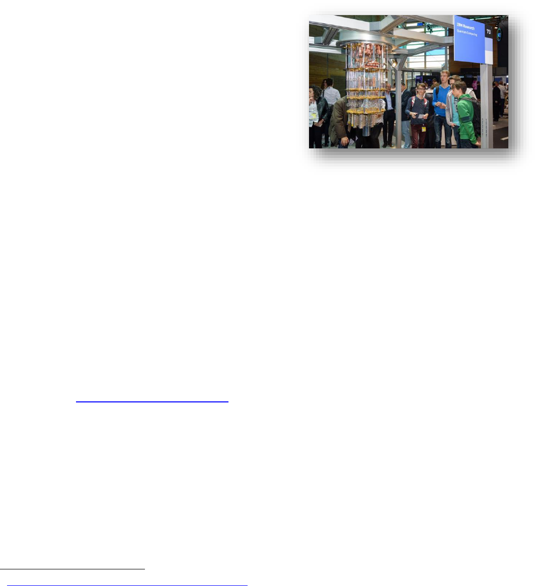
A Cryptographically Relevant Quantum Computer (CRQC) is a
computer that harnesses quantum mechanical phenomena as
computing elements and has operating parameters sufficient to break
some of today’s most commonly used cryptographic algorithms in a
short period of time. In some cases, the time to break a code is
expected to be measured in minutes or hours. Much smaller and less
able quantum computers exist today, but the creation of a CRQC is
beyond the ability of current technology. However, tens of billions of
dollars a year are being spent on research to achieve a CRQC. For
decades, the question was “can the issues and technological barriers
preventing the creation of a cryptography-breaking quantum
computer ever be overcome”. Now it is generally accepted that the
question is “when” will the issues be solved.
If you accept the premise that the arrival of a CRQC is a matter of “when”
and not “if”, your mindset should turn from one of simply monitoring progress to one of planning for the arrival. The
results of such planning will look different for each agency, organization, or company depending on the types of
assets they need to protect and the periods of time this protection must survive attacks by both conventional and
quantum means. That said, the planning processes for all entities have requirements in common. For example, they
each must determine their different classes of assets and what additional protections the assets will require to
withstand quantum attacks. Each class is defined by the length of time the assets must be protected, the value of
the assets, the exposure the assets have to quantum attack vectors (e.g., is your data normally transmitted over the
Internet) and the ability of currently used cryptography to protect the assets. Actions to protect each class of assets
must be defined; this includes creating plans, budgets, and times frames to implement the actions. Required
changes to current cryptography can range from increasing key lengths to replacement of some or all of the
cryptographic algorithms and methods in use. Regrettably, long-lived data that is currently protected with quantum-
vulnerable algorithms is already at risk, as attackers can capture the encrypted data and store it for future decryption
with a CRQC.
If you accept the inevitability of a CRQC, the central question is “when”. There is no consensus on this issue. You
will hear timeframes, from different experts, that vary wildly from 5 years to 30 years. A lot depends on the amount
of money spent on R&D and the ability to solve the remaining engineering problems. Another issue is we may not
know if or when the first CRQC is actually created, as some critical work is being conducted in secret. The best
predictions for the arrival of a CRQC typically assign a percentage denoting the level of confidence that a CRQC
will arrive by different future dates. Because of all the unknown variables, the event horizon for the arrival of a CRQC
covers a wide time period of at least 10 years. The period of time with the highest probability is between 10 and 20
years from now. As time passes, the confidence levels for the expected arrival times will most certainly become
greater, but that could mean less time to prepare.
The remainder of this document provides a much more detailed and technical review of quantum computers, their
development, how they threaten modern-day information security, and how to plan to mitigate the risks they pose
(including guidance on performing cryptographic transitions to quantum-safe algorithms). The ASC X9 Quantum
Computing Risk Study Group is composed of industry experts who will continue to track the issues and
development of a CRQC. Future editions of this report are planned as are other related reports. This group is open
to anybody that wishes to participate. Thank you for your interest.
ASC X9 IR-F01-2022
© ASC X9 Inc., 2022 – All Rights Reserved
2
2 Introduction
2.1 Background
This document provides a high-level, but broad, background on
quantum computing and the risks it is expected to pose to
cryptography—specifically, the cryptography used by the
financial services industry. Further, this document gives some
suggestions for organizations to assess and mitigate these
quantum risks.
The quantum computing landscape is undergoing an increasing
rate of change as more research and larger investment is
allocated to the development of quantum technologies. Across
the globe, more and more attention is being given to the
advancement of quantum computing, including fundamental
research, physical development, applications of the technology,
and so on. As the applications for quantum computing become
more varied and more practical, more people and organizations
are entering the field and contributing to its further development.
From Artificial Intelligence and Machine Learning (AI/ML) to applications in the Life Sciences and fundamental
scientific research, all the way to securing nation states from cyberattacks, the world is only now beginning to realize
the breadth of applicability for these next-paradigm machines.
According to a November 2021 report by International Data Corporation (IDC)
1
, the global market for quantum
computing is expected to increase to $8.6 billion (USD) by the end of 2027, up from $412 million in 2020. If this
estimate holds true, it represents a nearly 51% compound annual growth rate (CAGR) over a period of six years.
Further, the same IDC report forecasts that investment into quantum computing will increase with an 11.3% CAGR
over that same six-year period. This forecast also comes with the very reasonable suggestion that the projected
increase in investment can help to overcome current technological and engineering hurdles and propel the quantum
computing market into the next stages of maturity. Importantly, these estimates are very likely not to include
discretionary or secret government spending. And so, one can expect that the numbers presented in IDC’s
(unclassified) report fall short of the true numbers.
This document is the second edition of the X9 Quantum Computing Risks to the Financial Services Industry
Informative Report, with the first edition being published in late 2019. X9 is committed to tracking the ongoing
evolution in quantum computing and will continue to periodically revise this document. X9 also maintains a quantum
computing risk web page on its public web site that tracks major developments and has links to relevant documents
from other sites:
https://x9.org/quantum-computing/. Please contact X9 staff if you have information you would like
referenced on this page.
This document provides information tailored towards both management and technical people. The Overview section
(section 6) provides a shorter and less technical description of quantum computing, what it can and cannot do, and
the expected risks that it poses and how to mitigate them. While it is not possible to avoid all discussions of technical
issues, the Overview is written to be as non-technical as possible. The remaining sections of this document provide
a much more in-depth description and background of the software and hardware that make up a quantum computer.
This includes a discussion of the quantum algorithms that can crack certain cryptographic systems. This document
also discusses some of the hurdles that must still be overcome to create a large-scale, fault-tolerant, quantum
computer. Finally, the document gives recommendations for assessing and mitigating the quantum computing
threats, including steps that can be taken now to defend against future quantum-enabled attacks.
1
https://www.idc.com/getdoc.jsp?containerId=prUS48414121

ASC X9 IR-F01-2022
© ASC X9 Inc., 2022 – All Rights Reserved
3
As this report is primarily concerned with the nature of quantum computing and the risks quantum computing poses
to currently deployed cryptography, the potential non-cryptographic applications of quantum computing are not
detailed herein. By limiting the discussion to the information security impacts of quantum computing, it can be easy
for a reader to arrive at the erroneous conclusion that quantum computing will be a net-negative for society, and that
it will not have positive use-cases. In reality, there are numerous applications of quantum computing that are
expected to be enormously beneficial. Example applications include materials science, the design of
pharmaceuticals, chemical system simulations, artificial intelligence and machine learning, weather prediction, and
various other optimization problems (some of these examples are briefly discussed at the top of section 7). For a
sampling of positive applications of quantum computing within different industries (and other excellent information
on quantum computing), the reader is encouraged to download IBM’s The Quantum Decade report, which is freely-
available through the IBM website at the following URL:
https://www.ibm.com/thought-leadership/institute-business-
value/report/quantum-decade#.
2.2 Purpose
The purpose of this report is:
• To provide information on the threats and risks posed by large-scale, fault-tolerant, quantum computers,
including how quantum computers might be used to attack current cryptosystems, threat models for quantum-
enabled attacks, and other cryptographic and non-cryptographic considerations.
• To provide a description of how quantum computers operate, how they might be built, and to provide and
regularly update estimates for when a large-scale, fault-tolerant, quantum computer will be built.
• To provide a description of post quantum cryptography and the current state of post quantum algorithm
standardization.
• To provide suggestions for assessing and mitigating the threats and risks posed by quantum computing.
2.3 Scope
This report provides:
• A description of what quantum computing is, how it differs from classical computing, and the underlying
physical properties quantum computers use.
• A description of qubits, including an explanation of physical and logical qubits, possible ways to build
physical qubits, and ways to measure qubit quality.
• A description of the general technological and engineering requirements for building a large-scale, fault-
tolerant, quantum computer, and possible timelines for when one might be built.
• A description of different types of quantum computation devices.
• A description of post quantum cryptography and the ongoing efforts to standardize post quantum
cryptographic algorithms.
• A description of the quantum computing threat to current cryptosystems, protocols, and primitives.
• A description of the more general threats and risks posed by quantum computers, including threat models
and different components of the threats and risks.
• Suggestions for assessing and mitigating the threats and risks posed by quantum computers.
2.4 Future Editions and Participation
The ASC X9F Quantum Computing Risk Study Group (QCR SG) aims to regularly review and update the present
document. Participation in the development of future editions is open to X9 members and non-members alike. If
your organization is not an X9 member and wishes to participate in the Study Group, you are encouraged to contact
the Study Group Chair, Steve Stevens, at Steve.Steve[email protected] for more information about how you can contribute
your expertise to this important subject.

ASC X9 IR-F01-2022
© ASC X9 Inc., 2022 – All Rights Reserved
4
3 Normative References
Not applicable.
4 Terms and Definitions
For the purposes of this document, the following terms and
definitions apply:
4.1 Advanced encryption standard (AES)
AES is a symmetric encryption algorithm defined by FIPS PUB
197. With an appropriate mode of operation, it can provide
privacy (encryption) and integrity validation. AES uses an
internal block size of 128-bits, and allows keys of length 128-,
192-, and 256-bits.
4.2 Algorithm
A clearly specified mathematical process for computation; a set
of rules that, if followed, will give a prescribed result.
4.3 Asymmetric cryptography
Cryptography that uses two separate keys to exchange data, one to encrypt or digitally sign the data and one for
decrypting the data or verifying the digital signature. Also known as public key cryptography.
4.4 Bit string
An ordered sequence of zeros and ones (e.g., 0101011100).
4.5 Bit length
A positive integer that expresses the number of bits in a bit string.
4.6 Bloch Sphere
A three-dimensional geometric representation of the pure state space of a single quantum bit.
4.7 Block cipher
An invertible symmetric-key cryptographic algorithm that operates on fixed-length blocks of input using a secret
key and an unvarying transformation algorithm. The resulting output block is the same length as the input block.
4.8 Brute force attack
A trial-and-error method used to obtain information such as an encryption key, user password, or personal
identification number (PIN); the attacker simply tries all possible values of the key/password/PIN until he finds the
correct one. In a brute force attack, automated software is used to generate a large number of consecutive
guesses as to the value of the desired data.
4.9 Certificate
A set of data that uniquely identifies an entity, contains the entity’s public key and possibly other information, and
is digitally signed by a trusted party, thereby binding the public key to the entity identified in the certificate.
Additional information in the certificate could specify how the key is used and the validity period of the certificate.
NOTE: Also known as a digital certificate or a public key certificate.
4.10 Certificate Authority (CA)
A trusted entity that issues and revokes public key certificates.
ASC X9 IR-F01-2022
© ASC X9 Inc., 2022 – All Rights Reserved
5
4.11 Cipher
Series of transformations that converts plaintext to ciphertext using a cryptographic key.
4.12 Ciphertext
Data in its encrypted form.
4.13 Circuit
A way of expressing the sequence of operations required for implementing a given algorithm.
4.14 Circuit diagram
A graphical representation of a circuit.
4.15 Classical computer
A computer that operates using binary, Boolean, logic; can be modeled as a deterministic Turing Machine.
4.16 Code-based cryptography
The branch of post quantum cryptography concerned with the development of cryptographic systems based on the
difficulty of decoding error correcting codes.
4.17 Computer
A device that accepts digital data and manipulates the information based on a program or sequence of instructions
for how data is to be processed.
4.18 Confidentiality
Preserving authorized restrictions on information access and disclosure, including means for protecting personal
privacy and proprietary information.
4.19 Cryptanalysis
The study of mathematical techniques for attempting to defeat cryptographic techniques and information-system
security. This includes the process of looking for errors or weaknesses in the implementation of an algorithm or in
the algorithm itself.
4.20 Cryptography
Discipline that embodies principles, means and methods for the transformation of data to hide its information content,
prevent its undetected modification, and prevent its unauthorized use or a combination thereof.
4.21 Cryptographic agility
The capacity of a system to change the cryptographic algorithms or primitives it utilizes without requiring significant
changes to system infrastructure, and while minimizing disruption to system availability and functionality and that of
dependent systems.
NOTE: Also known as crypto agility.
4.22 Cryptographic hash function
A function that maps a bit string of arbitrary length to a fixed-length bit string. The function is usually expected to
have the properties of preimage resistance and collision resistance.
NOTE: A cryptographic hash function can satisfy additional security properties beyond those named above.
4.23 Cryptographic key
A parameter used in conjunction with a cryptographic algorithm that determines the specific operation of that
algorithm.
4.24 Discrete logarithm
Given any (discrete) group and elements of , an integer such that
is called the discrete logarithm
(of ) and is denoted by
.
ASC X9 IR-F01-2022
© ASC X9 Inc., 2022 – All Rights Reserved
6
4.25 Elliptic curve cryptography
The branch of cryptography concerned with the development of cryptographic systems based on the difficulty of
calculating discrete logarithms in elliptic curve groups.
4.26 Encryption
The process of using algorithmic schemes to transform plaintext information into a non-readable form called
ciphertext. A key (or algorithm) is required to decrypt the information and return it to its original plaintext format.
4.27 Ephemeral Key
Private or public key that is unique for each execution of a cryptographic scheme.
NOTE: An ephemeral private key is to be destroyed as soon as computational need for it is complete. An
ephemeral public key may or may not be certified.
4.28 Exhaustive key strength
If a cryptographic system employs a key with a bit length of , then there are
possible keys for a given instance
of that system. It takes at most
guesses to find the correct key via a brute force attack. In this case, the
exhaustive key strength of the system is bits.
4.29 Fault tolerance
The property that enables a system to continue operating properly in the event of the failure of one or more of its
components.
4.30 Grover’s algorithm
A quantum algorithm that finds, with high probability, the unique input to a black box function that produces a
particular output value. In theory, Grover's algorithm is known to reduce the security strength of symmetric
cryptosystems and primitives. However, due to real-world considerations (e.g., resource costs), Grover’s algorithm
might not be practical for cryptographic applications.
4.31 Integer
A member of the set of positive whole numbers , negative whole numbers , and zero .
4.32 Integer factor
A non-zero integer that can be divided evenly into another integer.
4.33 Integer factorization
The process of calculating the prime factors of a given integer. The Fundamental Theorem of Arithmetic states
that each positive integer has a unique factorization into prime numbers, excluding permutations of the ordering.
Negative integers also have unique prime factorizations up to ordering, but additionally include the non-prime
factor .
4.34 Intractable problem
A problem for which there is no known efficient algorithm (i.e., an algorithm with polynomial complexity) for solving
it. If such an algorithm is known, then the problem is said to be tractable.
4.35 Key agreement
A key-establishment procedure where the resultant keying material is a function of information contributed by two
or more participants, so that an entity cannot predetermine the resulting value of the keying material independently
of any other entity’s contribution.
4.36 Key establishment
A procedure that results in secret keying material that is shared among different parties.
ASC X9 IR-F01-2022
© ASC X9 Inc., 2022 – All Rights Reserved
7
4.37 Key management
The activities involved in the handling of cryptographic keys and other related parameters (e.g., IVs and domain
parameters) during the entire life cycle of the keys, including their generation, storage, establishment, entry and
output into cryptographic modules, use and destruction.
4.38 Lattice-based cryptography
The branch of post quantum cryptography concerned with the development of cryptographic systems based on the
difficulty of solving certain problems within discrete additive subsets of -dimensional euclidean space.
4.39 Logic gate
The mechanism used to perform logical operations on data. Examples of classical gates include the AND, OR,
and NOT gates. Examples of quantum gates include the Pauli X, Y, and Z gates, the Hadamard gate, and the
Phase-shift gate.
4.40 Logical qubit
A system composed of one or more physical qubits implemented to behave as a single qubit in a quantum circuit.
Quantum logic gates are applied to logical qubits during the execution of a quantum circuit.
4.41 Key pair
A public key and its corresponding private key; a key pair is used with a public-key algorithm.
4.42 Multivariate quadratic polynomial-based cryptography
The branch of post quantum cryptography concerned with the development of cryptographic systems based on the
difficulty of finding solutions to systems of multivariate quadratic polynomials.
4.43 Offline attack
Occurs when an adversary precomputes the relevant information to break the security of a system (such as a
cryptographic security protocol), with the intent to use that information sometime in the future when the system is
run.
4.44 Online attack
Occurs when an adversary attacks a system (such as a cryptographic security protocol) in real-time. For example,
while the system is in use or while the cryptographic protocol is actively being executed.
4.45 Physical qubit
A physical system that can exist in any superposition of two independent (distinguishable) quantum states and is
subject to noise and errors that may or may not be corrected for.
4.46 Plaintext
Intelligible data that has meaning and can be read or acted upon without the application of decryption. Also known
as cleartext.
4.47 Post quantum cryptography
The branch of cryptography concerned with the development of asymmetric cryptographic systems resistant to
attacks which utilize either quantum computers or classical computers.
NOTE: Post quantum cryptography is often used synonymously with quantum-safe cryptography (4.60). However,
the present document distinguishes the two terms.
4.48 Prime number
A positive integer not equal to 1 whose only integer factors are 1 and itself. For example, the first few prime
numbers are 2, 3, 5, 7, 11, 13, 17, 19, 23, and 29.
ASC X9 IR-F01-2022
© ASC X9 Inc., 2022 – All Rights Reserved
8
4.49 Private key
In an asymmetric (public) key cryptosystem, the key of an entity’s key pair that is known only by that entity.
NOTE: A private key may be used to compute the corresponding public key, to make a digital signature that may
be verified by the corresponding public key, to decrypt data encrypted by the corresponding public key; or together
with other information to compute a piece of common shared secret information.
4.50 Public key
That key of an entity’s key pair that may be publicly known in an asymmetric (public) key cryptosystem.
NOTE: A public key may be used to verify a digital signature that is signed by the corresponding private key, to
encrypt data that may be decrypted by the corresponding private key, or by other parties to compute shared
information.
4.51 Quantum advantage
A quantum-capable device is said to have quantum advantage (over classical devices) if it can perform useful
operations no classical device can.
4.52 Quantum annealing
A process for finding optimal, or near optimal, solutions to certain kinds of computational problems by finding low-
energy states of a quantum system that encodes the given computational problem.
4.53 Quantum bit (qubit)
A quantum-mechanical system, that can exist in two perfectly distinguishable states, that serves as the basic unit
of quantum information. Unlike classical systems, in which a bit exists in one state or the other, a qubit can exist in
a coherent superposition of both states simultaneously.
4.54 Quantum coherence
The property of a quantum system whereby it can maintain the purity of its state and not succumb to unintended
effects of the environment.
4.55 Quantum computer
A computer that operates and performs computations by leveraging the quantum mechanical properties of nature,
such as superposition, entanglement, and interference.
4.56 Quantum entanglement
Two or more quantum particles are entangled when their states cannot be described independently no matter their
physical separation; a measurement on one particle is correlated with information on the other(s).
4.57 Quantum error correction
The study of methods to protect quantum information from errors due to energy fluctuations, electromagnetic
interference, environmental disturbances, and other events which may have led to decoherence.
4.58 Quantum fidelity
A probabilistic measure of how similar a given quantum state is to a target quantum state.
4.59 Quantum measurement
The act, intentional or otherwise, of collapsing a quantum wave function. Quantum measurement can be thought
of as a transformation of a quantum superposition into a pure, classical state.
4.60 Quantum-safe cryptography
The branch of cryptography concerned with the development of cryptographic systems resistant to attacks which
utilize either quantum computers or classical computers. Unlike post quantum cryptography, which focuses only
on asymmetric systems, quantum-safe cryptography includes the study of asymmetric systems, symmetric
systems, and quantum key distribution.
ASC X9 IR-F01-2022
© ASC X9 Inc., 2022 – All Rights Reserved
9
4.61 Quantum superposition
The quantum mechanical property whereby a quantum system exists in two or more distinguishable quantum
states at the same time. Such a superposition of quantum states is itself a quantum state.
4.62 Quantum supremacy
The point where quantum computers can do things that classical computers can’t, regardless of whether those
tasks are useful.
NOTE: Today, this term is mostly used in a historical context. Quantum advantage is the more modern and
suitable metric.
4.63 Quantum threshold theorem
A theorem stating that if the rate of physical errors in a quantum circuit can be made low enough (below some
threshold), then the logical error rate can be made arbitrarily small by adding some number of additional quantum
gates.
4.64 Quantum volume
A metric for quantifying the largest random quantum circuit of equal width and depth that a given quantum
computer can successfully implement.
4.65 Shor’s algorithm
A quantum algorithm that can find the prime factors of a given input and calculate discrete logarithms. More
generally, Shor's algorithm is an efficient quantum algorithm for solving the Hidden Subgroup Problem. Shor’s
algorithm breaks classical asymmetric cryptosystems such as RSA and those based on Elliptic Curve
Cryptography.
4.66 Static key
Private or public key that is common to many executions of a cryptographic scheme.
NOTE: A static public key may be certified.
4.67 Stream Cipher
A symmetric encryption method in which a cryptographic key and algorithm are applied to each binary digit in a
data stream, one bit at a time.
4.68 Supersingular isogeny-based cryptography
The branch of post quantum cryptography concerned with the development of cryptographic systems based on the
difficulty of computing isogenies between supersingular elliptic curves.
4.69 Symmetric cryptography
Cryptography that uses the same secret key for its operation and, if applicable, for reversing the effects of the
operation (e.g., an AES key for encryption and decryption).
NOTE: The key shall be kept secret between the two communicating parties.
4.70 Symmetric key
A cryptographic key that is used to perform both the cryptographic operation and its inverse (e.g., to encrypt, decrypt,
create a message authentication code, or verify a message authentication code).
4.71 Unitary matrix
A square, complex-valued, matrix with inverse equal to its conjugate transpose.
ASC X9 IR-F01-2022
© ASC X9 Inc., 2022 – All Rights Reserved
10
5 Symbols and Abbreviations
For the purposes of this document, the following symbols and abbreviated terms apply:
5.1 3DES
Triple Data Encryption Algorithm
NOTE: Also known as the Triple Data Encryption Algorithm (TDEA) and Triple Data Encryption Standard (TDES)
5.2 AAD
Additional Authenticated Data
5.3 ABE
Attribute-based Encryption
5.4 AEAD
Authenticated Encryption with Associated Data
5.5 AES
Advanced Encryption Standard
5.6 AH
Authentication Header
5.7 AI
Artificial Intelligence
5.8 BC
Business Continuity
5.9 BIA
Business Impact Assessment
5.10 BIKE
Bit-flipping Key Exchange
5.11 BSI
Federal Office for Information Security
NOTE: BSI is an agency of the German government. The above is an English translation of the German name:
Bundesamt für Sicherheit in der Informationstechnik.
5.12 CBC
Cipher Block Chaining
5.13 CCCS
Canadian Centre for Cybersecurity
5.14 CFDIR
Canadian Forum for Digital Infrastructure Resilience
5.15 CSA
Cloud Security Alliance
5.16 COW
Coherent One-Way
ASC X9 IR-F01-2022
© ASC X9 Inc., 2022 – All Rights Reserved
11
5.17 CRYSTALS
Cryptographic Suite for Algebraic Lattices
5.18 CRQC
Cryptographically Relevant Quantum Computer
5.19 CSPRNG
Cryptographically Secure Pseudorandom Number Generator
5.20 CSS
Calderbank-Shor-Steane
5.21 DES
Data Encryption Standard
NOTE: Also known as the Data Encryption Algorithm (DEA).
5.22 DH
Diffie-Hellman
5.23 DHE
Ephemeral Diffie-Hellman
5.24 DR
Disaster Recovery
5.25 DSA
Digital Signature Algorithm
5.26 DTLS
Datagram Transport Layer Security
5.27 ECC
Elliptic Curve Cryptography
5.28 ECDH
Elliptic Curve Diffie-Hellman
5.29 ECDSA
Elliptic Curve Digital Signature Algorithm
5.30 ENISA
European Union Agency for Cybersecurity
NOTE: The abbreviation comes from the original name of the agency: the European Network and Information
Security Agency.
5.31 ESP
Encapsulating Security Payload
5.32 ETSI
European Telecommunications Standards Institute
5.33 FALCON
Fast-Fourier Lattice-based Compact Signatures over NTRU
ASC X9 IR-F01-2022
© ASC X9 Inc., 2022 – All Rights Reserved
12
5.34 FASP
Fast and Secure Protocol
5.35 FHE
Fully Homomorphic Encryption
5.36 FIM
Federated Identity Management
5.37 FIPS
Federal Information Processing Standard
5.38 FT
Fourier Transform
5.39 FTPS
File Transfer Protocol Secure
NOTE: FTPS is distinct from SFTP.
5.40 GCHQ
Government Communications Headquarters
5.41 GDPR
General Data Protection Regulation
5.42 GeMSS
Great Multivariate Short Signature
5.43 HMAC
Hash-based Message Authentication Code
5.44 HQC
Hamming Quasi-Cyclic
5.45 HRNG
Hardware Random Number Generator
5.46 HSP
Hidden Subgroup Problem
5.47 HTTPS
Secure Hypertext Transport Protocol
5.48 IANA
Internet Assigned Numbers Authority
5.49 IBM
International Business Machines
5.50 ICV
Integrity Check Value
5.51 IETF
Internet Engineering Task Force
ASC X9 IR-F01-2022
© ASC X9 Inc., 2022 – All Rights Reserved
13
5.52 IID
Independent and Identically Distributed
5.53 IIoT
Industrial Internet of Things
5.54 IKEv2
Internet Key Exchange version 2
5.55 IoT
Internet of Things
5.56 IPSec
Internet Protocol Security
5.57 ISO
International Organization for Standardization
NOTE: ISO is not technically an abbreviation. Rather, ISO is a convenient short form for the organization’s name,
selected to avoid the issue of the abbreviation being different in different languages.
5.58 ISP
Internet Service Provider
5.59 IV
Initialization Vector
5.60 KDF
Key Derivation Function
5.61 KEM
Key Encapsulation Mechanism
5.62 LMS
Leighton-Micali Signature
5.63 MIT
Massachusetts Institute of Technology
5.64 ML
Machine Learning
5.65 NISQ
Noisy Intermediate-Scale Quantum
5.66 NIST
National Institute of Standards and Technology
5.67 NSA
National Security Agency
5.68 NTRU
Number Theorists R Us
5.69 PAN
Primary Account Number
ASC X9 IR-F01-2022
© ASC X9 Inc., 2022 – All Rights Reserved
14
5.70 PHI
Protected Health Information
5.71 PIC
Photonic Integrated Circuit
5.72 PII
Personally Identifiable Information
5.73 PKI
Public Key Infrastructure
5.74 PQC
Post Quantum Cryptography
5.75 PRF
Pseudorandom Function
5.76 PRNG
Pseudorandom Number Generator
NOTE: Also known as a Deterministic Random Bit Generator (DRBG).
5.77 QAOA
Quantum Approximate Optimization Algorithm
5.78 QEC
Quantum Error Correction
5.79 QFT
Quantum Fourier Transform
5.80 QKD
Quantum Key Distribution
5.81 QRNG
Quantum Random Number Generator
5.82 RNG
Random Number Generator
5.83 SIKE
Supersingular Isogeny Key Encapsulation
5.84 RSA
Rivest-Shamir-Adleman
5.85 SCADA
Supervisory Control And Data Acquisition
5.86 SCP
Secure Copy
ASC X9 IR-F01-2022
© ASC X9 Inc., 2022 – All Rights Reserved
15
5.87 SFTP
Secure File Transfer Protocol
NOTE: SFTP is distinct from FTPS.
5.88 SHA
Secure Hash Algorithm
5.89 SIKE
Supersingular Isogeny Key Exchange
5.90 SLA
Service Level Agreement
5.91 SNDL
Store-Now, Decrypt-Later
NOTE: Also known as Harvest-Now, Decrypt-Later (HNDL)
5.92 SPHINCS+
Stateless Practical Hash-based Incredibly Nice Cryptographic Signatures Plus
5.93 SSH
Secure Shell
5.94 SSL
Secure Sockets Layer
5.95 SSO
Single Sign On
5.96 TLS
Transport Layer Security
5.97 TRNG
True Random Number Generator
5.98 URL
Uniform Resource Locator
5.99 VPN
Virtual Private Network
5.100 VQE
Variational Quantum Eigensolver
5.101 WEF
World Economic Forum
5.102 XMSS
eXtended Merkle Signature Scheme
5.103 Y2Q
Years to Quantum
Note: The term is also used to describe the year in which the first CRQC is built.

ASC X9 IR-F01-2022
© ASC X9 Inc., 2022 – All Rights Reserved
16
6 Overview of Quantum Computing Risks, Timelines, and Mitigations
6.1 Quantum Computing vs Classical Computing
The computers we know and use today are also known as
classical computers. These machines work by taking in some
input, and then by using something called an instruction set,
they manipulate that input using a classical, Boolean logic (i.e.,
using the logical operations AND, OR, and NOT), to get some
desired output. The inputs, when reduced to their most basic
level, are simply strings of bits (i.e., 0's and 1's), which basically
indicate "on" or "off", or "yes" or "no". By using these basic
binary inputs, together with some clever instruction set,
classical computers can do the operations necessary to
perform computations. In practice, classical computers are
restricted by resource requirements such as time, memory, and
computational power. Even so, today's classical computers are
marvels of scientific achievement. The smartphone in your
pocket has more computing power and memory than was used by Apollo 11's Guidance Computer when humankind
was first put on the Moon in 1969. And not just a little bit more power and memory, modern smartphones have more
than a million times the memory of the Apollo 11 Guidance Computer, and around one hundred thousand times the
computing power. Never mind what today's supercomputers are capable of.
Classical computers have come a long way, but they still have their limits in terms of solving many practical
computational problems. In theory, given unbounded resources to use (including as much time as is necessary), a
classical computer can solve any computational problem that can be solved. In reality, there are not unbounded
resources available for any classical machine, including large high-performance computing clusters. As a result,
certain computational problems that we would like to solve remain out of reach.
Quantum computers, first theorized by the theoretical physicist Richard Feynman in 1982, are devices that operate
not only on classical logic, but rather on an extended quantum logic that harnesses the physical properties of nature,
the properties of quantum mechanics. The fundamental unit of classical computation is the (classical) bit, and the
fundamental unit of quantum computation is the quantum bit, or more commonly, the qubit.
Suppose for example that you flipped a coin. You know that when the coin lands, it will come up either heads or tails
(ignoring double-sided coins and the possibility of the coin landing on its edge). But what is the value of the coin
before it lands? At any point in time while the coin is in the air, is it heads? Tails? Neither? Both? There is not really
a good answer to this question, and without a complete understanding of the prior state of the coin and the forces
imparted on it the end-value is unknowable until the coin lands. Thus, we assign a probability to each outcome: a
50% chance of heads and 50% chance of tails.
When you measure a qubit (i.e., after the coin lands), its state will be either (tails) or (heads), which you can
easily read off. However, prior to measurement, the state of the qubit is actually a combination of and . This
combination of values is called a superposition and is essentially what is meant in popular science articles that
describe quantum computing by saying things like “a qubit takes on all possible values at the same time”, or “a qubit
is every possible value in-between and , at the same time”. An unmeasured qubit can indeed be in a state that
is simultaneously both of those values, but just not necessarily in equal parts. The sizes of the parts are weighted
according to certain “quantum probabilities” called probability amplitudes.
To be clear, the qubit does not have some “true” value of or that you are just unaware of until you measure it.
The qubit’s state is a simultaneous combination of values (which is itself a distinct state) and becomes either or
only after the qubit is measured. The catch is that when the qubit is measured, it does not necessarily return a or
a with equal probability. The probability of measuring either or is governed by how close the qubit state was to
either or when it was measured. This can be explained mathematically with linear algebra (section 7.2). The art
of quantum computing is about manipulating and influencing qubits (and the probability amplitudes of all the possible
ASC X9 IR-F01-2022
© ASC X9 Inc., 2022 – All Rights Reserved
17
outcomes) so that when they are measured, they return (with high probability) the correct answers to the
computational problems being asked.
To summarize so far, in classical computing, a bit always has a concrete and knowable value of or , and never a
combination of the two. In quantum computing, a qubit can have an undetermined value, or state, this is some
combination of and . But computations with single qubits are not particularly interesting. Similar to classical
computation, the real power of quantum computation lies in what happens when we add more and more qubits.
A binary string with length has
possible values. We say that the number of values is exponential in the length
of the string. For example, a length-2 string has
possible values, namely . Because classical
computers operate on concrete values, a classical computer can only operate on one of these four values at a time.
With quantum computers, two qubits can be in a state that is some combination of , but only one of
these values will be returned when the qubits are measured. That is, two qubits, prior to being measured, can be in
a state that is a combination of each possible value a length- binary integer can be.
Generalizing this, qubits can be in a state that is some combination of the
possible values a length- binary
integer can be. By performing quantum logic operations on such a state, it is possible to compute certain properties
of certain mathematical functions of all those values. By computing the function once on all those input values
simultaneously, the result is a state that is a quantum superposition of all the function output values. This is often
referred to as quantum parallelism. By contrast, a classical computer would need to compute that function on each
value separately, which would require an exponential number of resources to do (i.e., time or memory/storage
space).
To further illustrate quantum parallelism, a two-qubit quantum computer can in some sense operate on all four of
the possible values a length-2 binary integer can take on. By adding a third qubit, the machine can operate on
values concurrently. With each additional qubit, the number of states that can be simultaneously operated on is
doubled. To double the number of states to simultaneously operate on in a classical computer, you would need to
essentially double the size of the computer. If you doubled the size of a classical computer 100 times you would
have a computer larger than the planet, whereas adding 100 qubits to a quantum computer results in a comparatively
insignificant overall size increase.
It is important to clarify a common misunderstanding of quantum computing. Quantum parallelism does not allow a
quantum computer to inspect or try out exponentially many solutions to a computational problem in parallel. A
quantum computer is severely limited in the kinds of ways it can produce meaningful output from operating on
superpositions of function-values for a particular computational problem.
There are certain computational problems that are just simply beyond the capabilities of any classical machine, or
cluster of machines, to solve; particularly when the input sizes get larger and larger. These problems are said to be
intractable on classic machines and are usually referred to as (classically) hard problems. Some of these classically
hard problems will not be beyond the capabilities of quantum computers to solve. They are tractable on quantum
computers (of sufficient size). In general, this is a wonderful thing, and it opens many new areas of scientific
achievement and discovery. Unfortunately, some of these classically hard problems that are solvable by quantum
computers are precisely the hard problems that underly the security of today’s widely deployed cryptographic
algorithms, primitives, and protocols.

ASC X9 IR-F01-2022
© ASC X9 Inc., 2022 – All Rights Reserved
18
6.2 Quantum Computing Risks to Cryptography
There are two main quantum algorithms that impact the security
of today’s cryptographic algorithms and primitives: Grover’s
Algorithm and Shor’s Algorithm. Grover’s Algorithm impacts the
security of symmetric key systems such as AES and primitives
such as hash functions. Shor’s Algorithm impacts the security
of asymmetric (public key) systems such as RSA and elliptic
curve-based systems. Moreover, security protocols that employ
quantum-vulnerable systems and primitives themselves
become vulnerable to quantum-enabled attacks. The following
gives a high-level description of how these two quantum
algorithms threaten today’s widely deployed cryptographic
algorithms, primitives, and protocols.
Grover’s Algorithm is a quantum algorithm for solving the
Unstructured Search Problem (section 8.1.3), which is
commonly analogized as the problem of searching for a needle
in a haystack. Grover’s Algorithm is often said to reduce the security of symmetric key schemes and primitives by
half; that is, what had bits of security against classical attacks now has bits of security against quantum-
enabled attacks
2
. If true, symmetric key lengths and hash function output lengths would need to be doubled to
maintain the same level of security. While this discussion of Grover’s Algorithm is sufficient for popular articles, it is
not exactly correct in practice. In fact, by making modest assumptions about the time it takes to perform each
operation, and limits on the length of time the attacker has to attack, it has been shown that only a fixed number of
extra bits is required to maintain security, where that number depends on the symmetric system or primitive under
consideration. Therefore, Grover’s Algorithm reduces the security of symmetric-based systems and primitives, but
it does not cut the security in half. NIST in their Post-Quantum Cryptography FAQ states “it is quite likely that Grover’s
algorithm will provide little or no advantage in attacking AES, and AES 128 will remain secure for decades to come
3
."
Regardless, risk-averse organizations can still move to key lengths of 192 or 256 bits.
Shor’s Algorithm is an efficient quantum algorithm that can be used to both calculate the prime factors of large
integers and calculate discrete logarithms. The difficulty of factoring large integers is the basis for the security of the
RSA algorithms (which are used for encryption, digital signatures, and key establishment), and the difficulty of
calculating discrete logarithms is the security basis for elliptic curve cryptography (ECC, which is used for digital
signatures and key establishment). It is possible that large-scale quantum computers will be able to solve these hard
problems using Shor’s Algorithm in a matter of hours, and possibly in only a matter of minutes once the technology
sufficiently evolves.
With Grover’s Algorithm, the security of symmetric key systems and hash functions is reduced, but the security loss
can be overcome with an increase in key and output lengths. In the case of Shor’s Algorithm, increasing asymmetric
key lengths is not an effective remedy. In fact, if asymmetric key lengths were doubled, say from bits to qubits,
it would take the addition of only logical qubits (section 7.3.2) for the quantum computer to be able to break the
schemes just as effectively as before
4
. As RSA keys are usually only a few thousand bits long and ECC keys only
a few hundred, it is not difficult to see that doubling an asymmetric key length is not an effective defense against a
scalable quantum computer. Moreover, asymmetric systems tend to be slower and more resource intensive than
symmetric systems. Therefore, the performance hit one would take from doubling asymmetric key lengths would
almost certainly not be worth the small increase in security; assuming the system can accommodate the larger keys
2
Note that Grover’s Algorithm cannot inspect or try out all the “pieces of hay” of the “haystack” simultaneously. This is an example
of how quantum parallelism does not give quantum computers “fully exponential” computing power.
3
https://csrc.nist.gov/Projects/post-quantum-cryptography/faqs
4
In practice, more than new qubits may be required depending on the qubit architecture, error correction methods, algorithm
requirements, and other factors.

ASC X9 IR-F01-2022
© ASC X9 Inc., 2022 – All Rights Reserved
19
in the first place. RSA and elliptic curve-based algorithms are the most widely used public key algorithms today, and
a break in either of them represents an unprecedented risk to today’s information security systems.
Given their susceptibility to quantum-enabled attacks, it is recommended that organizations wholly transition away
from RSA and elliptic curve-based systems and adopt algorithms resistant to quantum-enabled attacks (such
algorithms are known as post quantum algorithms). In early July 2022, the National Institute of Standards and
Technology (NIST) announced that it had selected several post quantum algorithms for standardization. NIST
expects to finalize the standards for the selected algorithms around 2024. Once standardized, it is recommended
that organizations use NIST-approved post quantum algorithms instead of RSA and elliptic curve-based systems.
Importantly, organizations do not have to wait until NIST completes their standardization process to begin planning
a migration to post quantum cryptography. This is discussed further in section 6.5, and more completely in section
13.
Finally, cryptographic algorithms are at the core of information security. Hence, any system that uses quantum-
vulnerable cryptography becomes vulnerable to quantum-enabled attack. This includes critically important security
protocols such as TLS, SSH, and the different VPN technologies, to only name a few. Some protocols are possibly
more resistant to quantum-enabled attacks than others (e.g., if attacks against them need to be carried out in real-
time vs situations where precomputation can be used). However, the general recommendation is that all quantum-
vulnerable security protocols also be updated to use post quantum cryptography when the NIST standards are
completed.
6.3 Other Quantum Computing Risks
The threats posed by large-scale quantum computers are not
limited to cryptography. If the cryptography employed by an
organization is successfully attacked, then all sorts of operational,
reputational, and legal issues can follow. These considerations are
not new and are not necessarily unique to quantum computing.
However, given the susceptibility of currently deployed
cryptography to quantum computing attacks, these non-
cryptographic threats become especially concerning and require
careful consideration to mitigate.
The precise risks and vulnerabilities vary from organization to
organization, and there is no cookie-cutter solution suitable for
everyone. To properly mitigate quantum-risk, each organization
needs to assess and understand its own situation. The following gives a high-level description of various risks that
an organization might face in the presence of large-scale quantum computers. As a general statement, organizations
are encouraged to incorporate quantum-enabled attacks into their Business Impact Assessments (BIAs), and in their
Business Continuity (BC) and Disaster Recovery (DR) planning.
Many organizations have legal or contractual obligations to protect the confidentiality of certain data for certain
lengths of time. Long-term confidentiality requirements are threatened by Harvest-and-Decrypt attacks
5
, whereby
an attacker captures encrypted data in transit, stores that data, and decrypts it when they gain access to a sufficiently
capable quantum computer. This means that data whose confidentiality is required far into the future might very well
be at risk today, as it has already been captured (in its encrypted form) by some adversarial entity. In fact, it is
believed that various nation-state actors have been harvesting large amounts of encrypted data for some time, for
precisely this reason. An important question an organization should ask itself is “where and how might an attacker
capture my encrypted data?”. For example, an attacker might broadly harvest data at industry events (e.g.,
conferences or workshops) or at particular locations (e.g., hotels or airports). They might also tailor their attacks to
specific individuals, whether at the office, at home, or somewhere else. In possibly the most devastating scenario,
an attacker can gain access to encrypted storage media (e.g., through improper disposal or data sanitization). All of
5
Also known as "Harvest-Now, Decrypt-Later”, “Store-Now, Decrypt-Later” (SNDL), and by other similar variations.
ASC X9 IR-F01-2022
© ASC X9 Inc., 2022 – All Rights Reserved
20
this raises critical questions about how to remain compliant with privacy regulations or other legal obligations
(including contractual obligations) in a situation where large-scale quantum computers can successfully break
today’s cryptography.
Another issue is that of long-term identities and fraudulent authentication. For a variety of reasons, many systems
are difficult, if not impossible, to upgrade. Maybe there are technological constraints on the system, maybe they are
physically difficult to access, or maybe availability or interoperability requirements prevent significant changes to the
system. Regardless, if a system employs long-lived identities, then it might be possible for a quantum-capable
attacker to recover the private keys of those identities, or otherwise break the authentication mechanisms. If an
attacker can gain access to a system, they can cause significant harm and damage. For example, they can create
malicious code-updates and sign them with the authentic private key. This means that reliant systems will accept
the updates as authentic and install them accordingly. If a system is part of critical infrastructure and an attacker
gains access, then human safety can be put at significant risk. Examples here include SCADA systems or Industrial
IoT devices. An attacker might also be able to use authentic credentials to issue yet more credentials to other
attackers. In this case, an attacker acts as a gateway for other attackers to gain access to the system. The loss of
system or data availability due to quantum-enabled attacks might require the organization to enact its BC or DR
procedures, and if the issues are not remediated in a timely fashion, the cost to the organization can be
insurmountable (e.g., due to operational disruption or reputational harm). Another attack against long-term identities
is impersonating legitimate users. Perhaps a user has long-lived credentials for a banking system, or a distributed
ledger or blockchain application. If an attacker gains access to the private credentials of that user, they might be
able to launch devastating financial attacks. For example, redirecting funds, engaging in other financial transactions,
or entering obligations on the behalf of the legitimate user.
Long-term data integrity can also be put at risk by quantum-enabled attackers. Attackers might be able to forge or
otherwise alter important ownership documents such as land records or property deeds. Digitally owned assets,
such as Non-Fungible Tokens (NFTs) can also be at risk here, depending on how the assets are cryptographically
protected. Registered trademarks, patents, and patent applications might also have their ownership called into
question if a quantum-enabled attacker can produce authentic-looking documents claiming alternative ownership.
Long-term contracts are at risk of being digitally altered and having their terms manipulated; the same concern might
also apply to shorter-term contracts as well, such as Service Level Agreements (SLAs). Other examples of at-risk
documents include mortgage documents, documents relating to loans (e.g., automotive or lines of credit), documents
relating to securities lending, or subpoenas. It is possible that the concerns presented here can be mitigated by
providing original paper copies of the at-risk documents. However, not all (legal) documents have paper copies, and
not all paper copies are easy to locate and produce. Even if an original paper copy can be provided, significant harm
can be done by the time it is produced and authenticated.
In a similar vein as the above, digital evidence is at risk of future manipulation due to quantum computing attacks.
Again, these attacks can occur if an attacker is able to recover the private keys, or other credentials, of a legitimate
entity. Examples here include the manipulation of audit logs, including financial audit records, legal audit records, or
network logs and other reports. Digital communications face a similar risk, such as e-mail or text message
exchanges. Just as with the manipulation of contracts, manipulation of digital communications can make it seem as
though a party said things, or made commitments, which they did not. This is particularly concerning in the context
of evidence such as written testimony in digital format, and video, audio, or photographic evidence.
Digital data in general is put at risk of manipulation and counterfeiting. For example, an attacker might be able to
create or modify incriminating documents to make it look as though some other entity engaged in illegal or unethical
behavior. Finally, legally protected personally identifiable information (PII) and protected health information (PHI)
are put at the same risk of manipulation, counterfeiting, and disclosure. Besides legal requirements to protect such
data, and the possible legal ramifications of failing to do so, human safety and well-being is threatened by attacks
against such personal data. It is therefore paramount that personal information (financial, health, legal, etc.) be
adequately protected in a post quantum age, and that serious consideration for how to do so is given well before
the advent of quantum computers powerful enough to threaten today’s cryptosystems.

ASC X9 IR-F01-2022
© ASC X9 Inc., 2022 – All Rights Reserved
21
6.4 Expected Timelines for Quantum Computers
For organizations looking to fortify against quantum-attacks, the
question of “when will there be a quantum computer capable of
threatening our security?” is a critical one to ask. To plan an
effective quantum-risk migration strategy, the organization needs
to have some idea of the timelines involved. Unfortunately,
predicting exactly when a security-threatening quantum computer
will appear is tremendously difficult. There are numerous factors
that can affect the rate at which quantum computers develop,
including technological, economic, societal, and political factors
(see Table 5 in section 7.10 for specific examples of such factors).
To compound the difficulty, the effect of each factor is not
necessarily independent of the others; it is possible that an
advance in one area can lead to a cascade of advances in other
areas.
Therefore, to obtain a reasonable estimate of when a large-scale, fault-tolerant, quantum computer will arrive
requires keeping current with the different factors that can affect the arrival timeline. Doing so will also allow
organizations to revise their estimates as time progresses. However, for many organizations, tracking all the different
factors can be overly burdensome. Thankfully, organizations do not need to come up with estimates entirely on their
own. While it will be important for organizations to keep up to date with the state of the art—as well as they can—to
better inform their own migration plans (section 13), organizations can also benefit from the timeline estimates of
leading researchers and quantum computing experts. Some such estimates are discussed below.
A survey of subject matter experts was conducted in 2021 and published by the Global Risk Institute
6
. The results
of the survey include estimates of the likelihoods during different intervals over the next 30 years of a quantum
computer being able to break RSA-2048 within 24 hours. For example, 10 of the 46 respondents gave a likelihood
estimate of 30% or higher during the next 5 years, but 46 out of 46 respondents gave an estimate of 30% or higher
over the next 30 years (from the time of the survey). 15 respondents estimated a 50% or greater likelihood over the
next 10 years, and 28 respondents said 50% or greater over the next 15 years. The likelihoods reported for each
question asked in the survey are rather granular, and the reader is encouraged to review that report.
Another estimate has been put forth by the Cloud Security Alliance (CSA), referred to as the Countdown to Y2Q
(Years to Quantum, or the year when cryptography-breaking quantum computers first arrive)
7
. The CSA’s estimate
is inherently different from other expert estimates in that 1) it proposes a specific time and date for the arrival of a
cryptography-breaking quantum computer (namely, April 14, 2030), and 2) it is intended to be more of a motivation
for quantum-readiness than a high-confidence prediction. Per the Global Risk Institute’s report discussed above, an
estimate of 2030 is not unreasonable, but it is arguably a risk-averse estimate. Again, the Global Risk Institute’s
report specifically asked about a quantum computer capable of breaking RSA-2048 within 24 hours. The CSA’s
estimate is less specified. Quoting from the CSA website, “[o]n April 14, 2030 CSA estimates that a quantum
computer will be able to break present-day cybersecurity infrastructure.” And so, the reader should be careful about
directly comparing the different estimates. However, as mentioned above, the CSA estimate is largely intended to
act as an incentive for organizations to begin planning their quantum-safe migrations. By selecting a concrete date
in the relatively near future it is believed that organizations will be better motivated to become quantum-safe sooner
rather than later. For more details, the reader can watch the recorded presentation from the CSA Research Summit
8
.
The estimate for the arrival of a cryptography-breaking quantum computer is only one of the timeline variables
required for planning and executing a quantum-safe migration strategy. Two other useful variables are the length of
6
Quantum Threat Timeline Report 2021 https://globalriskinstitute.org/publications/2021-quantum-threat-timeline-report/
7
CSA’s Countdown to Y2Q https://cloudsecurityalliance.org/research/topics/quantum-safe-security/
8
Cloud Security in the Quantum Era: Getting Ready for Y2Q https://www.brighttalk.com/webcast/16947/534758
ASC X9 IR-F01-2022
© ASC X9 Inc., 2022 – All Rights Reserved
22
time the organization’s assets need to be protected for and the length of time required to implement quantum-safe
protections for those assets. These variables are often presented in the context of Mosca’s XYZ Theorem, due to
Michele Mosca. The three variables are usually referred to as the X, Y, and Z variables, and they are described
below.
X) Shelf-life: the number of years the asset must be protected.
Y) Migration-time: the number of years needed to migrate the asset to a quantum-safe state.
Z) Threat-time: the number of years before threat actors can access Cryptographically Relevant Quantum
Computers (section 7).
If the threat-time is shorter than the sum of the shelf-life time and the migration-time, the organization may not be
able to protect their assets against quantum attacks for the required number of years. That is, if Z < X + Y, then
threat actors can access CRQCs during a time when the assets still require protection, but before that protection
uses quantum-safe cryptographic algorithms. Conversely, if Z > X + Y, then the organization should be able to
protect their assets against quantum attacks before quantum attacks are feasible.
It is important to understand that the values of X, Y, and Z can be different for different assets. X can be different
because one type of asset may have a different lifetime from another one. Y can be different because an organization
is likely to implement quantum-safe cryptographic protections in phases, and one type of asset may start using
quantum-safe algorithms before another one. Z can be different because some assets can be protected using
different conventional algorithms (e.g., RSA vs. Elliptic Curve Cryptography) or different key lengths than other
assets. The scale of quantum computer needed to attack one algorithm or key length can be different from what is
required to attack another one.
The result of these variabilities is that Mosca’s XYZ Theorem should be applied separately for each class of data
assets. Each will have its own values for X, Y, and Z. The worst case among these determines when your entire
system will be safe against quantum attacks. Furthermore, you should always be very conservative in your
determination of the X, Y, and Z values. People tend to make estimates that are overly optimistic, but it is critically
important to have your assets protected with quantum-safe algorithms before any attack with a CRQC is possible.
Therefore, you should tend toward overestimating the values of X and Y, and underestimating the value of Z.
Note that a portion of the migration timeline Y will depend on assets such as hardware and software that implement
cryptographic algorithms used by your applications. When calculating the value of Y, you should consider the time
it will take to replace that hardware and software with suitable quantum-safe alternatives, and to integrate those into
your system.
Section 12 and section 13 of the present document discuss how to use Mosca’s XYZ Theorem in the creation of a
quantum-safe migration strategy and roadmap, but a summary of that discussion is included in section 6.5 below.
The Quantum Threat Timeline Report discussed in section 7.10 is primarily concerned with estimating the Z variable.

ASC X9 IR-F01-2022
© ASC X9 Inc., 2022 – All Rights Reserved
23
6.5 Assessing and Mitigating Risks
Before an organization can mitigate its quantum-risks, it must be
able to identify where it is vulnerable, understand why those
vulnerabilities exist, and be familiar with the available solutions.
Moreover, to budget for and select the most appropriate solutions,
the organization needs to have some reasonable estimate of how
much damage can be caused by exploit of those quantum-
vulnerabilities. This suggests that there will be different steps of the
organization’s quantum-safe migration. These different steps can
be described in a quantum-safe migration strategy, and they can
be achieved according to the timelines in an associated roadmap.
Section 13 spells out the differences between mitigation and
migration, and a strategy vs a roadmap, but the important take-
away is that a migration takes the organization from a quantum-
vulnerable state to a quantum-safe state, and a roadmap is a tool
for putting the migration strategy into action (e.g., through timelines, milestones, and a logical ordering of the steps
of the migration strategy). After the migration, ongoing quantum-risk mitigation will likely be subsumed into the
organization’s general cyber-risk management program.
The following discusses a high-level quantum-safe migration strategy that organizations can use as a guide for their
own quantum-safe migrations. This same strategy is discussed in significantly more detail in section 13. The present
document is designed to provide enough information for a reader to be able to make substantial progress on each
of the steps in the strategy. Moreover, there are other publicly available guides, frameworks, and reports to help
organizations understand the quantum risks to information security and to plan quantum-safe migrations; several
such works are listed in Table 9 in section 13. As there are no one-size-fits-all migration strategies, organizations
are encouraged to study multiple strategies and techniques for mitigating quantum-risk, and formulate their own
plans based on their own specific needs.
1) Gain a general understanding of quantum computing and its impacts to information security.
2) Gain a general understanding of the tools, techniques, and standards that can be used to protect against
quantum-enabled attacks and stay up to date with the development of new tools, techniques, and standards.
3) Understand where and how the organization currently consumes quantum-vulnerable cryptography (including
the organization’s use of quantum-vulnerable standards) and identify the non-cryptographic vulnerabilities as
well (such as those described in section 12.2). This step should also include identifying the cryptographic and
non-cryptographic vulnerabilities throughout the organization’s supply chains.
4) Map the items identified in 2) to the vulnerabilities identified in 3). That is, identify and select the appropriate
quantum-safe controls for the cryptographic and non-cryptographic vulnerabilities of the organization.
Additionally, the organization should engage their suppliers to learn what their plans are towards
implementing their own quantum-safe migration strategies.
5) Engage in proof-of-concept (or similar) activities to validate that the controls identified in 4) are appropriate
for the organization.
6) Create a plan to acquire and implement the controls validated in 5).
Table 1: An example quantum-safe migration strategy
Step 1) Understand quantum computing and its impacts
Gaining knowledge and awareness of the quantum computing impact to information security is a natural first step in
any migration strategy; a summary of this information was presented in sections 6.1, 6.2, and 6.3. This step might
not be shown directly in an organization’s migration roadmap. Rather, it can be a critical ingredient for formulating
the roadmap. However, the organization can choose to include goals and timelines for completing this step within
their roadmap and select their own metrics for measuring progress.
ASC X9 IR-F01-2022
© ASC X9 Inc., 2022 – All Rights Reserved
24
During each step of this strategy, the organization should keep track of the development of quantum computers and
other quantum-related threat vectors or security concerns, such as the factors listed in Table 6 of section 13.1. At
Stage 1) specifically, the organization should track the rate at which quantum computers scale and improvements
in quantum algorithms or the discovery of new algorithms. Keeping track of the threat probability factors will better
inform the organization’s estimate of the number of years until a quantum-enabled threat actor will emerge. That is,
keeping current with the threat probability factors will better position the organization to estimate the Z variable of
Mosca’s XYZ Theorem.
Step 2) Stay up to date with post-quantum solutions
Once the organization has a general understanding of the quantum computing impacts, they can begin to investigate
the methods to mitigate those impacts. These methods include things such as the use of quantum-safe
cryptography, hybridization, crypto agility, and organizational policy. Keeping up to date with the quantum-safe
solutions landscape is an ongoing activity, and therefore does not lend itself well to being a roadmap item. However,
the initial learning phase can be explicit in the migration roadmap.
Many of the methods to mitigate quantum risk are still in development (e.g., NIST’s quantum-safe standards,
quantum-safe versions of common protocols, and guidance for hybridization in PKIs). Therefore, organizations
should diligently keep track of the on-going development of those methods. Keeping current with the timelines and
progress of quantum-risk mitigation methods will be important for identifying the timelines in the organization’s
migration roadmap, as well as estimating the Y variable of Mosca’s XYZ Theorem.
Step 3) Asset inventories, dependencies, and vulnerability assessments
Now that the organization understands what quantum computing is and how it impacts information security and
organizational operations, the organization can assess their own quantum risks. A good starting place is to perform
an asset inventory, a cryptographic inventory, and a standards inventory (as discussed in Table 7 of section 13.2).
Further, the organization should understand the information security dependencies between their different systems
and processes.
Once the organization understands exactly what is potentially at risk, they can determine the level of risk and the
impact of exploits for each asset, system, process, and so on. The organization can accomplish this by using their
understanding of how quantum computing can be used against information security and operations (including the
threat dimensions described in section 12.2) and relating that knowledge to their various inventories. Further, Table
7 in section 13.2 lists questions an organization can ask themselves to evaluate the impact of vulnerability exploits.
At this point, the organization should also discuss with their suppliers and partners what their respective quantum-
safe migration plans are and coordinate as appropriate. Again, this should be an explicit phase in the migration
roadmap.
By having complete and current inventories, understanding the quantum-vulnerabilities of those inventoried items,
and by assessing the impact of those vulnerabilities being exploited, the organization will be able to produce a better
estimate of the length of time their assets need to be protected for (the X variable of Mosca’s XYZ Theorem) and
will gain insight into how difficult it might be to implement solutions to reduce the associated risks (contributing to
the Y variable). This information will also be important for formulating the timelines of the migration roadmap. As
mentioned earlier, there are several other resources available describing quantum-safe migration strategies and
considerations (see Table 9 in section 13.4). The reader is encouraged to review those materials as well, so that
they can formulate the best possible migration strategy.
Step 4) Map post quantum solutions to vulnerabilities
Now that the organization has a current understanding of the quantum-safe solutions landscape and a thorough
understanding of their own quantum vulnerabilities (rank-ordered in some meaningful way), they can undergo the
process of mapping the known solutions to their specific vulnerabilities. Doing so should be an item on the migration
roadmap.
ASC X9 IR-F01-2022
© ASC X9 Inc., 2022 – All Rights Reserved
25
For each vulnerability identified, the organization should identify a solution (be it a policy control, a quantum-safe
algorithm, integration of crypto agility or hybridization, procurement of new equipment, etc.) to mitigate the risk
associated to that vulnerability to an acceptable level. As discussed in section 13.3, risk is often composed of two
parts: threat probability and threat impact. Assuming that the organization is passively monitoring the threat
probability factors discussed in Table 6 of section 13.1, and that they have some reasonable measure of their
vulnerability impacts from Step 3), the organization will be in a good position to identify effective solutions. This step,
in conjunction with Step 5), will enable the organization to better estimate the number of years it would take to
implement the mitigations. That is, the Y variable of Mosca’s XYZ Theorem. Again, much of the present document,
as well as the items listed in Table 9 of section 13.4 can be useful for accomplishing this step.
Step 5) Validate the suitability of identified solutions
Just because a solution mitigates a particular vulnerability does not mean that that solution is suitable for the needs
of the organization. For example, the organization might use a system that relies on a quantum-vulnerable
cryptographic algorithm, and the identified solution is to replace that algorithm with a particular post quantum
algorithm. However, it is possible that that new algorithm cannot be supported by the current hardware, or that the
use of a new algorithm breaks interoperability with critical systems.
Organizations can reduce the chances that an identified solution is not suitable by understanding things such as the
characteristics of their current systems, those of the possible solutions, and the dependencies between various
systems and processes. At this step, it can be a good idea to engage in proof-of-concept projects to thoroughly
validate the suitability of various solutions. Such validation should be an item in the migration roadmap. As
mentioned in Step 4), by identifying and validating solutions, the organization will be better equipped to estimate the
Y variable of Mosca’s XYZ Theorem.
Step 6) Finalize preparations and execute the migration
Once vulnerabilities are understood and measured and appropriate solutions validated, the organization can plan
exactly how to acquire, implement, and maintain those solutions. In other words, the organization can finalize the
preparatory phases of their strategy and execute the actual migration. Both phases should be items in the migration
roadmap. The timelines for both phases can be based on the organization’s estimates for the variables of Mosca’s
XYZ Theorem gained from the previous five steps and expert estimates. As appropriate, the organization should
update their policies, processes, and procedures to reflect the changes for developers, users, and other entities
affected by the migration.
The organization does not necessarily need to migrate every system and mitigate every quantum-vulnerability in
one step. In fact, many organizations can benefit from executing a phased migration strategy. There are numerous
reasons for why an organization might want to do a phased, or piecewise, migration. Some such reasons are listed
below.
• Certain systems cannot be upgraded without breaking interoperability with critical systems.
• Certain systems cannot be upgraded for technological reasons, and new equipment is not yet available.
• Certain systems cannot be upgraded until relevant standards have been updated, which is on-going.
• Certain systems are believed to have a low risk of quantum-attack, and the costs of upgrading them are not
acceptable to the organization at this time.
• Legal or contractual constraints prevent the organization from upgrading a certain system, process, and so on.
• The organization is confident that a CRQC will not appear for many years yet (they estimate a large Z variable
of Mosca’s XYZ Theorem) and accept the risk of not migrating certain systems.
• The organization requires different timelines for different business units, systems, product lines, and so forth.
• To maintain interoperability, availability, business continuity, and so on, the organization cannot migrate
certain systems until service providers, suppliers, customers, or other third parties have performed their own
migrations.

ASC X9 IR-F01-2022
© ASC X9 Inc., 2022 – All Rights Reserved
26
7 Overview of Quantum Computing
Quantum computing is the science of harnessing the quantum
mechanical properties of nature to perform computations. Although
quantum computing is considered a nascent technology by many, the
current state-of-the-art is impressive; it draws on a wide range of
knowledge from areas such as quantum physics, computer science,
mathematics, engineering, and so on. The number of new quantum
computing breakthroughs and discoveries appears to be increasing
each year as more and more people become involved in the field.
Quantum computers are not expected to be complete replacements for
classical computers. Classical devices will still be required in the future
and are expected to work alongside quantum devices. For example, it
is doubtful that cell phones or personal computers will become quantum
in the near- to medium-term future instead of classical, but they very
well might employ quantum computation for some purposes (say,
through a cloud-based quantum computing service). For many types of computations, there simply is no significant
benefit to using a quantum computer over a classical computer.
Quantum computers exploit certain characteristics of quantum mechanics to solve specific problems like factoring
large integers or solving certain types of massive sparse matrix-based math problems far faster than classical
computers can. Nature-based systems (or natural systems) are, at their core, based on quantum mechanics. It
stands to reason that such natural systems provide the types of problems that quantum computers may be best
adapted to solve. One example of a natural system is the simulation of how a molecule (a drug) will interact in the
human body. The largest molecule that a classical computer can simulate has fewer than 10 atoms. For comparison,
the human DNA has approximately 204 billion atoms. Although it may be a long time before quantum computers will
be capable of simulating hundreds of billions of atoms; nearer-term, smaller-scale simulations of natural systems
are still expected to be enormously useful.
Weather prediction is another area that a quantum computer should be able to improve. Weather prediction involves
solving a huge number of differential equations simultaneously. Because classical computers are ill-suited to solve
these types of systems, the equations are simplified to reduce the number of operations that must be resolved. This
speeds up the time required for calculation, but also reduces the accuracy of the results. In contrast, quantum
computers are well-suited for this type of problem. Eventually, they may be able to handle the un-simplified
differential equations and yield more accurate weather predictions much more efficiently than classical computers.
The term quantum supremacy was first introduced in 2012 by theoretical physicist John Preskill. Preskill defined
the term as “the point where quantum computers can do things that classical computers can’t, regardless of
whether those tasks are useful.” Observe the usage of the word “point” in Preskill’s definition. Quantum supremacy
refers to a point in time rather than an on-going phenomenon. Further, this definition is something of a moving
target, as the capabilities of classical computers are also improving.
There is some debate as to whether quantum supremacy has already been achieved. However, the fact that there
is such debate implies that even if quantum supremacy has not been achieved, something meaningfully close to it
likely has been. Therefore, it is the opinion of the X9F Quantum Computing Risk Study Group that quantum
supremacy is no longer a useful metric. Instead, the term quantum advantage is thought to be a more useful
metric. A quantum-capable device is said to have quantum advantage (over classical devices) if it can perform
useful operations no classical device can, where the interpretation of the term “useful” is intentionally left open-
ended.
Just as there are different kinds of classical devices—a calculator is very different from a personal computer, but
they are both classical devices—there are different kinds of quantum devices. These categories are discussed
further in section 7.9, but one of these types is called noisy intermediate-scale quantum (NISQ) (section 7.9.2).
These machines are made up of some limited number of physical qubits (section 7.3.1) which are by nature prone

ASC X9 IR-F01-2022
© ASC X9 Inc., 2022 – All Rights Reserved
27
to error. The quantum computers that currently exist are all either Quantum Annealers (section 7.9.1) or NISQ.
Quantum supremacy has to-date been a goal for both these types of devices. It is likely that NISQ devices can
obtain quantum advantage in the future, probably for specific applications. This is similarly true for quantum
annealers. Importantly, quantum annealers are built for specialized types of applications, whereas NISQ devices
are somewhat general purpose (though limited in ability).
A main goal of quantum computing today is to move past NISQ devices and build large-scale, fault-tolerant quantum
computers; sometimes called universal quantum computers. These are machines whose qubits are error-corrected
(section 7.5.1) and which can be used for general computation instead of for specific or limited purposes. Universal
quantum computers that are large and stable enough to threaten the cryptosystems in use today are often called
Cryptographically Relevant Quantum Computers (CRQCs).
The following sections give an overview of the principles of quantum computing—including various theoretical and
engineering considerations—, describe the different types of quantum devices, and discuss possible timelines for
when CRQCs might emerge.
7.1 Description of Classical Computing
From the 1984 edition of Structured Computer Organization by the computer scientist Andrew S. Tannenbaum, the
basic instructions that a classical computer performs “are rarely much more complicated than: 1) Add 2 numbers,
2) Check a number to see if it is zero and 3) Move a piece of data from part of the computer’s memory to another.”
This is largely still true. By comparison, the quantum computers of today are being utilized at a similarly primitive
level.
Classic computing is also known a binary computing. This traditional approach to computing requires the storing of
information in “bits”, that are represented by 0 (meaning “off”) or 1 (meaning “on”). The basic operations on bits are
AND, OR and NOT. The output of these operations are given by the following three logic tables.
Input 1
Input 2
Output
0
0
0
0
1
0
1
0
0
1
1
1
Table 2: Logic Table for AND
operation
Input 1
Input 2
Output
0
0
0
0
1
1
1
0
1
1
1
1
Table 3: Logic Table for OR
operation
Input 1
Output
0
1
1
0
Table 4: Logic Table for NOT
operation
A classical algorithm takes an array of bits as inputs, and composes the basic AND, OR and NOT operations on
these input bits to produce an array of bits as output. A randomized classical algorithm can also use random bits,
which are equal to zero with 50% probability and equal to one with 50% probability, as inputs in its computation.
One measure of the complexity of an algorithm is the number of basic operations that it needs to perform in order
to compute its output. Using this measure, we say that an algorithm has linear complexity if the number of basic
operations grows proportionally with the size, , of the input array. An algorithm has quadratic complexity if the
number of basic operations grows quadratically (on the order of
) with the size of the input array. Analogously, an
algorithm has polynomial complexity if there exist some polynomial such that when the input array size is ,
the number of basic operations that the algorithm has to compute is less than or equal to . An algorithm is said
to be efficient if it has polynomial complexity. Moreover, a computational problem is said to be tractable if there exists
an efficient algorithm for solving it and is said to be intractable otherwise. There are many fundamental algorithms—

ASC X9 IR-F01-2022
© ASC X9 Inc., 2022 – All Rights Reserved
28
such as finding the greatest common divisor of two integers, linear programming, and finding maximum matchings
in networks—that can be implemented efficiently on classical computers. However, many other problems, such as
factoring integers, are not believed to be efficiently solvable with classical computers. That is, some problems are
thought to be intractable, classically.
7.2 Quantum Mechanical Properties
Quantum computing relies on three basic facts from quantum
mechanics:
1. Elementary particles (such as electrons and photons) have
physical properties (such as momentum or spin) that take on values
from discrete sets (such as “Spin Up” or “Spin Down”).
2. These properties do not always take on values equal to a single
element of those discrete sets. If they do not, then the properties
are in superposition (of multiple values), generating a probability
wave function over all possible values.
3. A system of multiple elementary particles can be in quantum
entanglement. Multiple particles are entangled when their individual
measurable quantum properties are always correlated, meaning,
they are not independent, despite being physically separated and incapable of interacting or exchanging information.
In other words, two qubits are entangled if the act of measuring one of them impacts the probabilities of the results
from measuring the other one.
Before we describe these properties in more detail, it will be useful to say a few more words about quantum
measurement. As stated above, quantum objects do not necessarily exist in states with a single discrete value.
Quantum objects can exist in superpositions of multiple states. On the other hand, classical objects always exist in
discrete states. Quantum measurement transforms a quantum superposition into a discrete state. Intuitively,
measurement can be thought of as a way to change quantum information into classical information. For example,
suppose we were trying to use a quantum algorithm to find an integer factor of some number. The output of that
algorithm should be a specific number, not a probability wave function. I.e., the output state should not be a
superposition. Measurement is how we get concrete answers from quantum algorithms.
Further, the output of a quantum measurement is dependent on the basis it is performed under. For simplicity, the
present document only ever considers a single basis for measurement.
Finally, when a quantum measurement is performed, the state that is returned is called the observed state.
7.2.1 Superposition
Since the properties of elementary particles can only take values in a discrete set, one can model the entire state
of the system (representing all the possible configurations of physical properties of the component particles) as
taking values in a finite set . In quantum physics, a system of particles may be in any of the states ,
or may be in a superposition of all these states. More formally, a superposition of states is described using the Dirac
Notation
where the coefficients
are complex numbers satisfying
ASC X9 IR-F01-2022
© ASC X9 Inc., 2022 – All Rights Reserved
29
When measuring a system of particles, the probability of observing state is
. One unique property of quantum
physics is that the act of measuring the state of a quantum particle, that is in superposition, is an irreversible
operation. Measuring the state required the quantum particle to move from superposition (all possible values), to a
specific value. When this occurs, the superposition information represented by the complex vector
is lost
and cannot be recovered.
A superposition
is said to be uniform if
for all . That is, in a uniform superposition,
each state has an equal probability of being observed upon measurement.
7.2.2 Coherence
As stated above, measuring a system of particles is an irreversible operation, which produces a single state , and
which prevents the recovery of any information in the vector
. When such a measurement happens, we
say that the system of particles has lost coherence (or, has decohered). Such measurements may be triggered
intentionally by a quantum computer, to obtain the output of a computation, or they may be triggered accidentally by
environmental factors. If the system is measured prematurely, then the loss of quantum coherence may negatively
affect any application that the system of particles is used for, including quantum computing. A quantum computer
that cannot effectively maintain coherence among its component particles is more likely to give the wrong answer
to a computational problem.
In order to guarantee the correctness of its operation, practical quantum computers may have to rely on Quantum
Error Correction algorithms (section 7.8.1). There is no consensus yet on whether these algorithms can be practically
implemented on existing and proposed hardware.
7.2.3 Entanglement
A system of two or more particles can be unentangled or entangled. The system is unentangled if its individual
component particles can be treated as independent, so that observing that one particle is in a given state does not
affect the probability of observing another particle of the system in a state . The system is entangled if it cannot be
treated as a system of independent particles.
More concretely, consider a system with two particles, each of which can be in one of different states. When such
a system is observed, an experimenter will see a pair of states
, one for each particle. Because it
is a quantum system, before any observation happens, the system is in a superposition of
states
satisfying
The system is unentangled if there are -dimensional vectors of complex numbers
and
such
that
1.
2. The first particle is in a superposition of states given by
3. The second particle is in a superposition of states given by

ASC X9 IR-F01-2022
© ASC X9 Inc., 2022 – All Rights Reserved
30
4. The coefficient
can be written as the product
If the above conditions hold, then we can use Tensor Product notation to write the initial superposition
In this sense, the system of two particles
can be entirely described as the product of two independent
particles.
In contrast, the system is entangled if its superposition of states cannot be written as a product of superpositions of
individual particles. For example, consider a system with two particles that can be in one of two states or .
The superposition
cannot be treated as the product of two independent particles. To see this, note that when this system is measured,
it yields the state with probability ½ and the state (1,1) with probability ½. When observed, the two particles
always have the same state.
It’s also interesting to note what happens if only the first qubit is measured. With probability ½, the result will be zero,
and the state will be left in the
state. Otherwise, the measurement will be one and the state will be in the
state. A subsequent measurement of the second particle will always find it to be in the same state as the first
measurement, even if the two measurements are done independently.
7.3 Qubits
The fundamental unit of storage in classical computation is the bit, which can be in one of two exclusive states: 0,
or 1. In hardware, bits are implemented by different levels of charge in a capacitor, or by the polarity of a magnetic
field. In quantum computation, the fundamental unit of information is the quantum bit, or qubit. A qubit can be in the
state 0, the state 1, or a superposition of both states. Following the convention in quantum mechanics, the state 0
is represented by the Dirac notation , the state 1 by and a superposition of both states as
where
are complex numbers satisfying
.
Just like classical computational circuits operate on arrays of bits, quantum computers operate on multiple qubits. A
system of two qubits can be represented by the superposition of four basic states: .
The superposition is given by
where
are complex numbers satisfying
. More generally, a system of qubits is represented by a superposition of
basic states
where each
is a complex number, and where
When measuring a system of qubits, the probability of observing state is
. Measuring is an irreversible
operation, in the sense that the state is observed, but all information in the complex vector
cannot be
recovered or used further in the computation.
7.3.1 Physical Qubits
A physical qubit is a measurable, two-state system which can be reliably prepared into a desired initial state, be put
into a superposition of states, and entangled with other physical qubits. Often compared to a classical bit, which is
constructed by a semiconductor, a physical qubit can be formed from a particle of light (a photon), a semiconductor
circuit, trapped atoms and ions, among other possible modalities in its construction. Moreover, while a classical bit
can logically represent a deterministic 0 or 1, a quantum bit can represent probabilistically dependent values logically
0 and 1.

ASC X9 IR-F01-2022
© ASC X9 Inc., 2022 – All Rights Reserved
31
Figure 1: The Bloch Sphere
9
One way to visualize the values that a qubit can represent is to imagine a coin, call it a quantum coin, flipping through
the air where the heads side represent a and tails a . When the quantum coin lands, it will land either with its
heads side up or down (a or a ). At any instant in time during the quantum coin’s flight, it is in one of these
positions or somewhere between the two positions. It could be said the quantum coin is in a state of superposition
of the two states.
In addition to the flipping motion, the quantum coin is rotating as it flips. For example, before the coin is flipped,
assume the heads side is up and the date is toward the person flipping the coin. When it lands, the heads side is
still up but the date is now away from the person. The quantum coin has rotated while it was flipping. The rotation is
referred to as its phase. In this example the quantum coin’s phase rotated 180 degrees from where it started. Note
that the difference in phase does not change the measured state of the quantum coin or of a qubit. Once the coin
lands, it is either heads () or tails () and the position of the date does not change how that final state is read.
However, during flight, the phase of the quantum coin does play a role in the path of the coin, which could change
how the coin lands, and therefore influence its final state.
Looking at the Bloch Sphere in Figure 1, the value of the qubit, in superposition, is represented by a point on the
surface of the sphere. The value is actually a vector from the center of the sphere to a point on the surface of the
sphere. The vector is defined by an angle from the -axis. Without knowing the phase of the vector, it could contact
the surface of the sphere at any point on a latitude circle on the surface of the sphere. Knowing the phase angle
restricts the vector to contacting a single point on the latitude circle.
A qubit’s properties are based on quantum mechanics, which means they can be viewed as a wave, and waves
have a phase. When two waves interact, they can do so in a constructive or destructive manner. The type of
interference that occurs depends on the phases of the waves. Also, a quantum program uses gates (section 7.5.1).
Some gates, such as the gate, can change the phase of a qubit and therefore change how that qubit interacts with
other qubits.
The fact that qubits have phases that can constructively and destructively interfere leads to very simple qubit
implementations of operations like the Quantum Fourier Transform (section 11.1.2), which enables Shor’s
Algorithm. See for example:
https://www.ryanlarose.com/uploads/1/1/5/8/115879647/shor2-qft.pdf. Post-quantum
cryptographic techniques intentionally avoid these sorts of simple, periodic functions, and therefore are not
vulnerable to Shor’s Algorithm (section 11.1.2) in the same way.
It’s worth discussing the states of a single qubit in a bit more detail. The possible states for a qubit are often described
by analogy (as above), and while this may be helpful for lay people, it obscures the fact that there is a precise
9
By Smite-Meister - Own work, CC BY-SA 3.0, https://commons.wikimedia.org/w/index.php?curid=5829358

ASC X9 IR-F01-2022
© ASC X9 Inc., 2022 – All Rights Reserved
32
mathematical definition of the possible states for a single qubit. The entire state of a single qubit can be described
by a point on the surface of the Bloch Sphere (Figure 1), and each point on the surface corresponds to a unique
state the qubit can be in. There are two special states at the north and south poles, where the qubit will always be
measured to be either or , respectively. For any other state, the probability of getting or when measuring
depends on the “distance” from the or state. But there’s also an additional “phase” component that describes
how far “east” or “west” the state is, which has no classical analogue. These “phases” of the wave function can
interfere constructively or destructively when states are combined and are partially responsible for the fact that
quantum algorithms work particularly well at solving problems involving periodic functions.
7.3.2 Logical Qubits
Logical qubits are physical systems, built from physical qubits, implemented to behave like a single ideal qubit (ideal
qubits do not lose coherence over time). A system of logical qubits remains in superposition during a sufficient length
of time to allow quantum computations to be performed. Physical qubits are used as building blocks, using error
correction, to construct logical qubits. Logical qubits possibly require hundreds or even thousands of physical qubits
to be implemented.
When evaluating the claims of a quantum computing environment, the reader should keep in mind the distinction
between physical and logical qubits. An algorithm that requires logical qubits to perform a computation may require
a much larger number of physical qubits to implement that computation in hardware.
7.4 Description of Quantum Computing
As described above, a system of qubits can be summarized by a
-dimensional complex vector
satisfying
This complex vector is the state of the quantum
system. A quantum algorithm transforms the state, while ensuring that
the condition
is satisfied after every transformation.
Furthermore, before any measurement is made, quantum theory
imposes the constraint that no information in the state is destroyed,
so that any previous state can be recovered from the existing state of
the system. That is, quantum operations are reversible prior to
measurement, but are not reversible after measurement. This is
discussed in more detail below, and again in section 7.5.1.
A quantum algorithm is a sequence of steps that include loading,
manipulating, and measuring information in a quantum computer. The
sequence of instructions, or gates, run on the quantum computer are
together called a quantum circuit. Algorithms may include classical
computation to prepare the quantum circuit, or even high-speed classical computations that can be done while a
quantum circuit is running, so that future instructions can be determined based on a quantum measurement. In a
simple example, where a single quantum circuit is run, the first gates will prepare the qubits in a way, effectively
loading input data into the system. The next gates will manipulate the states of the qubits, so that they evolve to the
final solution. However, at the end of the evolution the system is still in a quantum state and must be measured.
Even in a perfect system without errors, the measurement will always be probabilistic, collapsing the superposition
of the system’s final quantum state
and yielding a basic state with probability
. Because of the
random nature of measurement, the answer yielded by the quantum algorithm (encoded in the basic state ) may
be incorrect some of the time. The quantum circuit can be run and measured multiple times, yielding a histogram of
the possible outcomes that correlates to the probability of that outcome. In a well-designed quantum algorithm, the
correct answer will be measured more frequently than any other, with sufficient statistical confidence. It should be
noted that some algorithms do not work in quantum systems with errors, and therefore rely on error correction. In
the quantum systems available today, algorithms must demonstrate heuristically that they produce correct answers.
ASC X9 IR-F01-2022
© ASC X9 Inc., 2022 – All Rights Reserved
33
More rigorously, a quantum operation is modelled as an invertible linear function
which preserves the
norm of its inputs. That is, if
then, by linearity, we have that
. By norm preservation, we have
that
Finally, since the function is invertible, we can always recover the previous state by applying
the inverse function
.
Since a quantum operation is a linear function from a
-dimensional complex vector space
to itself, it can be
represented by a matrix
. Since the function is norm-preserving, the matrix must satisfy
. Such matrices are called unitary matrices.
It can be shown that unitary matrices form a , satisfying the following three properties
1. The identity matrix is unitary
2. Given two unitary matrices , their product is unitary
3. Given a unitary matrix , its inverse
exists and is also unitary
Because unitary matrices form a group, a composition of quantum operations is itself a quantum operation.
Furthermore, since the inverse of a unitary matrix is a unitary matrix, each quantum operation is reversible, and can
be undone by applying the appropriate inverse. However, it is important to note that measurements of qubits, which
we describe below, are not unitary operations and therefore are not reversible. Classical operations such as AND,
OR and NOT can be encoded as unitary matrices and therefore as quantum operations. An additional example is
the Hadamard operation, represented by the unitary matrix
This operation maps the pure state to the superposed state
and the pure state to the superposed
state
. This operation is often used to put qubits into a uniform superposition, which is a common initial
step for quantum algorithms.
A function that operates on a
-dimensional complex vector may be very hard to implement. Fortunately, one can
show that any quantum operation can be composed as the product of elementary quantum operations. Each
elementary quantum operation is a unitary matrix which only affects 3 out of theinput qubits. Thus, each
elementary quantum operation can be expressed as a unitary matrix
.
A quantum circuit with inputs and size is a composition of elementary quantum operations
, followed by a measurement operation. When applied to an input
, it
1. Computes a qubit
.
2. Measures outputting the state with probability
.
Given a function
, we say that it is computable by a quantum circuit of size if there exists a
quantum circuit of size such that
for every
, where denotes the
probability of event occurring. In other words, is computable if for each possible input given to the quantum
circuit, the probability that the quantum circuit outputs is at least . The value here is somewhat arbitrary.
As discussed above, the point is that if each run of the circuit has a reasonable chance of successfully outputting
, then by re-running the circuit several times one can increase their certainty in the correctness of the output.
The more times the circuit is run, the higher the certainty becomes.
7.5 Quantum Algorithms
Section 7.1 gave a brief description of how classical computers logically operate. They take as input an array of bits
and perform a series of (classical) logical operations on those bits, transforming them into an array of output bits.

ASC X9 IR-F01-2022
© ASC X9 Inc., 2022 – All Rights Reserved
34
Such a series of operations is called an algorithm. If one were to draw an algorithm as a diagram, the different logical
operations, referred to in this context as logic gates, can be represented symbolically, and the flow of the inputs and
outputs into and out of the logic gates can be tracked with simple lines called wires. Such a diagram is referred to
as a circuit diagram, or usually just as a circuit.
As the reader might expect, there is a quantum analogue to the classical circuit, called the quantum circuit. Quantum
circuits share many similarities with their classical counterparts, but with some important differences. The following
sections describe the basic components of quantum circuits, some of their key mathematical requirements, and give
a brief description of how quantum algorithms can be expressed in circuit form.
7.5.1 Quantum Gates
As was seen in section 7.4, a qubit can be represented mathematically as a vector. The logical operations
performable on a qubit can be represented using matrices. The output of an operation on a qubit is simply the vector
resulting from multiplying the qubit vector by the matrix. Importantly, not all matrices correspond to valid quantum
operations. In fact, the matrices which do respond to valid quantum operations belong to a special class of matrices
called unitary matrices. Unitary matrices and unitary operators were introduced in section 7.4.
Unitary matrices have the property that their complex conjugate transpose (i.e., flip the matrix along the main
diagonal and change the sign on the imaginary component of each matrix entry) is the inverse of the matrix itself
(so that multiplying the matrix with its conjugate transpose results in the identity matrix). When a matrix is intended
to be applied to a mathematical object, it is often called an operator. Hence, in the context of quantum mechanics,
unitary matrices are also called unitary operators. Because unitary matrices are invertible, it means that their actions
can be reversed (simply apply the inverse of the unitary matrix to the previous output vector). Consequently, all valid
quantum operations are reversible. However, as mentioned in section 7.4, measurement is not a unitary operation,
and is not reversible.
Theoretically, a unitary matrix can be arbitrarily large and can be applied to an arbitrary number of qubits. However,
a critically important fact (which was briefly mentioned in section 7.4) is that the results of any unitary operator,
regardless of the size of the matrix, can be achieved by applying a series of small unitary matrices instead. Here,
small is taken to mean that the unitary operator is applied to one or two qubits. In the context of quantum circuits,
the unitary operators applied to single qubits are called one qubit gates, and those applied to two qubits are called
two qubit gates. In other words, one and two qubit gates can be used to construct arbitrary quantum algorithms.
Some of the most important one qubit gates are the and Pauli Gates (named for physicist Wolfgang Pauli),
and the Identity Gate . These four gates are shown in matrix form below, where
is the usual imaginary
unit.
The actions of each of these operators can be visualized using the Bloch Sphere (see section 7.3.1).
The Identity Gate simply outputs whatever was given as input (i.e., it is the “do nothing” operator). The Gate, also
called the NOT Gate, represents a rotation of a qubit on the Bloch Sphere about the x-axis by radians. The Gate
represents a rotation about the y-axis by radians. And the Gate, also called the Phase Flip Gate, represents a
rotation about the z-axis by radians.
An important two qubit gate is the Controlled NOT Gate, usually referred to as the CNOT Gate.
ASC X9 IR-F01-2022
© ASC X9 Inc., 2022 – All Rights Reserved
35
CNOT
The CNOT Gate is the quantum version of the classical XOR Gate. It takes as input a control qubit and a target
qubit. The control qubit is always left unchanged by the CNOT Gate. However, if the control qubit is in the state
,
then the CNOT Gate flips the state of the target qubit (if the target qubit is in state
it becomes
and vice versa).
Otherwise, the CNOT gate leaves the target qubit unchanged as well. Equivalently, if the control qubit’s state is
then the CNOT Gate does nothing. If the control qubit’s state is
then the CNOT Gate applies the Pauli Gate to
the target qubit.
The three Pauli Gates, the Identity Gate, and the CNOT Gate can together be used to construct arbitrary quantum
circuits. However, there are many other useful quantum gates which the reader is encouraged to investigate, such
as the Hadamard (see section 7.4), Toffoli, and Phase Shift Gates.
7.5.2 Quantum Circuits
Logical circuits are a way of visually representing algorithms. They depict the logical operations performed as the
circuit is run and track the flow of inputs and outputs. Left to its own, a quantum system will evolve according to its
Hamiltonian, which is derived from the famous Schrödinger Equation. By introducing logical operations (unitary
operators), one can directly influence how the quantum system evolves. Therefore, quantum circuits depict the
evolution of a quantum system over time, where specific and intentional actions are taken to influence that evolution.
Each input qubit is represented in the circuit by a separate wire, and the wires are stacked on top of each other
vertically; if there are input qubits, there are wires. As the circuit is run, each qubit moves along its own wire from
left to right. Assuming that the circuit is unitary (each gate is unitary), the number of input wires equals the number
of output wires. In what follows, we assume that the circuits are unitary.
As a wire encounters a gate (different gates are represented by different symbols), the corresponding operation is
performed. Unless there is a symbol, left to right movement along a wire is taken to mean no operation is performed.
Different wires can be joined by vertical lines and other symbols which show specific interactions between the qubits,
or operations performed on multiple qubits. However, qubits do not ever leave their wires. The only operation in a
quantum circuit that is not unitary is that of measurement. A special symbol is used to denote that measurement is
to be performed, and this symbol is typically placed on the rightmost end of the wires (although some qubits can be
measured earlier on).
A quantum circuit shows which operations are performed on which inputs, and when. This means that horizontal
positions within the circuit represent the state of the circuit at particular points in time. A position to the left is earlier
than a position to the right. For this reason, quantum circuits are acyclic (they have no loops); if an operation needs
to be repeated, then each iteration of that operation will be represented separately in the diagram (or using some
other notation to save space). This is unlike the electric circuit diagrams the reader might be familiar with. This
means that the way a quantum circuit diagram is drawn is not necessarily the way that circuit would be implemented
in hardware, which certainly can implement loops and other optimizations.
The quantum circuit shown in Figure 2 below takes as input two qubits with states and , respectively. By using
three CNOT gates, the circuit swaps the states of the two inputs. For example, if the first input had state and the
second had state , then after the application of the three CNOT gates, the two qubits will have states and
respectively. This circuit is known as the Quantum Swap Circuit.

ASC X9 IR-F01-2022
© ASC X9 Inc., 2022 – All Rights Reserved
36
Figure 2: The Quantum Swap Circuit
7.6 Qubit Architectures
Qubit architectures are based on a number of quantum subatomic and macroscopic effects. Experimentation
continues on the most viable technologies from which to build a large-scale universal quantum computer, with a
handful of technologies leading the way. Despite the growing list of qubit varieties demonstrated in the laboratory,
the majority are impractical for a many-qubit gate-based system needed for universal quantum computing. Others
have been elusive or difficult to control, while some published research (such as a breakthrough in topological qubits)
has been withdrawn. As of 2022 the architectures described in the following sub-sections are used in operational
quantum devices.
7.6.1 Superconducting
Perhaps the most well-known and diverse designs, these exploit the discrete nature of quantum effects in well-
studied electronic circuits. These are highly coveted for their ease of manufacture by a mature and established
microprocessor electronics industry. An example is quantum circuits based on the Josephson Junction, which exploit
the quantum tunneling effect between two superconducting materials cooled to near absolute zero. These miniature
electric circuits can be packed into a chip sitting inside a cryostat (the large golden chandeliers often depicted in
quantum computing literature). However, the system controls and operations are done externally under normal
temperature conditions, which creates stability and engineering challenges. Any increase in temperature or
electronic interference in the superconducting circuit destroys the quantum state.
These systems are “noisy” (see section 7.9.2) and scaling requires higher fidelity with more qubits needed for error
correction than those used for computation. As the error rates of individual quantum gates continue to go down,
arbitrarily large quantum computations can be achieved by adding more qubits for error correction. Larger dilution
refrigerators needed to accommodate bigger circuits and better controls are already under construction. Connectivity
using entanglement between individual superconducting quantum computers to parallelize computational resources
is also under active research. Test links are also under development in two large domestic experiments funded by
the National Quantum Initiative.
7.6.2 Ion Trap
Controlling and studying individual atoms inside a vacuum chamber has been done with lasers and electromagnetic
fields for several decades with very high precision. These “trapped” atoms may be ionized and their quantum states
are used as qubits. Building a quantum computer requires entangling many of these ion qubits together and applying
standard operations. The extreme control and very low error rates demonstrated obviate the need for additional non-
compute qubits as in the superconducting systems. They are also easier to manage because they do not require
supercooling and specialized industrial support equipment like a cryostat and liquid hydrogen.
Currently, individual and compact ion trap devices may be deployed inside data centers, but the technology to
entangle many together is still in development. However, their high accuracy and the nature of some of the remaining
engineering hurdles (e.g., to entangle many trapped ion qubits) suggests this technology may advance more quickly
than superconducting variants.
ASC X9 IR-F01-2022
© ASC X9 Inc., 2022 – All Rights Reserved
37
7.6.3 Photonic Quantum Computing
While most approaches to making qubits are based on matter, photons (the quanta of electromagnetic energy or
particles of light) are an alternate pathway. This approach was previously considered too difficult due to the challenge
of using photons to both create and transform quantum states. Photons are subject to the Uncertainty Principle
which limits the amount of obtainable information about their properties including their phase and amplitude
simultaneously. Specially prepared photons in “squeezed states” may minimize the unknowns in phase, for example,
and be used in simple optical circuits using beam splitters and photon counters. The manufacturing advantage over
matter-based designs is the availability of large scale photonic integrated circuit (PIC) foundries, including
inexpensive and highly scalable silicon-based production capable of reaching millions of qubits on a single chip.
Unfortunately, as the Uncertainty Principle cannot be violated, squeezing comes with a cost. For example, if you
reduce the uncertainty in phase by squeezing, you increase the uncertainty in photon number.
These PICs also radically reduce the stochastic noise levels which are the largest barrier to building matter systems
with more qubits. The matter-based approach relies on assembling small numbers of high-quality qubits and scaling
up while photonic circuits transform the problem into efficiently entangling a small number of particles. Once these
photonic states are achieved, they may be combined in an arbitrarily large PIC only limited by manufacturing
technology. Each logical qubit (comprised of many photons) will pass through a fixed number of optical components
which does not increase losses by adding more qubits. With the exception of the photon counters, these operations
may be done at room temperature. As such, it is a fundamentally different engineering innovation required than
encountered in superconducting quantum computers.
Most photonic quantum computers use a probabilistic photon source, as deterministic single photon generators are
still an area of research. This is done by having a laser pulse pump photons into a non-linear crystal which will
convert a single photon into two photons of lower energy. This down-conversion is a probabilistic process and most
photons pumped in will not be converted. Of the pair of down-converted photons, one will be sent into a storage
loop and the other will be sent to a single photon detector. Once detected an optical switch in the storage loop will
trigger, releasing a single photon to the quantum computer. The intensity of the input laser and the length of the
laser pulse can then be adjusted to have a high probability of having a single photon available at a desired frequency.
7.6.4 Color Defects
Color defects, are a class of solid-state defects in a crystal lattice. Color defects are of interest within quantum
information because they generally have a long coherence time, are operational at room temperatures and
pressures, and are easily manipulated and observed optically through off resonant lasers (photoluminescence) or
electrically (electroluminescence). There are many types of color defects but the most studied and common is the
nitrogen-vacancy center defect in diamond, followed by the nickel-nitrogen-vacancy center in diamond and silicon
defect in diamond. All of these defects are substitutional defects, where the defect atoms replace the carbon atoms
in the diamond. For example, in a nitrogen-vacancy center defect a nitrogen atom replaces one of the carbon atoms
in the diamond lattice and is accompanied by an adjacent vacancy.
The properties of the color defect are determined by the specific energy structure of said defect. Since there are
many types of defects with unique energy level structures, color defects are a widely versatile tool. There have been
approaches to use color defects as a qubit in their own quantum computing architecture. They have also been used
in support of other architectures. There have been efforts to develop a hybrid qubit using a color defect in conjunction
with superconducting qubits to gain the benefits of both architectures. Color defects can also be used as single
photon sources for photonic quantum computers and as sensors to detect noise in superconducting quantum
computers.
7.7 Metrics for Qubit Quality
Quantum computers are subject to a wide variety of errors such as interactions with the environment,
imperfections in gate operations, imperfections in state preparation and measurement, or errors during stabilizer

ASC X9 IR-F01-2022
© ASC X9 Inc., 2022 – All Rights Reserved
38
manipulations
10
and qubit movements
11
. Because of these errors, a qubit will almost never end up in exactly the
desired state. Therefore, it is important to quantify how close our measured state, , is to our desired state,
.
Here, and
are special types of matrices known as density matrices. The details are not too important here, but
a density matrix describes the statistical state of a quantum system. There are a number of different quality
measures to gauge how close is to
:
Fidelity and Fidelity squared: Fidelity and Fidelity Squared are given by:
;
,
respectively. Fidelity squared is a measure of the “overlap”. It gives the probability that will be equivalent to
.
Although fidelity squared gives the true probability measurement, fidelity is the more common metric. Fidelity can
be given for a variety of metrics such a single-gate fidelity, two-qubit gate fidelity, and measurement fidelity.
Trace Distance: The trace distance is given by:
,
where
denotes the complex conjugate transpose of the matrix
. This is a measure of how far
apart is from
. The trace distance can capture some differences in phase which can be overlooked by the
fidelity measure.
Relaxation Time: Given by
, the relaxation time is a decay constant which represents the decay from an excited
state to a ground state. Such a decay can be represented by a bit-flip error
.
Dephasing Time: Given by
, the dephasing time is also a decay constant which represent a change in phase as
given by:
.
There also exists a measure called “T2-star”,
. Due to other inhomogeneities there may be other sources of
dephasing so
can be thought of as the effective dephasing measured, whereas
would be the ideal dephasing
time.
Decoherence Time: The decoherence time is a decay constant which combines both
and
times.
Quantum Volume: Quantum volume is a holistic metric, introduced by IBM, to capture the performance and error
rates of a quantum computer. Quantum volume is a measured statistic rather than a calculated parameter. It gives
a value for the largest random quantum circuit of equal width and depth the quantum computer can reliably
execute. Generally, quantum computers with high quantum volumes can solve more complex problems than
computers with low quantum volumes.
7.8 Quantum Scaling
As a computing device, a single physical qubit has little practical value. However, a single logical qubit (section
7.3.2) can represent a meaningful amount of information. Logical qubits are a fundamental backbone of a quantum
10
https://arxiv.org/ftp/arxiv/papers/1208/1208.0928.pdf
11
https://arxiv.org/pdf/0803.0272.pdf

ASC X9 IR-F01-2022
© ASC X9 Inc., 2022 – All Rights Reserved
39
computer. In practice—due to the exceptional sensitivity of
physical qubits to noise and perturbation—multiple conjoined,
physical qubits are necessary to realize a single, noise- and
error-free logical qubit. Physical qubits numbering from dozens
to thousands must be conjoined to form a robust and reliable
logical qubit, which can thereafter be relied upon for data
representation and computation. The exact number of physical
qubits necessary to form a reliable logical qubit depends on the
particular qubit architecture, device modality, and the overall
capability of the quantum device to correct for noise and other
errors with the physical qubits as they occur. Of note, just as
the software-controlled, check-bit technique can be beneficial
in overcoming noise in classical systems, so too can high-level
software algorithms provide an ability to reduce the number of
physical qubits necessary to form a robust logical qubit.
The following sub-sections provide an explanation of three classes of quantum scaling techniques which contribute
to a reduction in the number of physical qubits necessary to form a logical qubit. This is an area of exceptional
attention in the quantum research community and involves complex hardware, software, and engineering to
accomplish the objective of minimizing the number of physical qubits needed for a single logical qubit.
7.8.1 Quantum Error Correction
Fault-tolerant quantum computers are composed of logical qubits. Recall from section 7.3.2 that a logical qubit is a
physical system, built from physical qubits, implemented to behave like a single ideal qubit (which does not lose
quantum coherence over time, or loses it slowly enough to allow the relevant quantum operations to be performed).
Therefore, a critical question for building a fault-tolerant quantum computer is, how many physical qubits are required
to build a single logical qubit? The answer: it depends.
Errors occur in physical qubits for any number of reasons; examples include energy fluctuations (e.g., excessive
heat), electromagnetic interference (e.g., interference from other qubits or system components), environmental
disturbances (e.g., vibrations, or interactions with oxygen or other gases in the system), and of course, hardware
malfunctions. Methods to limit or prevent errors from occurring depend on the specific qubit architecture employed
and the environment in which the machine is used.
Limiting the rate with which errors occur is only part of the solution for creating a stable qubit. The other part of the
solution is detecting and dealing with errors when they do occur. Specifically, compensating for errors so that they
do not affect the results of the overall quantum computation being performed and preventing errors from propagating
through sequential steps in the quantum algorithm. Roughly speaking, this second part of the solution is referred to
as quantum error correction (QEC).
Error correction is of greater importance in quantum computing than in classical computing. Correction of errors in
both contexts is essential to maintain accuracy of the information processed by its host. Since classical
electromagnetism is at the core more stable than quantum physics, which underlies quantum computation, quantum
computers face a much more problematic and error-prone modality. The qubit is more affected by its local
environment than a classical bit, and the sources of error can broadly be sorted into the following four categories
12
:
• Decoherence: Most common type of error, caused by the environment.
• Coherent errors: Since quantum gates form a continuous set, unlike binary classical operations, the gate
can present small imperfections in the state.
• Corrupt input: The initial state of a qubit may have been prepared with an error.
12
https://arxiv.org/pdf/0905.2794.pdf

ASC X9 IR-F01-2022
© ASC X9 Inc., 2022 – All Rights Reserved
40
• Leakage: A two-state qubit, can sometimes errantly morph into a three-state system unintentionally.
Quantum error correction is an active area of research. In particular, the investigation into quantum error correcting
codes is critical for achieving fault-tolerant quantum computing. To fix errors, quantum error correcting codes aim to
“spread out” the quantum information encoded in a physical qubit among multiple qubits, so that if an error occurs
in the physical qubit the correct quantum information can be inferred via examination of the other qubits; referred to
as ancillary qubits. We should emphasize that errors can also occur in logical qubits. A method of achieving QEC in
logical qubits was proposed by Peter Shor in 1996
13
, whereby the quantum information stored in a single qubit is
encoded in a system of nine entangled qubits. Shor’s proposal is commonly known as the Shor Code. The Shor
Code has been shown to be able to correct both phase- and bit-flip errors (and combinations thereof) on one of the
nine entangled qubits. However, the Shor Code is not effective if more than one of the qubits has an error.
When an error occurs, the error must be detected and then corrected. We mentioned the Shor Code above, but
there have been many codes developed to perform this detection and correction; they can be grouped into 2
categories:
1. Stabilizer Codes: Stabilizer codes are a broad category of codes which include the famous CSS codes or
the Calderbank, Shor, and Steane codes. Single qubit errors can be discretized into a series of Kronecker
(tensor) products of the Pauli operators. Stabilizer codes are then the codes that span the subspace of
eigenstates with eigenvalue of a set of operators that are also composed of the Kronecker products of
the Pauli operators. These operators form a group called the “stabilizer” such that the generator of the
stabilizer gives the syndrome of the error. By performing parity checks on the qubits of interest you can
detect and determine the syndrome of the error by determining the commutation relations between the error
and the stabilizer generator. Once detected the generator tells you the sequence of single gate operators
needed to correct the errors.
2. Topological Codes: Topological codes include the toric code, planar code, color code, and the surface code.
These codes encode their logical states onto a block of qubits on some surface grid. The details of this
surface vary depending on the code, e.g., the toric code uses the surface of a torus. The codes then perform
parity checks over the surface to detect errors and apply single qubit gates to correct the errors. However,
in practice a surface code will not do this as the additional quantum gates can themselves introduce errors
into the system. Instead, the errors can be recorded using parity measurements and compensated for by
using classical operations at the end of the computation. Currently, surface codes
14
are the most prominent
method employed for quantum error correction. Topological codes are an area of active research but are
thought to be able to tolerate a higher error rate than stabilizer codes, at the cost of more qubits.
There is something of an implicit assumption in theoretical error correcting codes that the ancillary qubits themselves
remain stable long enough so that the error in the qubit can be corrected. However, in practice, ancillary qubits also
experience errors. To compensate for errors in ancillary qubits, a common proposal has been to increase the number
of ancillary qubits employed. This proposal is captured by the quantum threshold theorem
15
. Informally, the quantum
threshold theorem states that if the rate of physical errors can be made low enough (below some threshold), then
the logical error rate can be made arbitrarily small by adding some number of quantum gates to the circuit. In simple
terms, the quantum threshold theorem implies that if the error rate of the physical qubits can be made low enough,
then logical errors can be corrected faster than they occur, at the cost of some increased overhead.
It is difficult to give a concrete value for the number of physical qubits required to build a logical qubit but estimates
range anywhere from around 100 to as high as 10000, depending on the architecture and hardware. Consequently,
quantum computers are currently expected to have hundreds of thousands, or even millions, of physical qubits
before they will be cryptographically relevant. However, as the science of QEC advances, and as physical qubits
13
https://arxiv.org/pdf/quant-ph/9605011.pdf
14
https://arxiv.org/ftp/arxiv/papers/1208/1208.0928.pdf
15
https://arxiv.org/pdf/quant-ph/9906129.pdf

ASC X9 IR-F01-2022
© ASC X9 Inc., 2022 – All Rights Reserved
41
improve in quality, it is not unreasonable to suggest that in the not-too-distant future, logical qubits might be built
from only a handful of physical qubits.
7.8.2 Cooling and Temperature Requirements
Certain qubit architectures require their operating environment be cooled to near absolute zero
16
to function. Cooling
to such a degree requires expensive and specialized hardware. Further, supercooling requires a large amount of
energy. For example, suppose that for some qubit architecture requiring supercooling, only 100 physical qubits are
required to implement a single logical qubit. To achieve a quantum computer with hundreds or thousands of logical
qubits using this technology, many thousands of physical qubits will require supercooling concurrently. It is not
difficult to see that the environment size and energy requirements to do so are enormous and are possibly a
prohibitive bottleneck to large-scale development.
It is possible that the size of the supercooling hardware and the amount of energy required to run it will scale sub-
linearly with the number of physical qubits, and so a doubling of the number of physical qubits does not necessarily
require a doubling of the hardware size and energy consumption. Regardless, the issue of supercooling remains a
major bottleneck to the development of large-scale quantum computers.
7.8.3 Scaling of Components
Numerous technologies are in use today, or are being investigated, for creating physical qubits. Some types of
qubits can be made using the same manufacturing processes that are used to create standard silicon wafers, and
so creating many such qubits is potentially practical. Other types of qubits require specialized machinery or materials
which are difficult and expensive to source, and so practically creating many such qubits requires overcoming major
supply chain hurdles.
Some types of qubits can be reduced in size so that more of them can be fit into the same space or put on smaller
and smaller chips. For other approaches, it is not clear how much the physical qubits can be reduced in size. In any
case, multiple thousands of logical qubits are likely required to achieve a CRQC. Scaling down the sizes of physical
components (not just qubits, but other components as well) to enable a machine of a practicable size is another
major roadblock to building large-scale quantum computers.
Further, physical components can generate heat. Hence, it is possible that by increasing the number of physical
qubits in the system (as well as other necessary components), the additional heat generated will put extra strain on
the cooling system, thereby limiting the technology’s potential for scaling. This is less of a concern for qubit
architectures that do not require supercooling, but even for machines using non-supercooled qubits the temperature
must be managed, as excess heat can cause qubits to lose coherence.
7.9 Quantum Computing Devices
Just as we have different kinds of classical devices—such as calculators, personal computers, or specific purpose-
built systems—there are different kinds of quantum computing devices. And just as personal computers are capable
of things that calculators are not, different types of quantum devices have different inherent capabilities and
applications for which they are suitable. In section 7.3.2, the reader was encouraged to keep in mind the distinction
between logical and physical qubits when evaluating claims about a quantum algorithm or computing environment.
Similarly, the reader is now encouraged to keep in mind the distinction between the different kinds of quantum
computing devices when confronted with the general term “quantum computer”.
The following sections describe the three main types of quantum computing devices.
16
The lowest temperature theoretically possible. It equals 0 degrees on the Kelvin scale (equivalently, -459.67°F and -273.15°C).
ASC X9 IR-F01-2022
© ASC X9 Inc., 2022 – All Rights Reserved
42
7.9.1 Quantum Annealers
When discussing a problem, engineers are fond of saying you can get as close to a perfect solution as your money
will permit. There are almost an unlimited number of real-world problems that do not require the absolute perfect
solution, just a good solution. Put another way, the perfect solution to some problems either cannot be achieved or
is not worth the additional cost required to achieve.
Historically, annealing is a process of optimizing certain properties of a metal by using a heat-treating process—
heating a metal to a point below its melting point to remove stress at the atomic level and then slowly cooling it to
lock the atoms into a stronger lower energy lattice structure. When applied to problem solving, simulated annealing
uses a dynamical process where a potential is constructed with “solutions” corresponding to the minima of the
potential, and then by slowly lowering the “temperature”, the system is likely to converge to one of the “solutions”.
In quantum physics, an annealing process translates to methods of energy minimization to solve a problem. This
means expressing a problem in such a way that finding low-energy states of the expressed problem results in optimal
or near-optimal solutions to the original problem. Fortunately, the second law of thermodynamics, entropy, is working
in our favor because everything tends to seek a minimum energy state.
Quantum annealing is an approach that can be used when the complexity of the problem or the computing power
needed to find the perfect solution to the problem cannot be achieved with current technology or the value of the
problem being solved does not justify the expense of finding the perfect solution. In these cases, using quantum
annealing provides a better approach than using classical computers or waiting for large scale fault tolerant quantum
computers to be produced.
Converting a real-world problem to a minimum energy problem can be achieved by using a Hamiltonian
mathematical description of the problem’s physical system. This is not the only method, but it is in use today. The
conversion process is non-trivial, but once fully converted, a quantum annealing program can be generated that will
result in good solutions to the problem.
D-Wave is a company that produces and sells quantum computers that generally run specific types of optimized
quantum programs. D-Wave quantum computers do not meet all the requirements of a general-purpose quantum
computer, but they do well with minimum energy problems where qubits (with limited connectivity to their neighbors)
go directly from an excited level (superposition) to a relaxed state (solution) in a short period of time (usually
microseconds). D-Wave quantum computers use what they call biases and couplers to define an energy landscape
for a problem and to move a qubit from its starting superposition state to a relaxed or low energy state ( or ) that
represents a solution. The ability to complete the process in a short period of time overcomes coherency time
limitations and mitigates the need for error correction since the program completes before qubit information is lost.
However, it also limits the complexity of the problem and the type of problems that can be solved using this optimized
quantum annealing approach. On the plus side, there are a multitude of problems that can be approached in this
way.
7.9.2 Noisy Intermediate Scale Quantum Technologies
The term Noisy Intermediate Scale Quantum (NISQ) refers to the period in time where quantum algorithms and
devices are advanced enough to perform some operations but are not advanced to the stage of fault tolerance. That
is, the NISQ era is understood to represent an early stage in the global development of quantum computers, the
stage before fully fault-tolerant quantum computers emerge.
Currently, the most advanced quantum processors contain somewhere between 50 and a few hundred physical
qubits. As discussed throughout section 7.8, current qubit technologies are susceptible to a range of errors and have
significant engineering hurdles to overcome before they can be put to general purpose use. However, even in the
face of scalability and error-correction issues, researchers are still interested in making today’s quantum
technologies as functional and capable as possible. One of the ways this is pursued is through hybrid approaches
that incorporate both classical and quantum techniques. Prominent examples of such hybrids are the Variational
Quantum Eigensolver (VQE) and Quantum Approximate Optimization Algorithms (QAOA). The very high-level idea

ASC X9 IR-F01-2022
© ASC X9 Inc., 2022 – All Rights Reserved
43
for these hybrids is that by using heuristic techniques, one can find inputs for the quantum portions of the algorithms
that are more likely to yield correct, or approximately correct, answers to some specific problems.
Applications suggested for these hybrids have been in materials science, data science, cryptography, biology,
finance, and so on. Concretely, VQE can be used in quantum chemistry to estimate the bond lengths within
molecules, and QAOA techniques have been applied to the famous Travelling Salesperson Problem (TSP). Notably,
finding exact solutions to the TSP is believed to be intractable (in general) even for fault-tolerant quantum computers.
7.9.3 Fault-tolerant Quantum Computers
Recall from section 7.8.1 that quantum computers can be susceptible to a variety of errors. For example, errors can
occur in the physical qubits, the logical qubits, with the mechanisms used to prepare input and measure output, or
with any of the other supporting hardware of software components of the system. Further, if an error occurs and
goes uncorrected in one step of a process or algorithm, then that error can propagate through the system, creating
a cascade of errors. In these cases, even if the system maintains quantum coherence, the resulting output will be
unreliable.
Informally, a fault is a cause of an error. As mentioned in section 7.8.1, one of the main goals of quantum computing
development today is to be able to detect and correct errors when they occur (known as quantum error correction),
but also to limit the number of errors that occur in the first place. In other words, to limit the rate at which faults occur
and to handle faults gracefully when they inevitably do occur. This means that even in the presence of faults, the
quantum computer can still perform arbitrarily reliable quantum operations. A quantum computer capable of doing
so is said to be fault-tolerant. Currently there are no fault-tolerant quantum computers known to exist, and the advent
of one would represent the end of the NISQ era.
To achieve fault-tolerance, it is likely that some combination of the quantum threshold theorem (section 7.8.1),
improved error-correction techniques, and higher-quality physical hardware (including but not limited to physical
qubits) will be required. Although, other factors can also influence the fault tolerance of a system.
Fault-tolerant quantum computers will not necessarily be limited in capability to specific use-cases or algorithms (as
is the case for quantum annealers) and they will be arbitrarily more reliable than today’s NISQ systems. However,
to be truly universal and suitable for general purpose use, fault-tolerant machines will require a sufficiently large
number of (logical) qubits. Even with fault tolerance, a quantum computer is still limited by the number of qubits it
implements. A fault-tolerant quantum computer with enough qubits to enable general purpose use is often called a
large-scale fault-tolerant quantum computer, or alternatively, a universal quantum computer. And for completeness,
recall that when such systems achieve the ability to threaten modern cryptographic systems they are referred to as
Cryptographically Relevant Quantum Computers.
7.10 Expected Timelines for Quantum Computers
There are a number of factors that can influence the rate at which
quantum computers develop. Naturally, the faster that quantum
computers develop, the sooner a threat actor can gain access to a
Cryptographically Relevant Quantum Computer (CRQC). Each
factor in isolation might only contribute marginally to the
development of a CRQC, but different factors working together can
significantly increase the probability of a CRQC emerging within a
given period of time. While by no means exhaustive, Table 5
describes some of the factors that can influence how soon CRQCs
can emerge.

ASC X9 IR-F01-2022
© ASC X9 Inc., 2022 – All Rights Reserved
44
Factors
Example Considerations
Improvements in physical qubits
• There are various metrics by which one can judge the quality of
a physical qubit (section 7.7). Improvements in any of those
metrics can bring us closer to a CRQC. For example, the longer
a physical qubit’s decoherence time is, the fewer of those qubits
are likely needed to build a logical qubit (fewer qubits are
needed for error correction).
• Improvements to physical qubit scalability can also contribute to
the development of a CRQC. For example, if a physical qubit
design is discovered that is more cost-effective to create and
operate than current proposals, or that can be made small
enough to fit many on a single chip.
• While the quality of qubits in a machine is important, so is the
number of qubits. Even with exceptionally high-quality qubits, a
quantum computer still needs a number of them to run an
algorithm; possibly a very large number depending on the
algorithm. Therefore, organizations should keep track of
improvements to the number of qubits in machines as well as
improvements to the quality of qubits.
Advances in quantum error correction
• Improved quantum error correction techniques can reduce the
number of physical or logical qubits required to run a quantum
algorithm.
• Improved environmental designs can potentially reduce the
number of errors that occur due to electromagnetic radiation,
particle interactions, seismic activity, and so on.
Improvements in quantum logic gates
• Higher fidelity quantum logic gates can mean that fewer qubits
are needed for error correction, leading to increased scalability.
Improvements in quantum circuit
designs
• A reduction in the number of logic gates required to run an
algorithm means that algorithm can be ran more quickly,
assuming gate speeds are not decreased.
Advances in supercooling
• If supercooling can be made cheaper and more efficient, then
qubit architectures that require supercooling can become more
scalable.

ASC X9 IR-F01-2022
© ASC X9 Inc., 2022 – All Rights Reserved
45
Factors
Example Considerations
Economic and social factors
• Increased investment and funding into quantum computing
development can mean more people working in the field, and
possibly on more ambitious projects.
• An increase in the number of public and private entities getting
involved with quantum computing translates into increased
market competition, a powerful incentive for innovation and
technological advances. Similarly, increased international
competition and competition between different countries.
• The discovery of new use-cases for quantum computers can
further incentivize new entities to get involved in quantum
development, or new funding to be issued.
• Expansion of quantum-related degree programs and course
offerings in post-secondary institutions can translate into more
talent available for public or private organizations.
• An increase in the amount of publicly available research (coming
from either public or private sources) means that the body of
available knowledge is greater. More available knowledge means
that there is more to work from and build upon.
Table 5: Example factors that can enhance quantum computing development
Given the enormous complexity of quantum computing, it can be prohibitively difficult for an organization to keep
pace with all the new research and development and derive a reasonable estimate of when a CRQC might emerge.
Although it will be important for organizations to keep up to date with the state of the art—as well as they can—to
better inform their own migration plans (section 13), organizations can also benefit from the timeline estimates of
leading researchers and quantum computing experts. However, the reader should consider the source of any
estimate before they develop their own migration plans using that number; different sources can have their own
perspectives and biases. Moreover, two different estimates can be estimates for different events. For example, one
number might estimate the arrival of a quantum computer able to break RSA-2048 in a month, and another estimate
might put that time limit at a few hours. Therefore, it is important for an organization to clearly and unambiguously
understand what a given estimate is exactly for before they use that estimate in their migration roadmap.
A survey of subject matter experts was conducted in 2021 and published by the Global Risk Institute
17
. The results
of this study include probabilistic estimates for various highly specified scenarios, such as on the potential of different
physical implementations achieving 100 logical qubits within 15 years. Perhaps the most noteworthy results from
the Quantum Threat Timeline report are the estimates of the likelihoods during different intervals over the next 30
years of a quantum computer being able to break RSA-2048 within 24 hours. For example, 10 of the 46 respondents
gave a likelihood estimate of 30% or higher during the next 5 years, but 46 out of 46 respondents gave an estimate
of 30% or higher over the next 30 years from the time of the survey. 15 respondents estimated a 50% or greater
likelihood over the next 10 years, and 28 respondents said 50% or greater over the next 15 years. The likelihoods
reported for each question asked in the survey are rather granular, and the reader is encouraged to review that
report.
17
Quantum Threat Timeline Report 2021 https://globalriskinstitute.org/publications/2021-quantum-threat-timeline-report/
ASC X9 IR-F01-2022
© ASC X9 Inc., 2022 – All Rights Reserved
46
Another estimate has been put forth by the Cloud Security Alliance (CSA), referred to as the Countdown to Y2Q
(Years to Quantum, or the year when cryptography-breaking quantum computers first arrive)
18
. The CSA’s estimate
is inherently different from other expert estimates in that 1) it proposes a specific time and date for the arrival of a
CRQC (namely, April 14, 2030), and 2) it is intended to be more of a motivation for quantum-readiness than a high-
confidence timeline prediction. Per the Global Risk Institute’s report discussed above, an estimate of 2030 is by no
means unreasonable, but it is arguably a risk-averse estimate. Again, the Global Risk Institute’s report specifically
asked about a quantum computer capable of breaking RSA-2048 within 24 hours. The CSA’s estimate is less
specified. Quoting from the CSA website, “[o]n April 14, 2030 CSA estimates that a quantum computer will be able
to break present-day cybersecurity infrastructure.” And so, the reader should be careful about directly comparing
the different estimates. However, as mentioned above, the CSA estimate is largely intended to act as an incentive
for organizations to begin planning their quantum-safe migrations. By selecting a concrete date in the relatively near
future it is believed that organizations will be better motivated to become quantum-safe sooner rather than later. For
more details, the reader can watch the recorded presentation from the CSA Research Summit
19
.
Finally, the reader should keep in mind that estimates are not guarantees. No one can precisely say when, or even
if, a CRQC will emerge. Moreover, a breakthrough in one or more technological areas can possibly rapidly accelerate
the development timelines. As technological innovation is also difficult to predict, organizations should do their best
to keep up with the current research and expert estimates and be accepting of the fact that estimates can be revised
as time progresses.
7.10.1 Mosca’s XYZ Theorem
Three variables are often considered when evaluating the timeframe for migration to quantum-safe cryptographic
algorithms. These variables are commonly referred to as X, Y, and Z, and they are defined as follows:
X) Shelf-life: the number of years the asset must be protected.
Y) Migration-time: the number of years needed to migrate the asset to a quantum-safe state.
Z) Threat-time: the number of years before threat actors can access CRQCs.
If the threat-time is shorter than the sum of the shelf-life time and the migration-time, the organization may not be
able to protect their assets against quantum attacks for the required number of years. That is, if Z < X + Y, then
threat actors can access CRQCs during a time when the assets still require protection, but before that protection
uses quantum-safe cryptographic algorithms. Conversely, if Z > X + Y, then the organization should be able to
protect their assets against quantum attacks before quantum attacks are feasible. This formulation for modelling
quantum risk is due to Michele Mosca and is known as Mosca’s XYZ Theorem. It is shown pictorially in Figure 3
below.
Z
Y X
Mosca s Theorem says that there is a problem if X+Y>Z
Figure 3: Mosca's XYZ Theorem
18
CSA’s Countdown to Y2Q https://cloudsecurityalliance.org/research/topics/quantum-safe-security/
19
Cloud Security in the Quantum Era: Getting Ready for Y2Q https://www.brighttalk.com/webcast/16947/534758
ASC X9 IR-F01-2022
© ASC X9 Inc., 2022 – All Rights Reserved
47
You will notice that the data protection period, X, begins after the migration time, Y. This is because it assumes you
are creating new data assets throughout the entire period Y, protected with conventional algorithms that will become
vulnerable to quantum computers. While you will have some data assets created during period Y that have lifetimes
ending prior to the end of period X in Figure 3, you will also have some that are vulnerable for the entire period X.
It is important to understand that the values of X, Y, and Z can be different for different assets. X can be different
because one type of asset may have a different lifetime from another one. Y can be different because an organization
is likely to implement quantum-safe cryptographic protections in phases, and one type of asset may start using
quantum-safe algorithms before another one. Z can be different because some assets can be protected using
different conventional algorithms (e.g., RSA vs. Elliptic Curve Cryptography) or different key lengths than other
assets. The scale of quantum computer needed to attack one algorithm or key length can be different from what is
required to attack another one.
The result of these variabilities is that Mosca’s XYZ Theorem should be applied separately for each class of data
assets. Each will have its own values for X, Y, and Z. The worst case among these determines when your entire
system will be safe against quantum attacks. Furthermore, you should always be very conservative in your
determination of the X, Y, and Z values. People tend to make estimates that are overly optimistic, but it is critically
important to have your assets protected with quantum-safe algorithms before any attack with a CRQC is possible.
Therefore, you should tend toward overestimating the values of X and Y, and underestimating the value of Z.
As a cautionary note, it is not always obvious what an asset’s shelf-life is. For example, a Primary Account Number
(PAN) is a sequence of digits printed on a plastic payment card (e.g., a debit or credit card). A cardholder’s PAN is
a sensitive piece of identifying information which often requires protection. The payment card has an expiration date,
anywhere from 2 to 5 years, such that a new card is issued to the cardholder before the old card expires. The new
card has a new expiration date, but the PAN remains unchanged unless the card is reported lost or stolen by the
cardholder. Thus, while a card is renewed every few years, the PAN could be valid for decades.
Note that a portion of the migration timeline Y will depend on assets such as hardware and software that implement
cryptographic algorithms used by your applications. When calculating the value of Y, you should consider the time
it will take to replace that hardware and software with suitable quantum-safe alternatives, and to integrate those into
your system.
Section 12 and section 13 of the present document discuss how to use Mosca’s XYZ Theorem in the creation of a
quantum-safe migration strategy and roadmap. The Quantum Threat Timeline Report discussed in section 7.10 is
primarily concerned with estimating the Z variable.

ASC X9 IR-F01-2022
© ASC X9 Inc., 2022 – All Rights Reserved
48
8 Review of Current Cryptosystems
To accurately describe the quantum computing threats to cryptography, it is necessary to first review some of the
basic principles of cryptography and of today’s most used cryptographic algorithms.
Section 8.1 describes some symmetric key cryptosystems and the fundamentally hard problem those schemes rely
on for their security. Section 8.2 does the same for asymmetric cryptosystems. Sections 8.3 and 8.4 discuss the
properties and security of some commonly used cryptographic primitives and protocols.
8.1 Symmetric Key Cryptosystems
Before the advent of public key cryptography in the 1970’s, all cryptography was symmetric.
The traditional way of explaining symmetric key encryption is by using the analogy of a lock on a safe. Suppose that
you have a safe, and that you alone have the key to that safe. You can lock the safe with that key, and you can
unlock the safe with that same key. No other key can lock or unlock the safe. Assuming the safe is well-built, you
can lock it and walk away, and be confident that the contents will not fall into the hands of malicious actors.
If you wanted to enable someone else to lock and unlock the safe, then you would need to get copies of your key
made, and you would have to give those copies to the parties you wanted to have them. Now, you can lock the safe,
and someone else can unlock it, and vice-versa. If an attacker wanted to break into the safe then they would have
to create a copy of the key for themselves (assuming they cannot physically break the safe, or outright steal it or the
key, etc.), but without any further information about the key, it is presumably too difficult for the attacker to accurately
re-create it.
Ideally, in a well-designed symmetric encryption scheme, the most efficient attacks are brute force attacks. That is,
the attacker repeatedly makes a guess for the key, and checks if that guess was correct. In these kinds of attacks,
the attacker will have some encrypted data for which they know the plaintext, so they can determine if their guess
for the key was correct or not. If the key is bits long, then there are
possible keys for the attacker to try. In the
worst possible case, the last key checked is the correct key. Therefore, the exhaustive key strength of the scheme
is bits. The scheme can be considered secure if the effort required for an exhaustive search is larger than what
any plausible attacker has the resources for.
In practice, brute force attacks are not always the most efficient attacks against a given cryptosystem. For example,
a new mathematical exploit might be discovered which breaks the cryptosystem in less time, and with less effort,
than a brute force attack. The level of security that a cryptosystem is believed to provide is no greater than the
number of resources required to execute the best-known attacks against it. Consequently, the parameters of a
cryptosystem are usually selected so that the best-known attacks still require an infeasible number of resources to
execute (with more resources being required for higher security levels). In the case of symmetric key algorithms, the
-bit key can always be brute-forced with at most
guesses (plus the resources required to check the correctness
of each guess), providing bits of security. Therefore, the value of (i.e., the target security level of the system) is
selected so that all known attacks require at least the same number of resources as a brute force attack
20
.
In terms of symmetric-key encryption algorithms, there are two fundamental types: stream and block ciphers.
In a stream cipher, a single bit is encrypted at a time. A stream of bits is fed into the encryption algorithm, the bits
are sequentially encrypted, and a ciphertext is output one bit at a time. In a block cipher, the entire message is
divided into contiguous blocks of data (usually of equal length, with some padding added if needs be) and each of
those blocks get encrypted, possibly in a dependent manner. There are different ways to build either of these styles
of schemes, but the important take-away is that stream ciphers encrypt one bit at a time, and block ciphers deal with
20
At least on the same order of complexity, there may be differences in the precise number of resources required.

ASC X9 IR-F01-2022
© ASC X9 Inc., 2022 – All Rights Reserved
49
blocks of data. Stream ciphers are used in modern cryptography, but not nearly to the extent as are block ciphers.
For this reason, the present document does not further discuss stream ciphers.
8.1.1 The Data Encryption Standard
Data Encryption Standard (DES), also known as the Data Encryption
Algorithm (DEA), is a symmetric-key block cipher algorithm for the
encryption of electronic data. It was jointly developed in 1974 by IBM and
the U.S. government (US patent 3,962,539) to set a standard everyone
could use to securely communicate with each other. The Data Encryption
Standard was published as an official Federal Information Processing
Standard (FIPS-46) for the United States in 1977. DES was later adopted
as the American National Standard (ANS) X3.32 Data Encryption
Algorithm (DEA) in 1981 and DES became the standard cryptographic
algorithm for the financial services industry in the United States and
worldwide.
Figure 4: Single DES
A DES key is 64-bits long with an effective key length of 56-bits (the other 8 bits are parity-check bits), and therefore,
the DES scheme has an exhaustive key strength of 56-bits. A brute-force attack against DES takes, in the worst-
case,
guesses for the key (around 72 quadrillion). In 1974, the cost of launching such an attack was infeasible.
However, over time, as computers got faster and cheaper, and as incentives to break DES grew, even brute-force
attacks became more practical. Machines that are considered modest by today’s standards can brute force a DES
key in less than a day, and more advanced super computers (and computing clusters) can achieve the feat in a
matter of hours or less. Therefore, the DES algorithm is considered insecure today. NIST officially withdrew FIPS-
46 in 2005, thereby deprecating the use DES.
The version of DES discussed above is known today as Single DES. That is, DES with a single symmetric key. To
increase the security of the algorithm, multi-key variants were introduced over the years.
For example, Triple DES (3DES), officially the Triple Data Encryption Algorithm (TDEA or Triple DEA), is a version
of DES where the key is comprised of three sub-keys of 64 bits each (56 bits plus 8 parity bits). The procedure for
encryption is exactly the same as in single-key DES, but it is repeated three times (with one encryption operation
replaced by decryption), hence the name Triple DES. Essentially, the message is encrypted under the first key, the
resulting ciphertext is decrypted under the second key, and that second ciphertext is then encrypted under the third
key.
Finally, not all of the keys need to be distinct. Triple DES employs three ordered instances of DES for encrypting
data: encryption (E), decryption (D) and encryption (E); and three ordered instances of DES for decryption:
decryption (D), encryption (E), and decryption (D). Triple DES (TDES) offers two keying options called Two Key
(128-bit) or Three Key (192-bit). These other DES variants are summarized in the figures below.

ASC X9 IR-F01-2022
© ASC X9 Inc., 2022 – All Rights Reserved
50
Figure 5: Two Key Triple DES
Two Key Triple DES has a medium security strength, higher than single DES but less than Three Key TDES.
Figure 6: Three Key Triple DES
Three key Triple DES has higher security strength than single DES and Two Key TDES.
NIST SP 800-131A Revision 2
21
formally deprecates the use of Three Key Triple DES for encryption during and
after 2023 and permits Three Key Triple DES decryption for legacy use only. Weaker DES variants, such as Two
Key Triple DES has already been disallowed for encryption, and decryption is likewise only permitted for legacy use.
The Data Encryption Algorithm and its variants are not considered secure by modern standards, and they are not
recommended for use. However, migrating technologies can be a difficult and lengthy process, and unfortunately,
many DES algorithms are still in use today.
8.1.2 The Advanced Encryption Standard
Recognizing the limitations of both DES and Triple DES in light of
rapid advances in computing power, in 1997 NIST set a goal to
develop an unclassified, publicly disclosed encryption algorithm
capable of protecting sensitive government information well into
the 21st century. In September 1997, NIST put out a call to solicit
candidate algorithms from the public, academic/research
communities, manufacturers, voluntary standards organizations,
and federal, state, and local government organizations. As a result
of these efforts, The Advanced Encryption Standard (AES) was
published as FIPS 197 on November 26, 2001.
AES is a symmetric block cipher capable of using three different
keys sizes (128-bit, 192-bit, and 256-bit) to encrypt and decrypt
data in 128-bit blocks; the key sizes are referred to as AES-128,
AES-192, and AES-256 respectively.
Exhaustive key-search is the current best-known, general, method of attacking AES. AES-128 offers about 128-bits
of security against exhaustive key-search. For context, Three Key Triple DES offers about 112 bits of security; the
21
NIST SP 800-131A revision 2 https://nvlpubs.nist.gov/nistpubs/SpecialPublications/NIST.SP.800-131Ar2.pdf
ASC X9 IR-F01-2022
© ASC X9 Inc., 2022 – All Rights Reserved
51
total key length of three key triple DES is 168-bits, but due to meet-in-the-middle attacks, Three Key Triple DES
does not offer 168-bits of security. Brute-force is not the most efficient attack against the DES variants.
8.1.3 The Unstructured Search Problem
Brute-force attacks on block ciphers are like the problem of finding a needle in a haystack. The attacker knows that
there is at least one key among the whole pile of possible keys which correctly decrypts the ciphertext, but the
attacker does not have any good way of going about searching for that key besides systematic guessing and
checking. Similarly, if someone tells you that there is a needle in some big stack of hay, and tasks you with finding
it, there is not much more you can do than systematically sift through the hay, and hope you find that elusive needle
eventually (assuming it isn’t magnetic or has some other easily exploitable feature).
If you were given more specific information on where the needle is, like that the needle is on the left-hand side of
the haystack, then you can save time and energy by not searching the right-hand side. Similarly, if the attacker
knows additional information about the symmetric key they are searching for, they can modify their search to be
more efficient. For example, if they know the key has the substring 0111001 somewhere in it, then they can limit
their search to only those strings with that substring. Anytime more information is given to the attacker, their search
becomes easier. Therefore, the attackers least likely to succeed in an exhaustive search are the attackers with the
least information about the key. In fact, cryptographers model the security of block ciphers with the assumption that
an attacker has no specific information about the symmetric key, other than the fact that it is -bits long. This
assumption is captured in the Unstructured Search Problem.
The Unstructured Search Problem is generally stated as a database problem. Given an unstructured database of
entries, and the promise that there exists some entry,
, in the database which meets some criteria (i.e., that
for some function ), the problem asks to find
.
In terms of DES or AES, the database to search through is the keyspace, the set of all -bits strings, the promised
* is the -bit secret key. The function can be defined as if is the correct key and 0 otherwise.
Therefore, solving an instance of this problem is equivalent to successfully finding the secret key, the needle in the
haystack. Classically, this is a difficult problem to solve.
8.2 Asymmetric Key Cryptosystems
In asymmetric cryptography, there are two keys: a public key and a private key. The two keys are different, yet
mathematically related, and are used for different operations. For example, in an asymmetric encryption scheme,
the public key is used to encrypt plaintexts into ciphertexts, and the private key is used to decrypt the ciphertexts
into plaintexts. This is in stark contrast to symmetric-key schemes, where one key does both operations.
With an asymmetric encryption scheme, the public key can be freely published and distributed to anyone who wants
a copy. Further, anyone with a copy of the public key (and knowledge of the encryption algorithm used) can use that
public key to encrypt any message they like. However, the resulting ciphertext can only be decrypted with the
matching private key. Hence, only the owner of the private key can decrypt messages. The private key, as the name
suggests, is kept secret, and is not made public.
This means then, that by using a public key scheme, two people can send encrypted messages to each other even
if they have never met each other before and have never had any communication between them. All one needs is
a copy of the other’s public key, which can be freely found online, for example. Again, this is in stark contrast to
symmetric-key schemes.
Asymmetric cryptography is not only used for data encryption. For example, it can also be used for digital signatures.
In a (digital) signature scheme, the private key is used to sign the message, and the signature is verified on that
message using the public key. Only the entity in possession of the private key can create the signature, and anyone
with possession of the public key can verify the signature. This is in some sense the opposite of a public key
encryption scheme. However, not all asymmetric encryption schemes yield signature schemes, and vice-versa.

ASC X9 IR-F01-2022
© ASC X9 Inc., 2022 – All Rights Reserved
52
Public key encryption can provide data confidentiality, and digital signatures can provide message integrity and
source authentication.
8.2.1 The RSA Algorithms
Named after its inventors, Rivest, Shamir, and Adleman, who
developed it in 1977 while working at MIT, RSA is capable of
providing both data encryption and digital signature functionality.
Systems based on the RSA algorithms are perhaps the most
widely deployed and deeply studied of all cryptographic systems
in use today. However, an equivalent cryptosystem was
constructed in 1973 by Clifford Cocks, while he was working at
the United Kingdom’s Government Communications
Headquarters (GCHQ), but that work was classified until the late
90’s
22
.
When used as an encryption scheme, an RSA public key consists
of an encryption exponent, , and an RSA modulus, . The
modulus is a composite integer, that is, it is the product of
multiplying together two prime numbers, say and , so that
. The RSA private key consists of a decryption exponent , and the RSA modulus.
The encryption exponent is mathematically related to the decryption exponent and the modulus, in ways which are
not described here. The prime numbers and are sometimes also said to be a part of the private key. Regardless,
security of the scheme relies on the values and being kept secret. The larger the value of is, the more
theoretically secure the scheme is. The most common bit-lengths (sizes) for in modern RSA implementations are
2048, 3072, and 4096.
To encrypt a message , is first raised to the encryption exponent to get some value
. Next, the value
is reduced modulo , to get some value mod. Reduction modulo essentially means to calculate the integer
remainder when is divided by (this is discussed further in section 11.2.2.1). The value is the ciphertext.
To decrypt , is first raised to the decryption exponent to get some value
. Then, is reduced modulo . If
the proper decryption key is used, the result of the reduction modulo yields the original message, mod.
When used as a signature scheme, the steps taken are nearly identical to those above except the private key is
used to “encrypt” the message (in practice, a hash fingerprint of is typically used instead), and the public key is
used to “decrypt”. It is worth noting that it is not typical for an algorithm to yield both an encryption and a signature
scheme. In fact, this can only happen when the encryption algorithm is a “left inverse” of the decryption algorithm.
That is, when the encryption of the decryption equals the decryption of the encryption:
Finally, RSA can also be used in key transport protocols. In such a protocol, a mutual shared secret key is
established between two parties by use of RSA encryption. The first party generates some (secret) data through
some means, encrypts it under the other party’s RSA public key, sends the resulting ciphertext to the second party,
and the second party decrypts the ciphertext using their RSA private key. The now secret data is now shared by
both parties and is usually fed into a Key Derivation Function (KDF), the output of which is the mutual secret key.
8.2.2 The Integer Factorization Problem
The security of the RSA algorithms is based on the difficulty of factoring the modulus and of recovering the secret
prime numbers and . If an attacker knows either or , then they can recover the decryption exponent from
22
https://archive.nytimes.com/www.nytimes.com/library/cyber/week/122497encrypt.html
ASC X9 IR-F01-2022
© ASC X9 Inc., 2022 – All Rights Reserved
53
the encryption exponent , or vice-versa in the case of the signature version. The underlying security assumption is
essentially that when and are sufficiently large, it is infeasible to factor the modulus. This is captured in the
Integer Factorization Problem.
The Integer Factorization Problem asks: Given an integer , find the prime factors of . For example, given the
number , the solution is .
In general, it is extremely difficult to find the factors of an integer. It might sound easy intuitively, we can even do it
by hand for small enough numbers. However, the numbers used in real-world RSA implementations are so large
that the best current techniques to find the factors have negligible probability of succeeding in any reasonable
amount of time. On the flip side, it is in general quite easy to verify that some given numbers are themselves factors
of another given number. For example, it supposedly takes about an hour to factor the number 29,083 by hand, and
it only takes a minute to confirm the factors are 127 and 229. The disparity between the effort required to compute
the factors and what is required to confirm those factors are correct widens as the size of the numbers are increased.
When the numbers are thousands of bits long, it is believed (but not proven) that no classical computer can feasibly
find the factors.
8.2.3 Elliptic Curve Cryptography
Elliptic curves are mathematical constructs. These constructs consist of a collection of points—with and
coordinates—together with a certain operation that describes a way for the points to interact with each other. This
operation is called addition. Together, the elliptic curve points and the addition operation form what is known as a
group in Abstract Algebra. The elliptic curve points can be represented as numbers (binary strings), and the addition
operations can be efficiently coded in software. The details of how addition is performed are not included in the
present document.
Elliptic Curve Cryptography (ECC) is the branch of cryptography concerned with using elliptic curve groups to
construct cryptosystems. Although not typically used for encryption, ECC lends itself well to the construction of digital
signature algorithms and key agreement schemes, for example.
Currently, ECC is less widely adopted than RSA, but is still immensely popular around the world. One of the main
advantages of ECC over RSA is that ECC can provide the same level of security as RSA, but with substantially
smaller keys. This makes ECC much better suited for use in constrained devices, such as mobile phones and
Internet of Things (IoT) devices.
8.2.4 The Discrete Logarithm Problem
Consider the following problem. Given two numbers and , calculate a number such that
. In other words,
calculate the base- logarithm of . For example, if , and , one can check that the answer is , as
.
In the above example the value we were asked to find happened to be an integer. This does not always have to be
the case. For example, given any real number , we can be asked to find a real number such that
(where
is the mathematical constant representing the circumference of a circle whose diameter is 1). The solution to this
problem, if one exists, is not necessarily an integer value.
Roughly, a set is said to be discrete if each point in the set can be isolated from each other point in the set. In other
words, if we can move away from each point by some distance (in all directions) and still not touch any other point
in the set. For example, consider the set
. We can isolate any point in this set by placing a small interval
around it. Concretely, a distance of works for each point in this case, as the intervals , and
each contain exactly one element of and do not intersect each other at all (in general, the distances do
not all have to be the same). Thus, the set is a discrete set.
The integers are another example of a discrete set, and the real numbers are an example of a non-discrete set (the
reals are in fact dense). If we consider the logarithm-finding problem only for the cases where the challenge values

ASC X9 IR-F01-2022
© ASC X9 Inc., 2022 – All Rights Reserved
54
( and above) come from a discrete set (more precisely, from a discrete group such as the integers modulo some
prime ) and the logarithm we are asked to find is an integer, then we say we are solving a Discrete Logarithm
Problem.
In the context of ECC, The Elliptic Curve Discrete Logarithm Problem asks: Given an elliptic curve and points and
on that curve, find an integer such that . Where denotes point added to itself times.
In general, the problem of finding discrete logarithms is believed to be hard using only classical techniques.
Consequently, asymmetric cryptosystems have been built based on that belief. Examples include the Diffie-Hellman
(DH) Key Exchange protocol and the Digital Signature Algorithm (DSA). Both schemes have their security based on
the difficulty of computing discrete logarithms in finite cyclic groups. However, there are significant performance
advantages that can be achieved by using elliptic curve groups in these schemes instead; doing so yields the Elliptic
Curve Diffie-Hellman (ECDH) Key Exchange Protocol and the Elliptic Curve Digital Signature Algorithm (ECDSA).
Importantly, the elliptic curve groups used in cryptography have a finite number of points and are therefore discrete
groups. The security of ECC boils down to the difficulty of solving the Elliptic Curve Discrete Logarithm Problem.
Like the Integer Factorization Problem, the (Elliptic Curve) Discrete Logarithm Problem is believed to be infeasible
for classical computers to solve, when the inputs are sufficiently large and when the underlying group is carefully
selected. The Elliptic Curve Discrete Logarithm Problem is not equally hard in every elliptic curve group.
8.3 Hash Functions
Hash functions are mathematical algorithms that take inputs (as binary strings) of arbitrary size and map them to
outputs of a fixed length. For example, the SHA2-256 hash function maps arbitrarily long inputs to 256-bit
outputs
2324
.
Hash functions are commonly used in many cryptosystems. They are used, for example, in encryption algorithms,
digital signature algorithms, and key establishment protocols, including quantum-safe versions of these
cryptosystem as well as classical versions. Hash functions are also useful for things such as data integrity checks.
The term cryptographic hash function is commonly used to refer to a hash function suitable for use in a practical
cryptosystem (different authors require different security properties for a hash algorithm to be considered
cryptographic). Because of their diverse applicability, hash functions are attractive targets for cryptanalysis and
attack.
Besides the length of the output, there are many different properties that are desirable of hash functions, and not all
hash functions provide (or are believed to provide) the same properties. For example, the function that maps all
inputs to the same output, say to a string of 0s, can be considered a hash function. However, such a hash function
would not be of much use in a cryptographic system (i.e., this zeroizing-function is not considered a cryptographic
hash function).
Cryptographic hash functions generally need specific security properties such as, preimage resistance, second
preimage resistance, or collision resistance to be useful in a cryptosystem. These three properties are briefly
summarized below.
Let be a hash function.
Preimage resistance: is said to be preimage resistant if given a value, , it is computationally infeasible to find an
input such that .
23
FIPS 180-4: Secure Hash Standard https://nvlpubs.nist.gov/nistpubs/FIPS/NIST.FIPS.180-4.pdf
24
The maximum input length to SHA2-256 is not technically infinite but is large enough to be practically infinite.
ASC X9 IR-F01-2022
© ASC X9 Inc., 2022 – All Rights Reserved
55
Second preimage resistance: is said to be second preimage resistant if given a hash input, , and its
corresponding hash output, , it is computationally infeasible to find a different input,
, that yields the same
output as . I.e., find an
, such that
.
Collision resistance: is said to be collision resistant if it is computationally infeasible to find two different inputs,
and
, that yield the same output. I.e., given no challenge values, find two distinct values and
such that
.
There are many other hash function properties used in cryptography, but the above three are the most basic and
well-studied properties.
In cryptographic security proofs, hash functions are often modelled as completely random (but deterministic)
functions. That is, if you ask for the output on a given input multiple times you always get the same answer back,
and that the distribution of outputs is uniformly random. Many cryptosystems rely heavily on the use of hash functions
and the belief that their outputs are very nearly uniformly random.
We discuss these three security properties in more detail below, and in section 11.2.3, we describe how quantum
computers can be used against these hash function properties.
Hash functions are frequently used in digital signature schemes and as ways to take concise fingerprints of digital
files. For example, a software publisher may attest that the file a user downloads is correct by providing a hash of
the file. The user can then, on their own computer, hash the binary code of the software file and verify that the output
they get is the same as that provided by the software developer. If the hashes do not match, then the user’s system
has reason to suspect that the software has been corrupted in some way and may refuse to install it. To add further
security, the software developer can digitally sign the hash value and provide the resulting signature to the user as
well. The user can then recompute the hash of the data as before, but also run the appropriate signature verification
algorithm on that hash. This helps ensure that the data has not been altered, and that the software developer is
indeed the authentic source of the data.
The assurances in the above come from the belief that no attacker can plausibly find another input that has a
fingerprint matching that of the authentic software. This is similar to how we use physical fingerprints; we rely on the
belief that fingerprints are unique so we can attest to a person’s identity (similarly, for other biometric data such as
iris, retina, gait, hand geometry, and so on.).
However, in the case of hash functions, it is difficult to ensure uniqueness. If the input domain of the function is larger
than the output domain, then there is a guarantee that there exist at least two inputs with colliding outputs (this is
known as the pigeon-hole principle). This is the case with hash functions used in real-world cryptosystems (the input
can effectively be arbitrarily large, but all outputs are -bits). Instead of relying on uniqueness then, we rely on
probabilities. While we might not be able to practically prevent the existence of hash function collisions, we can
design hash functions so that it is implausible to find any pair of colliding inputs. Hash functions with this property
are said to be collision-resistant.
It is important to make the distinction here between collision resistance and second preimage resistance. A hash
function has collision resistance if it is implausible to find any pair of distinct inputs that yield the same hash value
output. A hash function has second preimage resistance if given a specific input, it is implausible to find a second,
different, input that yields the same output. These are different, but closely related properties.
The best (generic) classical attack against second preimage resistance is brute-force. Given a challenge input ,
the best a classical attacker can do is systematically guess and check other inputs until they find another that yields
the same output as . Using brute-force search, the attacker is expected to try about
inputs until they find a
second preimage. Thus, the hash function provides -bits of security against second preimage attacks. Collision
resistance is a little bit trickier. Intuitively, collision resistance is more general than second preimage resistance. With
second preimage resistance, you are given a challenge input and tasked with finding a second input. Collision
resistance has a bit more freedom, as it tasks you with finding any colliding pair at all (i.e., the attacker is not
restricted to finding a match for a specific input). Given this extra freedom, it should not be surprising that solving

ASC X9 IR-F01-2022
© ASC X9 Inc., 2022 – All Rights Reserved
56
the problem is somewhat easier. This is because of the famous Birthday Paradox, which says that if 23 people are
gathered in one room, then there is about a fifty percent chance that at least one pair of the people share the same
birthday. One way to think about this is that the more pairs of people there are, the more chances there are for one
of those pairs to have colliding birthdays. Given 23 people, there are
different pairs that can be
made. Translating this to hash functions, the more pairs of inputs you have, the more chances there are that one of
those pairs collide. Concretely, good hash functions provide about -bits of security against these so-called
Birthday Attacks (collision finding attacks). That is, it takes an expected
guesses before a colliding pair is
expected to be found.
In practice, birthday attacks have enormous storage requirements. There do exist more sophisticated methods for
finding collisions in hash functions, but their total resource requirements are not any less than for a birthday attack.
For example, in 1995 van Oorschot and Wiener devised a highly parallelizable method for finding generic collisions
which has the advantage of having very small storage requirements, but a significant run time
25
. Brassard et al. in
1997 developed a quantum collision finding algorithm that runs in time
26
. However, as observed by
Bernstein, when one considers the storage requirements of this algorithm, the true cost is not better than the van
Oorschot-Wiener method
27
.
Note that there was no requirement in the above that the two colliding inputs have the same length (or that a second
preimage be the same length as the challenge preimage). However, there are practical considerations to be made
about the relative sizes of colliding inputs. For example, suppose that the authentic code has a length of -bits, and
a second preimage is found with length significantly different than -bits. This can be seen as a red-flag to a user,
especially if they are expecting an -bit file.
Finally, we consider the problem of preimage resistance. This problem simply asks you to find an input which yields
some challenge output. In other words, this is the problem of inverting the hash function. Cryptographic hash
functions are believed to be one-way functions, that is you can compute the hash value of a given input efficiently,
but doing the reverse is implausible. In many cases, it is desirable to know an explicit input which gives a certain
output. For example, so one can check that the data has not been changed or altered since the hash value was
computed (you need both the data and its hash to detect if it has been altered). However, the one-wayness of hash
functions is also a critically important security property for many cryptosystems. As a high-level example, there are
many cryptosystems where one can completely recover the secret key if they were able to invert the hash function
used. Classically, the best generic preimage attacks against preimage resistance are again brute-force; systematic
guessing and checking. This is similar to the second preimage attack described above, where the attacker is
expected to make around
queries before they find a preimage. Therefore, secure hash functions provide about
-bits of security against preimage attacks.
8.4 Cryptographic Protocols
Cryptographic Protocols incorporate key management and cryptographic algorithms to protect data in motion. Key
management includes asymmetric key agreement methods such as key transport (e.g., RSA) and key agreement
(e.g., Diffie-Hellman, ECDH) techniques. Cryptographic algorithms for encryption (e.g., DES, TDES, AES) and data
integrity (e.g., HMAC) including digital signatures (e.g., RSA, DSA, ECDSA). The following sub-sections describe
some of today’s commonly used cryptographic protocols.
8.4.1 Transport Layer Security
Transport Layer Security (TLS) is the successor to Secure Socket Layer (SSL). SSL v2.0 was released in February
1995 by Netscape Communications (v1.0 was never officially released) and replaced by v3.0 a year later in 1996.
25
https://link.springer.com/content/pdf/10.1007/PL00003816.pdf
26
https://arxiv.org/abs/quant-ph/9705002
27
https://cr.yp.to/hash/collisioncost-20090517.pdf

ASC X9 IR-F01-2022
© ASC X9 Inc., 2022 – All Rights Reserved
57
That same year, the IETF established a workgroup
28
to standardize SSL v3.0 which became TLS v1.0 in 1999. SSL
v3.0 was later documented in 2011 per RFC 6101
29
The Secure Sockets Layer (SSL) Protocol Version 3.0 and was
deprecated in 2015 per RFC 7568
30
Deprecating Secure Sockets Layer Version 3.0.
TLS v1.0 was published in 1999 per RFC 2246
31
The TLS Protocol Version 1.0. TLS v1.0 defined Cipher Suites
which described (a) the server key management method, (b) the server certificate algorithm, (c) the session data
encryption algorithm, and (d) the session data integrity algorithm. In a nutshell:
(1) the client initiates the session with a Client Hello message to the server,
(2) the server responds with a Server Hello message (and other messages) to the client,
(3) both sides compute a shared secret and derive the encryption and integrity keys,
(4) both sides exchange encrypted data with data integrity (but not digital signatures).
The client authenticates the server by validating the server’s certificate, and many TLS implementations (e.g.,
browsers) also match the Uniform Resource Locator (URL) to the certificate subject name. The server may also
request client authentication, which consists of the client sending a digital signature computed over the exchanged
messages along with its certificate, and the server verifying the client signature using the client’s certificate.
TLS v1.1 was published in 2006 per RFC 4346
32
The Transport Layer Security (TLS) Protocol Version 1.1 which
included additional Cipher Suites registered with the Internet Assigned Numbers Authority
33
(IANA), an explicit
(versus implicit) Initialization Vector (IV) to protect against Cipher Block Chaining (CBC) padding attacks, and other
technical and editorial changes. The IETF formally deprecated TLS 1.0 and TLS 1.1 in March 2021
34
per RFC 8996
Deprecating TLS 1.0 and TLS 1.1.
TLS v1.2 was published in 2008 per RFC 5246
35
The Transport Layer Security (TLS) Protocol Version 1.2 which
included deprecation of MD5 and SHA-1 hash algorithms for pseudorandom function (PRF), added new Cipher
Suites, removed IDEA and DES algorithm support, and changed backwards compatibility with SSL v2.0 from should
to may guidance.
TLS v1.3 was published in 2018 per RFC 8446
36
The Transport Layer Security (TLS) Protocol Version 1.3 which
mandates ephemeral keys and deprecates static key management (RSA key transport, Diffie-Hellman key
agreement, and ECDH key agreement) such that only DHE and ECDHE are supported. Note that server ephemeral
keys are digitally signed using static RSA, DSA, or ECDSA keys. Further, v1.3 deprecated many Cipher Suites
considered legacy algorithms and added elliptic curve algorithms. Message extensions reduce the number of
messages but increase message sizes. Many other cryptography improvements were made including a redesign of
the key derivation function (KDF).
28
IETF TLS https://datatracker.ietf.org/wg/tls/documents/
29
RFC 6101 https://datatracker.ietf.org/doc/html/rfc6101
30
RFC 7568 https://datatracker.ietf.org/doc/html/rfc7568
31
RFC 2246 https://datatracker.ietf.org/doc/html/rfc2246
32
RFC 4346 https://datatracker.ietf.org/doc/html/rfc4346
33
IANA TLS Registry https://www.iana.org/assignments/tls-parameters/tls-parameters.xhtml
34
RFC 8996 https://datatracker.ietf.org/doc/rfc8996/
35
RFC 5246 https://datatracker.ietf.org/doc/html/rfc5246
36
RFC 8446 https://datatracker.ietf.org/doc/html/rfc8446

ASC X9 IR-F01-2022
© ASC X9 Inc., 2022 – All Rights Reserved
58
Generally speaking, TLS is the underlaying security protocol for many other communication protocols such as
Hypertext Transfer Protocol Secure (HTTPS), File Transfer Protocol Secure (FTPS), Datagram Transport Layer
Security (DTLS), and others. Built With
37
reports for June 2021 the detection of over 150 billion websites using
SSL/TLS. For TLS v1.3 the ephemeral key agreement algorithms (e.g., DHE, ECDHE) and the digital signature
algorithms (e.g., RSA, DSA, ECDSA) are vulnerable to quantum computer cryptanalysis and so will need to be
replaced with PQC algorithms. Conversely, the encryption (e.g., AES) and integrity (e.g., HMAC) algorithms should
be resistant to quantum computer cryptanalysis.
8.4.2 Secure Shell (SSH)
Secure Shell (SSH) is a protocol for secure remote login and other secure network services over insecure networks.
The SSH protocol has three major components: (1) Transport Layer Protocol, (2) User Authentication Protocol, and
(3) Connection Protocol. The Transport Layer Protocol provides server authentication, confidentiality, and integrity.
The User Authentication Protocol authenticates the client to the server. The Connection Protocol multiplexes the
encrypted tunnel into several logical channels.
RFC 4251
38
The Secure Shell (SSH) Protocol Architecture describes the framework for clients and host servers.
Each host server should have an asymmetric key pair for which the client uses the host’s public key for authentication
and establishment of a secure connection. However, hosts may have multiple keys, and multiple hosts may share
the same host keys. Clients may keep a local database of host names and keys, or alternatively clients may rely on
public key certificates. Practically speaking, host public keys are often stored locally by administrators on personal
machines.
RFC 4252
39
The Secure Shell (SSH) Authentication Protocol describes four user authentication methods: publickey
for which support is required, password and hostbased which are optional, and none which is not recommended.
The publickey method is digital signature verification by the host server using the user’s public key, generated by
the user with its private key. The host server must check that the key is a valid authenticator for the user, and must
check that the signature is valid, however the IETF specification does not mention certificates. The password method
is password verification by the host server based on a password entered by the user. The hostbased method is
verification of the user’s client machine name by the host server.
RFC 4253
40
The Secure Shell (SSH) Transport Layer Protocol describes the communications between the host
server and the client machine, typically over TCP/IP, for any number of secure network services. The key exchange
methods, public key algorithms, symmetric encryption algorithms, message authentication algorithms, and hash
algorithms are all negotiated within the SSH transport layer protocol. Subsequent RFCs have expanded the key
exchange methods and other algorithms.
RFC 4254
41
The Secure Shell (SSH) Connection Protocol describes interactive login sessions, remote execution of
commands, forwarded TCP/IP connections, and forwarded X11 connections, all of which are multiplexed into a
single encrypted tunnel. The SSH Connection Protocol has been designed to run on top of the SSH transport layer
and user authentication protocols.
The IETF specifications, originally called secsh, defines SSH version 2.x (SSH-2). All earlier versions are typically
referred as some SSH version 1.x (SSH-1). SSH is used by other protocols such as Secure File Transfer Protocol
(SFTP) which should not be confused with FTPS using TLS, Secure Copy (SCP), Fast and Secure Protocol (FASP),
and others. For SSH the key exchange methods and public key algorithms are vulnerable to quantum computer
37
Built With https://trends.builtwith.com/ssl/traffic/Entire-Internet
38
RFC 4251 https://datatracker.ietf.org/doc/html/rfc4251
39
RFC 4252 https://datatracker.ietf.org/doc/html/rfc4252
40
RFC 4253 https://datatracker.ietf.org/doc/html/rfc4253
41
RFC 4254 https://datatracker.ietf.org/doc/html/rfc4254

ASC X9 IR-F01-2022
© ASC X9 Inc., 2022 – All Rights Reserved
59
cryptanalysis and so will need to be replaced with PQC algorithms. Conversely, the encryption algorithms, message
authentication algorithms, and hash algorithms should be resistant to quantum computer cryptanalysis.
Since SSH keys are typically used by administrators to manage servers, the actual number of SSH keys varies
depending on the network size. As an example, a small network with 100 servers with separate host keys and 10
administrators with separate authentication keys would manage 110 SSH keys. As another example, a large network
with 10,000 servers and 1,000 administrators would manage 11,000 SSH keys. Realistically, if each administrator
managed separate authentication keys for each 10 servers, then a large network would manage 20,000 SSH keys.
For very large networks with 100,000 servers and still 1,000 administrators with separate authentication keys, there
would be 200,000 SSH keys.
8.4.3 Internet Protocol Security (IPsec)
Internet Protocol Security (IPsec) provides secure connections for the IP v4
42
or IP v6
43
network layer, Layer 3 of
the ISO 7498
44
Open Systems Interconnection (OSI) model. Two security options are supported: Authentication
Header (AH) and Encapsulating Security Payload (ESP). Key management for these two security protocols uses
the Internet Key Exchange (IKE). IPsec can be used to protect one or more "paths" (a) between a pair of hosts, (b)
between a pair of security gateways, or (c) between a security gateway and a host.
RFC 4301
45
Security Architecture for the Internet Protocol describes Security Associations between hosts or
gateways for outbound and inbound IP traffic. This IEFT specification also discusses the handling of Internet Control
Message Protocol (ICMP) traffic.
RFC 4302
46
IP Authentication Header describes the IPsec method for providing integrity and data origin
authentication for IP datagrams. This method uses an Integrity Check Value (ICV) over the data. Suitable integrity
algorithms include keyed Message Authentication Codes (MACs) based on symmetric encryption algorithms (e.g.,
AES) or on one-way hash functions (e.g., SHA-256).
RFC 4303
47
IP Encapsulating Security Payload (ESP) describes the IPsec method for providing data confidentiality,
data origin authentication, connectionless integrity, an anti-replay service (a form of partial sequence integrity), and
(limited) traffic flow confidentiality. Data encryption uses symmetric algorithms (e.g., AES) and various modes of
operations (e.g., CBC). Data integrity might be provided by an explicit Integrity Check Value (ICV) similar to the AH
methods, or by an encryption mode of operation that supports additional authenticated data (AAD), commonly called
Authenticated Encryption with Associated Data (AEAD) providing both encryption and authentication.
RFC 7296
48
Internet Key Exchange Protocol Version 2 (IKEv2) describes using Diffie-Hellman ephemeral key
agreement (DHE). DHE allows two endpoints to establish a shared secret from which both derive session keys used
for either AH or ESP security options.
For IPsec the Diffie-Hellman ephemeral key agreement methods are vulnerable to quantum computer cryptanalysis
and so will need to be replaced with PQC algorithms. Conversely, the encryption algorithms, message authentication
algorithms, and hash algorithms should be resistant to quantum computer cryptanalysis.
42
RFC 791 https://tools.ietf.org/pdf/rfc791.pdf
43
RFC 2460 https://tools.ietf.org/pdf/rfc2460.pdf
44
ISO 7498 https://www.iso.org/standard/14256.html
45
RFC 4301 https://datatracker.ietf.org/doc/html/rfc4301
46
RFC 4302 https://datatracker.ietf.org/doc/html/rfc4302
47
RFC 4303 https://datatracker.ietf.org/doc/html/rfc4303
48
RFC 7296 https://datatracker.ietf.org/doc/html/rfc7296
ASC X9 IR-F01-2022
© ASC X9 Inc., 2022 – All Rights Reserved
60
8.4.4 Virtual Private Network (VPN)
Virtual Private Network (VPN) provides a secure connection between two endpoints over an unsecured network,
such as the Internet. Organizations provide VPN access for employees to corporate networks. Internet Service
Providers (ISPs) provide VPN access for their customers. Other service providers might provide VPN access to
hosted services or cloud environments. However, VPN is not an actual protocol, rather it is a marketing buzzword
describing a security solution.
VPN solutions are typically either IPsec or TLS protocols. Thus, for VPN the asymmetric key management algorithms
and any digital signature algorithms are vulnerable to quantum computer cryptanalysis and so will need to be
replaced with PQC algorithms. Conversely, encryption algorithms, message authentication algorithms, and hash
algorithms should be resistant to quantum computer cryptanalysis.

ASC X9 IR-F01-2022
© ASC X9 Inc., 2022 – All Rights Reserved
61
9 Post Quantum Cryptography
9.1 Post Quantum Mathematical Methods
9.1.1 Lattice-based Cryptography
Lattice-based cryptography is known for its efficiency and versatility. In contrast to other approaches to post quantum
cryptography (PQC), lattices can be used to construct both efficient key encapsulation mechanisms (KEMs) and
efficient digital signature algorithms. Lattices can also be used to construct specialized cryptographic algorithms
such as attribute-based encryption (ABE) and fully homomorphic encryption (FHE) algorithms.
Although bandwidth requirements for lattice-based cryptosystems are slightly larger than that for contemporary
public key cryptosystems, such as RSA, lattice-based algorithms can be much faster than both contemporary
cryptosystems and post-quantum public key algorithms based on other types of mathematics.
The security of lattice-based cryptography is based on the hardness of solving certain problems on random lattices.
In practice, lattice-based cryptosystems do not always use random lattices. Rather, they use structured ones (e.g.,
the NTRU lattice). One of the reasons for this is that key sizes can be made significantly smaller by leveraging the
structure of a lattice. For many applications, key and ciphertext sizes can be prohibitively large if random lattices
were used. However, it is believed by many that the problems based on structured lattices are about as hard as
those based on random lattices, although this claim remains unproven. For certain parameters, solving these
problems in the average case is known to be at least as hard as solving well-studied hard problems in the worst-
case. The lattice-based algorithms selected for NIST PQC standardization (section 10) do not choose large enough
parameters to provide these hardness guarantees due to practical constraints. However, the existence of these
hardness relationships gives confidence that the designs of practical lattice-based cryptosystems are unlikely to
have fundamental flaws. Notably, X9 has maintained a standard for a lattice-based cryptosystem since 2010
49
.
9.1.2 Code-based Cryptography
Code-based cryptography is the oldest area of PQC. The first code-based encryption algorithm was discovered in
the 1970's. While code-based signature schemes have been proposed, the more practical application of code-based
techniques is in the construction of public key encryption algorithms. Code-based cryptography yields algorithms
with small ciphertexts and is believed to offer a conservative (in terms of security strength) back-up to lattice-based
KEMs.
The structure of error correcting codes lends itself naturally to public key cryptography. Error correcting codes use
a generator matrix to encode a message, and a parity check matrix to recover that message even if errors or noise
have been added. The generator matrix roughly acts as the public key of the scheme, and the parity check matrix
acts as the private key. The security of the encryption algorithm then relies on the parity check matrix being hard to
compute from the generator matrix and that enough noise has been added so that the message cannot be recovered
without the parity check matrix. Similar to lattices, the security of these algorithms is related to a problem that is
known to be NP-hard (decoding a general linear code). However, the security of the actual code-based
cryptosystems can only be related to easier problems. Recently, attacks have been found on certain kinds of code-
based (“rank metric”) cryptosystems. These attacks do not carry over to the older constructions that use Goppa
codes, which are thought to be secure to this day.
Notably, systems based on Goppa codes have very large key sizes (e.g., over a megabyte). Therefore, the
applications suitable for them may be limited. Additionally, the attacks mentioned above do not impact the security
of the code-based NIST PQC Round 4 submissions BIKE and HQC (section 10), which are based on different types
49
ANSI X9.98:2010 Lattice-Based Polynomial Public Key Establishment Algorithm for Financial Services
https://webstore.ansi.org/Standards/ASCX9/ANSIX9982010R2017

ASC X9 IR-F01-2022
© ASC X9 Inc., 2022 – All Rights Reserved
62
of codes, namely, quasi-cyclic codes. Systems based on quasi-cyclic codes have key sizes smaller than those based
on Goppa codes, but which are still larger than comparable lattice-based schemes.
9.1.3 Multivariate Quadratic Polynomial-based Cryptography
Often referred to simply as multivariate cryptography, this area is better suited to constructing signatures schemes
than encryption schemes. Multivariate cryptosystems produce signatures that are smallest among the post-quantum
areas discussed throughout this section. However, these signature schemes are slower and have larger public keys
than the leading lattice-based digital algorithms.
Mathematically, most multivariate signature schemes employ a specific type of trapdoor method. In particular, the
signer publishes a multivariate quadratic polynomial function that decomposes into simpler functions, where the
decomposition is kept private. The signer is able to find the inverse of the individual functions in the decomposition,
which yields an inverse for the multivariate function as a whole.
It is believed to be a hard problem to find the inverse of the whole multivariate function without knowing the
decomposition. Some weak supporting evidence for this hardness assumption is that solving random systems of
multivariate polynomials is known to be NP-complete. However, past attacks on multivariate schemes have exploited
the explicit structure (and its deviation from being uniformly random) of the given polynomial system. For example,
previous candidates for multivariate signatures in the NIST PQC Standardization Process (section 10) have suffered
devastating attacks
50
.
9.1.4 Supersingular Isogeny-based Cryptography
Isogeny-based cryptography is one of the more recent areas of PQC. The most prominent isogeny-based algorithm,
a KEM known as the Supersingular Isogeny Key Exchange (SIKE), has been advanced to Round 4 of the NIST
PQC standardization process (section 10). Like lattices, isogeny-based cryptography provides both KEMs and
signatures. Isogeny-based cryptosystems are also more convenient to use for designing certain kinds of
cryptosystems (e.g., non-interactive key-exchanges) when using ordinary curves. The key sizes, ciphertexts and
signatures are notably smaller than other post-quantum approaches. However, these algorithms are comparatively
quite slow.
The mathematics used in isogeny-based cryptography is quite different than any of the other areas discussed in this
section. On the surface, isogeny-based cryptography seems quite similar to ECC since both employ elliptic curves.
The main algorithmic difference is that scalar multiplications (a map between points on a single curve) are replaced
by more general types of maps called isogenies (maps between curves). As a result, the security of the isogeny-
based cryptography is based on hard problems that are mathematically very different than those in ECC. This allows
the construction of schemes that are post-quantum, although the underlying hard problems are newer and not as
well studied as those for other post-quantum areas.
In August 2022, a paper was published that describes a practical, efficient key recovery attack on SIKE, meaning
that the protocol as submitted to the NIST PQC competition is now considered completely broken
51
. Due to this
result, as well a follow-up improvement and a similar independently discovered result, the SIKE team released a
postscript note to their fourth-round submission in September 2022, stating that the scheme is completely broken
and should not be used
52
.
50
https://eprint.iacr.org/2021/1677.pdf
51
https://eprint.iacr.org/2022/975.pdf
52
https://csrc.nist.gov/csrc/media/Projects/post-quantum-cryptography/documents/round-4/submissions/sike-team-note-
insecure.pdf

ASC X9 IR-F01-2022
© ASC X9 Inc., 2022 – All Rights Reserved
63
9.1.5 Symmetric-based Cryptography
These are systems whose security is based on that of some symmetric primitive, such as a hash function or a block
cipher. The three symmetric systems described below are all signature systems. That is, they are public key systems
based on symmetric primitives. These systems can, in general, be characterized by tiny public keys, large
signatures, and with security that theoretically depends only on the security of the underlying symmetric primitive.
9.1.5.1 Stateful Hash-based Signature Systems
These are systems that rely on the difficulty of producing a hash preimage (that is, given an output of a hash function,
finding a value that hashes to that); they work by having the verifier compute a series of hash evaluations, and if the
signature is valid, then the final hash will be the hash value in the public key. However, these systems also rely on
the signer keeping state as it generates signatures. That is, each signature is associated to a unique index (known
as a state, not to be confused with a quantum state).
Stateful hash-based signatures are smaller than the other systems within this category (and can be reasonably fast
to generate and verify); however, they have the downside that their security relies not only on the hash function they
are based on, but also on the correctness of the signer implementation, in particular, that it always updates its state
correctly, and never can be restored to a previous state. As such, these are generally not recommended for general
use, but only in those scenarios where the update correctness can be ensured. Each public key also has a limit on
the total number of signatures that can be produced; however, this limit can be made large enough that it is typically
not a practical issue.
Examples of stateful hash-based signatures systems are XMSS
53
and LMS
54
. An analysis of the operational
considerations for the secure management of state in stateful hash-based signature schemes can be found in ETSI
TR 103 692
55
.
9.1.5.2 Stateless Hash-based Signature Systems
These are systems that also rely on the difficulty of producing a hash preimage, and internally work similarly to
stateful systems. These systems also give the verifier a number of iterated hashes to compute, with the final hash
being the value in the public key on success.
However, unlike stateful schemes, stateless schemes do not rely on the signer keeping state. That is, they can be
treated by the signer just like any other signature system. This freedom from state does come at a cost; both the
signatures and the signature generation time is significantly larger than in the stateful case.
Examples of stateless hash-based signature systems are SPHINCS
56
and SPHINCS+
57
, the latter of which has
been selected for standardization via the NIST PQC Standardization Process (section 10).
9.1.5.3 Zero Knowledge Proof Signature Systems
These are systems that work by having the signer publish the output of a cryptographic function as its public key
and where signatures are noninteractive zero knowledge proofs of the inputs to that cryptographic function. The
message that is signed is used to select the intermediate values within the zero knowledge proof to reveal. These
53
RFC 8391 https://datatracker.ietf.org/doc/rfc8391/
54
RFC 8554 https://datatracker.ietf.org/doc/rfc8554/
55
ETSI TR 103 692 https://www.etsi.org/deliver/etsi_tr/103600_103699/103692/01.01.01_60/tr_103692v010101p.pdf
56
https://sphincs.cr.yp.to/
57
https://sphincs.org/

ASC X9 IR-F01-2022
© ASC X9 Inc., 2022 – All Rights Reserved
64
systems are characterized by even larger signatures than in the stateless case, however with significantly faster
signature generation times.
One such example is the Picnic
58
signature scheme, which is based on the “multiparty computation in the head”
paradigm, and which requires a single symmetric one-way function .
A private key in this scheme is a random input to and the public key is the corresponding output. Signatures are
a zero knowledge proof that the signer knows the secret input that corresponds to the public output.
This proof is constructed by going through the computation of , step-by-step. At each step, enough information is
revealed to the verifier to prove that the computation is being done faithfully, but not so much that any secret input
is revealed. The security of this scheme is based only on the one-wayness of the function . However, because
work needs to be done for each step of , the size of the signature is dependent on how complex is.
Less complex primitives (choices for ), such as LowMC, result in shorter signatures, but the security is less tested.
If AES is used, then we have a high degree of assurance in the security, but the resulting signatures are much
longer.
9.2 Quantum Cryptography
9.2.1 Quantum Key Distribution
There is an alternative and diverse set of technologies for performing quantum-safe communication, collectively
called Quantum Key Distribution (QKD). The core idea is that a sender can produce a signal to be detected by the
receiver, where any eavesdropping can be statistically measured. Basically, this signal can be used to establish a
shared symmetric key between the sender and receiver. While early QKD work relied on single photons and
quantum entangled states, the rates at which keys were generated was too low and distance constraints too limiting
for many practical applications. Modern deployed systems have encoding schemes in the properties of a light field
generally transmitted through fiber optics, but it has also been shown to work in free space. For example, Coherent
One-Way (COW) QKD is experimentally easier to setup and has been commercially deployed, but the security
boundaries
59
of the generated keys are still an active area of research. In every QKD variant, measurements at the
receiver may be used to generate a sequence of random bits, followed by a classical communication to the sender
to agree on which bits may be cryptographic keys; the bits were sender and receiver basis choices matched. This
final step achieves symmetric key agreement between sender and receiver without ever having established pre-
shared keys (although it does require the use of an authenticated classical communication channel). In practice,
QKD appliances are shipped with a small pre-shared key, secured in hardware, for authentication.
If eavesdropping is detected or error rates exceed a threshold in the QKD channel, bits are discarded, and
retransmission is initiated. In practice, imperfections in the QKD appliances, fiber medium and other effects can be
indistinguishable from eavesdropper interference. Once key agreement is achieved, the shared secret can be used
to either directly encrypt a message (in a manner similar to a one-time pad), or (more commonly) used as a key to
a symmetric cipher.
There are several practical drawbacks and criticisms of QKD. For example, the sender and receiver must
authenticate each other, which may require classical cryptographic techniques. QKD is most widely deployed as a
non-repeatered, trusted node network, where a series of binary links are connected to form a larger quantum mesh
network. However, the quantum-secure keys may only be created at adjacent nodes, not bridging multiple nodes.
Due to photon losses in QKD channels, there is a distance limitation of about 300 kilometers (per link) using standard
fiber optics. Two of the longest ground-based networks, using multiple links, are 400 miles in the U.S. and a 1,200-
58
https://microsoft.github.io/Picnic/
59
NIST SP 800-90B defines a security boundary as “A conceptual boundary that is used to assess the amount of entropy
provided by the values output from an entropy source. The entropy assessment is performed under the assumption that any
observer (including any adversary) is outside of that boundary.”
ASC X9 IR-F01-2022
© ASC X9 Inc., 2022 – All Rights Reserved
65
mile network in China (approximately 640 and 1,930 kilometers, respectively). Further, in January 2021, Chinese
scientists demonstrated a quantum communication network that combined optical fibers on the ground with two
ground-to-satellite links to achieve quantum key distribution over a total distance of 4,600 kilometers. In all cases,
QKD key generation rates fall off sharply with distance.
Distance limitations can be overcome with quantum repeaters, which have been demonstrated with some QKD
systems. The concept differs from classical repeaters because adjacent QKD nodes cannot retransmit the QKD
channel. Attempting to do so would destroy the quantum state because a measurement would be required. Instead,
two distant QKD nodes or endpoints are each separately entangled with a quantum repeater between them,
effectively entangling the QKD nodes. Repeaters can be entangled and chained to connected QKD endpoints of
arbitrarily large distances. An additional complication is that the frequencies of light used in the fiber channel can
differ from those in the repeaters; however, the nascent technology is promising.
For completeness, QKD is often used as a synonym for the quantum internet, which is a transmission network for
qubits using quantum repeaters. In general, a quantum internet uses qubits to entangle geographically separated
quantum computers, effectively creating a larger quantum computer. These rates are extremely low and are unlikely
to reach the requirements of cybersecurity applications, such as key generation. While many-node QKD networks
are in operation and robust by comparison, quantum internet demonstrations have been limited to three nodes.
QKD has practical drawbacks, including the limitations of a point-to-point trusted node network, expensive
appliances, dedicated fiber optics, the achievable key generation rate (which is a concern if the shared secret is
used to directly encrypt), and the increased risk of Denial-of-Service attacks – interfering with the QKD fiber link
requires a second identical link for redundancy between the nodes. QKD endpoints also operate outside the firewall
and other network security devices which requires physical isolation and protections.
9.2.2 Quantum Random Number Generators
Random numbers are critical to security; they are used to generate cryptographic keys as well as other values within
cryptographic protocols. Technologies which generate random numbers are aptly called Random Number
Generators (RNGs). There are subtle distinctions among different types of RNGs, and thus subtle variations in how
they are named. For example, there are pseudorandom number generators (PRNGs), true random number
generators (TRNGs), and hardware random number generators (HRNGs), to name just a few. Further, sometimes
different names are used for the same technology. For example, a deterministic random bit generator (DRBG) is
precisely the same as a PRNG, which is a mathematical algorithm. Roughly speaking, a PRNG suitable for use in
cryptographic applications is known as a cryptographically secure pseudorandom number generator (CSPRNG).
However, a CSPRNG also requires a hardware source of entropy for the unique input seed to significantly reduce
the chances of generating duplicate keys.
The approach that many systems take in practice to generate random values is to have a small circuit that acts
unpredictably; most commonly this circuit is based on several ring oscillators (which ultimately get their
unpredictability from thermal noise). Unpredictability from this circuit is then converted into a digital signal,
conditioned, and then used as a seed for a cryptographically secure random number generator. While care is needed
when designing this small circuit, this approach has the advantage of being very low cost.
Quantum random number generators (QRNGs) are an alternative approach to conventional RNGs. Instead of relying
on things such as thermal noise (which is influenced by quantum events happening at the atomic level), QRNGs
attempt to directly measure a quantum signal which is traceable to fundamental quantum uncertainty. With proper
measurement of the quantum signal, a QRNG will not keep state between successive outputs, making this entropy
source an Independent and Identically Distributed, or IID, source. Under this assumption, tests that monitor the
health of the entropy source may be comparatively simpler than conventional noise-based TRNGs. However, a
QRNG must be calibrated correctly to ensure IID outputs. For example, an optical QRNG could have physical defects
in the photon source, beam splitting, or detector that could lead to correlations. Therefore, such a QRNG is said to
be device-dependent.

ASC X9 IR-F01-2022
© ASC X9 Inc., 2022 – All Rights Reserved
66
Device-independent QRNGs are currently the objects of much study. In theory, they are able to provide certification
that their outputs are truly random. However, such systems can be subject to various loopholes
60
. Though the
technology is improving, current loophole-free versions tend to be inefficient and have significant difficulties in their
implementation
61
.
It is possible, and there have been several real-world cases, that PRNGs can be predicted by exploiting their
statistical bias (their deviation from true randomness), through backdoors, or by other methods. More commonly
however, exploits against RNGs have targeted their deterministic post-processing procedures. Although, the extent
and seriousness of such vulnerabilities is currently the subject of much debate, the fact remains that the values
given from TRNGs are fundamentally unpredictable. However, this does not imply that QRNGs are immune to
attacks against their post-processing procedures.
Here are a few public examples of random number generators which were either accidentally or deliberately flawed:
Dual_EC_DRBG is apparently a deliberate intelligence community attempt to compromise a ubiquitous standards-
based RNG in 2006. Although this possible kleptographic backdoor was quickly questioned by researchers and later
deprecated, it was deployed on large Juniper Networks infrastructure systems around the world and discovered in
use as late as 2015.
Crypto AG was a company secretly owned by the CIA that produced a globally deployed encryption appliance for
government and corporate communications. The appliance allegedly included a deliberate flaw (a backdoor) in the
random number generation process used to create keys; potentially enabling intelligence agencies to easily decrypt
encrypted communications.
Keyfactor sampled 75 million online digital certificates and discovered one of every 172 shared an RSA factor, which
allowed them to quickly break a quarter million keys. The problem is globally pervasive when most of these cloud
systems use the same poor randomness mechanism; a problem avoidable by using QRNGs.
Unfortunately, there is no conclusive way to prove a set of numbers is random, but it is possible to show or at least
strongly suggest they are nonrandom. As such, durable security assurances in the quantum age require hardware
quantum entropy sources adhering to strict international standards and public disclosure and scrutiny of the
engineering.
ITU-T Rec. X.1702 (11/2019)
62
observes that there are several standards that address the construction and
evaluation of non-deterministic RNGs such as NIST SP 800-90B
63
, BSI AIS20/AIS31
64
, and ISO/IEC 18031
65
; none
of which consider any distinctions on the origins of the noise sources used. In contrast, ITU-T Rec. X.1702 (11/2019)
provides, among other things, recommendations to distinguish non-quantum physical entropy sources from quantum
physical entropy sources. Whether you use a QRNG or a conventional method for generating random numbers, it
is strongly recommended that you use a random number generator that is certified to comply with either the BSI
AIS.31 requirements or the NIST SP 800-90B requirements. NIST SP 800-90B is recommended at a minimum for
RNGs.
60
https://journals.aps.org/prl/abstract/10.1103/PhysRevLett.115.250403
61
https://journals.aps.org/prl/abstract/10.1103/PhysRevLett.124.010505
62
ITU-T Rec. X.1702 https://www.itu.int/rec/T-REC-X.1702/en
63
NIST SP 800-90b https://csrc.nist.gov/publications/detail/sp/800-90b/final
64
https://www.bsi.bund.de/EN/Topics/Cryptography/RandomNumberGenerators/random_number_generators.html
65
ISO/IEC 18031:2011 https://www.iso.org/standard/54945.html

ASC X9 IR-F01-2022
© ASC X9 Inc., 2022 – All Rights Reserved
67
Finally, in August 2021 NIST initiated a review process for NIST SP 800-22 Rev. 1a (A Statistical Test Suite for
Random and Pseudorandom Number Generators for Cryptographic Applications)
66
. One of the five reasons given
for pursuing this revision is to “clarify the purpose and use of the statistical test suite, in particular rejecting its use
for assessing cryptographic random number generators”
67
.
9.3 Hybrid Cryptography
Hybrid cryptography, in the modern sense, essentially means the study of cryptosystems constructed from elements
belonging to different “categories”, where each category can itself yield cryptosystems independently of the other
categories. Examples include encryption schemes comprised of both symmetric and asymmetric components, key
exchange algorithms built from encryption and signature schemes, and cryptosystems built from classical and post
quantum components. However, a system comprised of multiple asymmetric algorithms can still be considered a
hybrid system even though all constituent elements can be said to belong to the same category. Cryptographic
hybridization is the science of combining different characteristics, functionalities, and purposes of the constituent
cryptographic elements, in interesting or useful ways.
Another consideration is the intended purpose of a hybrid cryptosystem. A hybrid cryptosystem is not necessarily a
scheme for data encryption. Hybrid cryptosystems can be constructed to provide a variety of cryptographic
functionalities, including but not limited to data encryption, digital signatures, and key establishment. These are basic
functionalities for hybrid schemes, but more exotic functionalities can also be enabled by hybridization.
For the purposes of mitigating quantum-risk, hybrid cryptosystems are typically built from a combination of symmetric
and asymmetric components, or from classical and post quantum components. Depending on the desired purpose
of the hybrid system, the categories can be further refined according to cryptographic functionality, and additional
categories can be added. Partly due to the inherent resilience that symmetric schemes have against quantum-
enabled attacks, one would not generally consider hybridization of post quantum symmetric schemes with classic
symmetric schemes.
Hybrid cryptosystems made from classical and post quantum components are useful for a variety of reasons
including:
• As a mechanism to transition from classical cryptography to post quantum cryptography,
• To hedge against future cryptanalysis against the newer and less studied post quantum schemes, and
• To maintain data confidentiality or integrity requirements for sensitive data even into the future when large-
scale, fault tolerant, quantum computers are capable of breaking today’s classical cryptosystems.
9.4 Cryptographic Agility
Cryptographic agility, or crypto agility, is not a quantum-safe protection per se. Rather, it is a system property one
might implement to enable a smooth and minimally disruptive transition from one cryptographic algorithm to another
within that system. Specifically, crypto agility refers to the capacity of a system to change the cryptographic
algorithms or primitives it utilizes without requiring significant changes to system infrastructure, and while minimizing
disruption to system availability and functionality and that of dependent systems.
In terms of quantum-safety, a crypto agile system can transition from a quantum-vulnerable algorithm to a quantum-
safe algorithm with relative ease and simplicity. Crypto agility is therefore a useful property for executing a quantum-
safe migration strategy (section 13). For example, as quantum-safe standards are still in development (section 10),
organizations can begin to integrate crypto agility into their systems so that when those standards are formally
66
NIST SP 800-22 Rev. 1a https://csrc.nist.gov/publications/detail/sp/800-22/rev-1a/final
67
https://csrc.nist.gov/News/2022/decision-to-revise-nist-sp-800-22-rev-1a
ASC X9 IR-F01-2022
© ASC X9 Inc., 2022 – All Rights Reserved
68
published, the organizations can quickly and effectively adopt them. There is no one specific way in which a system
might become crypto agile, and so concrete guidance for integrating crypto agility is outside the scope of this report.

ASC X9 IR-F01-2022
© ASC X9 Inc., 2022 – All Rights Reserved
69
10 Post Quantum Cryptography Standardization
The SHA-1 hash algorithm was originally standardized by NIST in 1995. Ten years later, a collision attack on SHA-
1 was proposed, prompting NIST to formally recommend that organizations transition from SHA-1 to SHA-2 (which
was standardized in 2002). However, by 2013, SHA-1 was still the overwhelmingly popular choice of hash function,
especially for use in digital certificates. It was not until 2016 that the major Certificate Authorities stopped issuing
certificates with SHA-1, and even then, already issued SHA-1 certificates were still being validated in 2017. In fact,
even today, SHA-1 is still being used for certain document signing and integrity check applications.
The length of time the transition from SHA-1 has taken serves as an important lesson for the upcoming cryptographic
transition to post quantum cryptography. The long and difficult transition timeline for PQC, coupled with the
uncertainty of when a CRQC will emerge, implies that the risk-averse strategy is to begin planning the transition as
soon as possible. However, before the transition can occur, post quantum algorithms need to be designed, vetted,
and standardized.
The following sections describe NIST's Post-Quantum Cryptography Standardization Process, its history, and
expectations moving forward.
10.1 The NIST PQC Standardization Process
In 2006, NIST began studying PQC developments at international forums which culminated in the 2015 NIST
workshop “Cybersecurity in a Post-Quantum World”
68
. The conclusion of research over the previous decade was
large quantum computers were indeed plausible and had transitioned to an engineering challenge. By August, NSA
canceled funding ECC and recommended any government vendors and partners wait for the transition to PQC
instead of adopting Suite B algorithms (like ECC). Concurrently, NSA guidance for long-lived national security
information was to implement a layer of quantum resistant protection. In April 2016, NIST published a PQC report
assessing significant resources would be required to develop new standards and there was an urgent need for
research in quantum cryptanalysis. Finally, NIST cautioned a reevaluation of quantum computing progress could
result in the deprecation of existing algorithms as early as 2026 and stressed the crucial importance of crypto agility.
In mid-2016, NIST published a request for comments on the full standardization process that would lead to a new
suite of PQC algorithms, to include acceptability requirements, evaluation procedures and other criteria leading to
final approvals. The broad solicitation went out to industry, academia, and government organizations worldwide. By
late 2016, the process was initiated with an official request for public key PQC algorithms nominations with a
submission’s deadline of November 2017. While there were commonalities with AES and SHA3 standardization, the
goal was transparency and achieving community consensus, not a competition. NIST opened the possibility that
more than one algorithm could be chosen for the various functionalities.
10.2 Status of the NIST PQC Standardization Process
The NIST Post Quantum Cryptography Standardization Process began in 2017 with 69 candidate algorithms that
met both the minimum acceptance criteria and submission requirements. The first round lasted until January 2019,
during which candidate algorithms were evaluated based on their security, performance, and other characteristics.
NIST selected 26 algorithms to advance to the second round for more analysis. These algorithms were viewed as
the most promising candidates for eventual standardization. During the second round, these candidates were
subjected to more detailed analysis by NIST and the broader cryptographic community. This analysis included more
thorough checking of the theoretical and empirical evidence used to justify the security of these cryptosystems, more
careful benchmarking of the performance of these algorithms using optimized implementations on a variety of
hardware platforms and under realistic conditions, and consideration of other factors that could aid or hinder the
practical deployment of these cryptosystems.
68
https://csrc.nist.gov/Events/2015/Workshop-on-Cybersecurity-in-a-Post-Quantum-World

ASC X9 IR-F01-2022
© ASC X9 Inc., 2022 – All Rights Reserved
70
In July 2020, after careful deliberation and analysis, NIST selected seven finalists (KEMs: Classic McEliece,
CRYSTALS-Kyber, Saber, NTRU, and signatures: CRYSTALS-Dilithium, FALCON, Rainbow) and eight alternates
(KEMs: BIKE, FrodoKEM, HQC, NTRUprime, SIKE, and signatures: GeMSS, Picnic, SPHINCS+) to move on to the
third round. The set of finalists were algorithms that NIST considered to be the most promising to fit the majority of
use cases and most likely to be ready for standardization soon after the end of the third round. As CRYSTALS-
Kyber, NTRU, and Saber are all structured lattice schemes, NIST intended to select at most one for standardization.
The same was true for the signature schemes CRYSTALS-Dilithium and FALCON. In NIST’s view, these structured
lattice schemes appeared to be the most promising general-purpose algorithms for public key encryption/KEM and
digital signature schemes. For the eight alternate candidate algorithms that advanced to the third round, NIST noted
that these algorithms still may potentially be standardized eventually.
The third round concluded on July 5, 2022, when NIST announced which algorithms it has selected for
standardization
69
. A single KEM and three signature schemes were selected. The chosen KEM was the lattice-
based CRYSTALS-Kyber and the signatures schemes are the lattice-based CRYSTALS-Dilithium and FALCON,
and the stateless hash-based scheme SPHINCS+. NIST expects to produce draft standards based on the selected
algorithms between 2022 and 2023, with the final standards being available sometime in 2024. NIST has also
announced that four algorithms (BIKE, Classic McEliece, HQC, and SIKE) will advance to a fourth round for further
analysis and consideration for possible future standardization. This fourth round is expected to take between 12 and
18 months. Finally, NIST has announced a call for new signature scheme proposals to diversify their selection of
post quantum signature schemes, with submissions due by June 1, 2023.
Note, as mentioned in section 9.1.4, the SIKE scheme is now completely broken and should not be used.
69
https://groups.google.com/a/list.nist.gov/g/pqc-forum/c/G0DoD7lkGPk
ASC X9 IR-F01-2022
© ASC X9 Inc., 2022 – All Rights Reserved
71
11 Quantum Computing Risks to Current Cryptosystems
The most widely adopted cryptosystems in the world are those whose security is well understood and deeply studied,
that are efficient and practical, and are reasonable to implement securely on a variety of platforms and architectures.
Other factors influence the widescale adoption of a cryptosystem as well, such as the need for interoperability, audit
and compliance requirements, the flexibility of the schemes to be used for a variety of applications, and the strong
belief in their security stemming from their high level of adoption (a sort of positive feedback loop, or economies of
scale). Notable examples of such cryptosystems include the RSA and ECC algorithms discussed in section 8.2.
As discussed previously, the security of schemes such as RSA or ECC come from the inherent difficulty of solving
certain underlying mathematical problems. Roughly speaking, these problems (more precisely, specific instances of
these problems) are believed to be infeasible to solve by any attacker with a plausible amount of time, energy, and
classical computing resources at their disposal. Often, under the assumptions made about the schemes and the
underlying problems, even an attacker with an implausible (or outright impossible) number of resources is believed
to be unable to break the schemes.
Of course, most schemes can be broken given an infinite amount of time and resources, but if it is strongly believed
that the Sun will die out before an attacker has a good probability of decrypting a message, then we can most likely
rest assured that our confidential data will remain safe indefinitely. However, it is important to keep in mind that
cryptographers (and mathematicians in general) do not have any concrete proof that these underlying math
problems cannot be solved by any (classical) attacker. The schemes are secure given what we believe to be true
about them from decades of study and cryptanalysis. It is possible (although largely believed to not be the case)
that there could exist some algorithms, which no one has yet found, that could be run on classical computers, and
which could efficiently and practically solve these underlying math problems. In fact, it is not an overstatement to
say that a definitive proof of that claim (either in the positive or in the negative) would be a momentous achievement
in mathematics and computer science.
Unfortunately, the security beliefs we have of our most widely adopted cryptosystems are undermined by quantum
computing. Quantum computing is a fundamentally different method of computation than classical computing, and
so, the assumptions we have in the classical setting might not exactly hold when quantum computing is brought into
the fold. Indeed, if you change the rules of the game, do not be surprised when the game gets played quite differently.
We know of no efficient classical algorithms for solving, for example, the Integer Factorization Problem or the
Discrete Logarithm Problem (again, specific cryptographic instances of these problems). However, since 1994, we
have had efficient quantum algorithms for solving these problems, namely Shor’s Algorithm. Once quantum
computers become large and stable enough to run Shor’s Algorithm against these classically secure cryptographic
problems, then classical usage of RSA and ECC may become obsolete, and those who still rely on those algorithms
will not be able to rest assured that their confidential data will remain safe.
The following sections describe the fundamentals of the quantum algorithms that can be used against today’s
cryptosystems and discusses how those algorithms can be applied to the cryptosystems discussed in section 8.
11.1 Quantum Algorithms for Classically Hard Problems
There are two main quantum algorithms for breaking the cryptosystems described in section 8. They are Grover’s
Algorithm (named for Lov Kumar Grover) and Shor’s Algorithm (named for Peter Shor). Section 11.1.1 describes
the basic mechanics of Grover’s Algorithm, section 11.1.2 does the same for Shor’s Algorithm. The subsequent
sections describe how those algorithms can be used to attack today’s symmetric-key and classical public key
cryptosystems.
11.1.1 Grover’s Algorithm
Recall the Unstructured Search Problem from section 8.1.3. Given an unstructured set of data, and the promise that
some datum in the set satisfies a specific property, find that datum. Here, we assume that the unstructured dataset
is the set of all -bit strings. To decide if a given string is the special one or not, we define a function which maps -
bit strings to single bits; if the output is 1, then the input is special, otherwise, keep searching. Further, we must add

ASC X9 IR-F01-2022
© ASC X9 Inc., 2022 – All Rights Reserved
72
the requirement that the function be efficiently computable. In other words, that it is reasonably easy to check if a
given datum is special or not. This is a common theme in cryptography, finding a solution is difficult, but checking if
a proposed solution is correct is easy.
There are
strings in
. Assuming (for now) that there is a single special string in the whole set, it takes at
most
attempts to find that special string via a classical brute-force search (that is, by evaluating on every
input and checking if it is equal to 1). This is because there is always the chance that the special string isn’t found
until the other
strings have been checked. Although this search can be sped up through parallelization (i.e.,
by dividing the search space among some number of different processors), the maximum number of strings each
processor needs to test is only reduced by a small factor (related to the number of parallel processors). For example,
if two parallel processors are used, each processor still has at most
strings to test,
in the case of four
processors, etc. For cryptographically large values of , parallelizing this search problem does not provide a practical
benefit for any reasonable number of processors employed. For example, if
(roughly 18.4 quintillion) parallel
processors were used to search for a special 256-bit string, each processor would still have to search through a
space of size
. Probabilistically, such an effort would be well beyond the capabilities of any single processor.
In contrast, Lov Kumar Grover showed, in 1996
70
, a quantum algorithm that can solve the Unstructured Search
Problem in time
, for some constant
71
. Because
grows much more quickly than
, we can say that for
cryptographically large values of , Grover’s Algorithm takes about
operations, a quadratic speedup over the
classical approach (or
guesses per processor, if using
parallel processors
72
). While this is a significant
speedup, the algorithm is not practical for large . Even for an input with bits, with a quantum computer
that does one operation per nanosecond, it would take
years for Grover’s algorithm to yield an answer.
In the worst case, it would take
guesses to find a special 128-bit string. By using Grover, the string can be found
in about
quantum operations (with a 50% probability). For this reason, Grover’s Algorithm is typically described
in popular science articles as something which cuts the security of symmetric-based primitives in half. That is, what
had 128-bits of security in the classical sense, now has 64-bits of security against quantum-enabled attackers.
Therefore, these popular science articles will typically state that symmetric key lengths must be doubled to maintain
the same security level. While this is sufficient for popular articles, it is not practically correct. In fact, by making
modest assumptions about the time it takes to perform each operation, and limits on the length of time the attacker
has to attack, it has been shown that only a fixed number of extra bits is required to maintain security, where that
number depends on the symmetric primitive in question
73
. Therefore, Grover’s Algorithm significantly reduces the
security of symmetric-based systems and primitives, but it does not quite cut the security in half.
For more structured problems, such as factoring, quantum computers can give a significant speed-up, improving
running times from exponential in to polynomial in , as we will see in section 11.1.2.
Grover’s Algorithm is proven to be optimal, asymptotically. That is, it has been shown that any quantum algorithm
for solving the Unstructured Search Problem requires at least some number of operations (specifically, queries to a
Random Oracle) to have a success probability of 50%, and that Grover achieves this lower bound. Further, it has
been shown that one of the limitations of Grover’s Algorithm is that it does not parallelize well, that the only way to
parallelize it is to assign different machines different domains to search through
74
. Therefore, while Grover’s
70
https://arxiv.org/pdf/quant-ph/9706033.pdf
71
This number represents the number of calls made to the oracle during the execution of the algorithm and does not account
for the time required for the oracle to process each call; such estimates are typical in cryptanalysis.
72
Note that
for , and as
for practical values of and , the left-hand side of the inequality is
generally much smaller than the right-hand side.
73
https://eprint.iacr.org/2017/811
74
https://arxiv.org/pdf/quant-ph/9711070.pdf

ASC X9 IR-F01-2022
© ASC X9 Inc., 2022 – All Rights Reserved
73
Algorithm poses a legitimate risk to symmetric algorithms and primitives, the risk is significantly less than that to
asymmetric algorithms (section 11.1.2).
We now describe how Grover’s Algorithm can be used to solve the Unstructured Search Problem, and in section
11.2.1 we show how Grover’s Algorithm can be applied to the symmetric-based systems and primitives discussed
in section 8. Concretely, we are assuming that there is a single -bit string satisfying ; call it *. Our goal
is to find *, which we will also call the target state.
We begin with a uniform superposition of the
possible states.
Grover's Algorithm works by mapping the amplitude of each state in the superposition to itself if that state is not the
target, and to the negative of itself if it is the target. To achieve this, Grover leverages the facts that
, and
that
. Essentially, a transformation is applied to the superposition that maps the amplitudes,
, of each
state to
.
In doing so, each of the amplitudes of the non-target states are unchanged (as
),
but the target state’s amplitude becomes the negative of itself (the absolute value is unchanged). This step is called
the phase inversion step.
One of the things this phase inversion accomplishes, is that it slightly decreases the average amplitude in the
superposition. If each of the
states are in uniform superposition (as we started with), then each state has an
amplitude of
, and the average amplitude is exactly that. However, the state corresponding to the special
string has now had its amplitude inverted, i.e., it now has an amplitude of
, and all other amplitudes remain
the same. Thus, the average (mean) amplitude is marginally smaller than before we did the phase inversion
operation.
The second step of Grover's Algorithm is to flip each amplitude about the mean amplitude value. That is, if a state’s
amplitude is smaller than the mean amplitude, increase its value so that it is larger than the mean value by however
much it was smaller than before. Similarly, if a state's amplitude is larger than the mean, decrease it so that it is
smaller by however much it was previously larger than it. The details of how to implement this mean inversion are
not too complicated but are omitted here for simplicity.
Observe that by construction, after we apply the phase inversion, but before we apply the mean inversion, every
state amplitude is slightly larger than the mean with the lone exception of that of the target state. Hence, after
performing the inversion about the mean, each state has an amplitude only slightly less than the (previous) mean
with the sole exception of the target state which will have an amplitude significantly larger than the mean. It might
be tempting to stop here and measure the system, as the amplitude corresponding to the target state is now the
largest (and thus has the largest probability of being observed). However, each other state still has some small
probability of being observed, and considering the sheer number of them, the odds of observing the target state are
not overwhelmingly in our favor at this point. We can increase our odds of observing the target state by iteratively
performing the phase inversion and inversion about the mean operations.
Intuitively, if only one of the
states has a large amplitude (in absolute value), and the other
states have the
same, relatively small, amplitude, then the average amplitude is going to be close to that of the non-target states if
is large. Therefore, each time we perform the inversion about the mean, the amplitudes of the non-target states
will not change very much (because they are relatively close to the average). However, the amplitude of the target
state is notably different from the average, and thus, its inversion about the mean will be more pronounced. In fact,
it is not difficult to see that after each application of the inversion about the mean, the amplitude of the target state
increases (in absolute value).
It then follows that each time we apply these transformations our chances of success increase somewhat, and after
some number of iterations, the probability of observing the target state is large enough to warrant measurement.
And if we don’t get the correct state, we simply re-run the algorithm and try again. Concretely, if we run the phase
and mean inversions
times, the probability of observing the target state is roughly 50%. Finally, we have
so far assumed that only a single string satisfies . The Unstructured Search Problem can be generalized

ASC X9 IR-F01-2022
© ASC X9 Inc., 2022 – All Rights Reserved
74
to the case where there are some number, , of special strings. In this case, Grover’s Algorithm can find one of
these strings, with 50% probability of success, in about
operations.
It is not too difficult to see how the solutions to the Unstructured Search Problem yield breaks in symmetric-key
schemes. The unstructured database we are searching through is simply the keyspace (the set of all -bit strings),
and the special string we are looking for is the secret key itself. The checking function, , can be implemented
efficiently if we are given a plaintext/ciphertext pair. That is, we are given a piece of plaintext data and the
corresponding ciphertext (encrypted under the secret key, the special string). We can check if a guess for the secret
key is correct by simply encrypting the plaintext under our candidate key and comparing the output to the known
ciphertext we were given. If they are different, then we do not have the correct key, otherwise, we can have high
assurance that we indeed found the correct key. There is the possibility of things such as key collisions, whereby
two different keys map the same plaintext to the same ciphertext. It is also possible that two different keys are
equivalent for all ciphertexts. While these occurrences are cryptographically interesting, practical cryptosystems take
measures to limit these possibilities. Further, while it is conceivable that the presence of key collisions or equivalent
keys can affect the performance of Grover’s Algorithm (in a particular instance), for the purposes of the present
document, we assume only a single valid key exists for each symmetric-key scheme instance.
In section 11.2.1, we discuss how Grover’s Algorithm can be used to attack the symmetric algorithms discussed in
section 8.
11.1.2 Shor’s Algorithm
Shor’s Algorithm, proposed by Peter Shor in 1994
75
, is usually described as a quantum algorithm for solving the
Integer Factorization Problem (section 8.2.2). However, in Shor’s original 1994 publication (as well as in his revised
1997 publication) he presented two algorithms, one for performing integer factorization, and one for computing
discrete logarithms. The second algorithm can be seen as a modified version of the first, and indeed, the portions
of the discrete logarithm algorithm that require quantum computation can be performed using a subroutine of the
integer factorization algorithm. For these reasons, cryptographers colloquially refer to both algorithms as Shor’s
Algorithm, and consider it as an integer factorization algorithm for convenience.
At its heart, Shor’s Algorithm is an efficient quantum algorithm for solving what is known as the Hidden Subgroup
Problem (HSP). More precisely, it is an algorithm for solving HSP in so-called finite abelian groups. It is not too
important to go into the details of HSP or finite abelian groups for the purposes of this document, but the explicit
statement of HSP is given below. The details of HSP are not necessary for the discussion of Shor’s Algorithm as
applied to factorization, but having the details makes the discussion of Shor’s Algorithm for discrete logarithms a
little easier. However, the most important take-away from this section is that solutions to certain Hidden Subgroup
Problem instances can themselves be used to solve (cryptographic) instances of the Integer Factorization and
Discrete Logarithm Problems. In short then, Shor’s Algorithm can be used to efficiently break the most widely
adopted public key cryptosystems in the world.
Suppose that is a group (and we know explicitly what is), and is some finite set. Let be a function
that maps elements of into the set such that if and only if
, for some unknown subgroup
of . Equivalently, if and only if , for each .
Then, is said to hide the subgroup , and is a Hidden Subgroup of . The function is also known as a hiding
function. The Hidden Subgroup Problem asks: Given , and , find .
Suppose we want to solve an instance of either the Integer Factorization Problem or the Discrete Logarithm Problem.
Shor’s Algorithm comprises two parts. The first part is to translate the given problem instance into an instance of the
Hidden Subgroup Problem. This part is relatively straightforward and can be performed without the use of a quantum
computer, it is essentially just restating the given problem in a different context. Again, because this collection of
algorithms is generally presented as an integer factorization algorithm, the first part of Shor’s Algorithm is rarely
75
https://arxiv.org/pdf/quant-ph/9508027

ASC X9 IR-F01-2022
© ASC X9 Inc., 2022 – All Rights Reserved
75
discussed in terms of HSP, it is typically discussed in terms of the Integer Factorization Problem (Shor himself did
not use the HSP terminology). The second part of the algorithm, solving that HSP instance, is where quantum
mechanics are required. The second part also includes any necessary post-processing, i.e., using the HSP solution
to go back and solve the original problem given to the algorithm. However, the post-processing can be done
efficiently on a classical computer.
To solve the HSP instance, Shor uses a remarkable piece of mathematical machinery known as the Fourier
Transform (FT). In particular, he uses a version of the Fourier Transform which he adapted for the mathematics of
quantum mechanics, aptly called the Quantum Fourier Transform (QFT).
Below, is an intuitive explanation of the QFT and of how Shor’s Algorithm uses it to solve problems. But, before we
get into the details, full credit must be given to Scott Aaronson of The University of Texas, as much of the following
explanation is borrowed from his highly popular blog, Shtetl-Optimized, which the reader can find here,
http://www.scottaaronson.com/blog/?p=208. Dr. Aaronson is the Founding Director of the Quantum Information
Center at the University of Texas at Austin and is one of the world's foremost experts in Quantum Information Theory.
In what follows, the solution to the HSP instance, the value we want to find, is referred to as the period. This is
discussed further in section 11.2.2.1.
Enter the Quantum Fourier Transform, or QFT for short. A QFT works a lot like a normal FT that you may have seen
for radio signal manipulations to separate out data from frequency encoded signals.
What makes the Quantum FT special is that it can operate on all the qubits simultaneously whereas a normal FT
would have to operate on each bit individually. And, of course, a QFT gate can be built using the primitive quantum
gates we discussed earlier.
But how does a QFT actually find the period we’re looking for? This is the part that requires quite a bit of Quantum
Mechanics, Linear Algebra, and Quantum Circuit knowledge. Graduate level courses that discuss this algorithm step
by step may take multiple days. But here’s a great analogy that gets the core of the idea across…
There’s a famous experiment where researchers isolated people in sealed rooms for a few weeks. These rooms
were clock and window free. Over the course of several days the subjects of the study began to shift their usual 24-
hour clock to a 25, 26, and, in some cases, even a 28-hour clock. In the case of a 26-hour-clocked person, he would
wake up at 8am one day, 10am the next, and then 12 noon the following day. Over the course of 12 days this person
would loop all the way around to waking up at 8am again. Now, what if we couldn’t observe the person directly to
determine his biological clock, and instead had to rely on the following, rather odd, measurement system.
On the bedroom walls of our subject are many clocks. Each clock has only a single hand for the hour that is laid out
like a military clock where the hand goes around one time for each day. However, each clock has a different number
of hours in the day, one has the normal 24 hours, but there also a 23-hour clock, a 25-hour clock, a 26-hour clock

ASC X9 IR-F01-2022
© ASC X9 Inc., 2022 – All Rights Reserved
76
and so on. Also, below each clock is a bulletin board with a thumbtack at the center of the board. Now, each time
our sun deprived subject wakes up, he moves the thumbtacks under each clock one inch in the direction of the hour
hand.
Here’s the question: by examining the thumbtacks in the room, is it possible to determine the biological clock this
person is operating under?
In fact, it is. Say this person is on a 26-hour clock. On the bulletin board below the 24-hour clock you would see the
pin moving around in a cyclical fashion and every 12
th
day it would return to the center. The same would happen to
all the other clocks with their respective periods. However, our exception is the 26-hour clock where the pin would
move an inch in the same direction every morning eventually leading to the pin going off the poster-board.
What’s going on here is the miracle of interference. Quantum states are described as waves whose amplitudes,
when squared, result in real world probabilities. However, before the amplitudes are measured all the possible states
of the superposition, using entangled qubits, are free to interact with each other using quantum gates, like our
Quantum Fourier Transform. The QFT causes all the states that are carrying the incorrect period to destructively
interfere with each other, leaving the state representing the right answer with the only large amplitude that, when
squared, gives the largest probability of being correct.
In summary then, the QFT takes as input an instance of HSP (stated above as a Period Finding Problem instance),
where that instance is given as a quantum state (a superposition of qubits). The algorithm performs transforms on
that input that essentially makes the amplitudes corresponding to the incorrect answers cancel each other out (or
become small) and makes the amplitude corresponding to the correct answer become large. As amplitudes are
essentially probabilities, the largest amplitude within the superposition corresponds to the most probable value to
be returned upon measurement. So, a superposition of qubits is given to the QFT algorithm, QFT transforms that
superposition into a different superposition whose largest amplitude likely corresponds to the correct answer to the
HSP instance. The same high-level description can largely be given for quantum algorithms in general, but in
particular, the QFT accomplishes this for the types of period finding problems as seen in RSA or ECC.

ASC X9 IR-F01-2022
© ASC X9 Inc., 2022 – All Rights Reserved
77
The next step of Shor’s Algorithm is to perform the necessary post-processing to use that HSP solution to solve the
Integer Factorization Problem or Discrete Logarithm Problem instance we were originally trying to solve. Section
11.2.2.1 describes this process for integer factorization, and section 11.2.2.2 describes it for calculating discrete
logarithms.
11.2 Risks to Current Cryptosystems
11.2.1 Risks to Symmetric Key Cryptosystems
This section describes how Grover’s Algorithm can be applied to symmetric cryptosystems, such as block ciphers.
Grover’s Algorithm can also be used against hash functions in a similar way; that discussion is left for section 11.2.3.
11.2.1.1 The Data Encryption Standard
A single-DES key has a length of 56-bits, and a cryptographic strength of approximately 40 bits (there are attacks
against DES more efficient than brute-force attacks). Therefore, Grover's Algorithm requires only around
quantum operations to find the secret key with a success probability of 50%. Again, this is ignoring the constant
factor in the complexity analysis. The security of the DES variants depends on the variant in question; Three-key
Triple DES is more resilient to Grover's Algorithm than is Two-key Triple DES. Regardless of the variant in use, the
application of Grover is essentially the same, the main difference is in the specifics of the checking function (i.e.,
is it running single DES encryption, Two-key Triple DES encryption, etc.). We reiterate here that DES and its variants
have been deprecated (see section 8.1.1), as they are no longer considered secure even against classical attackers.
11.2.1.2 The Advanced Encryption Standard
The Advanced Encryption Standard uses a key with length (and classical security) of 128-, 192-, or 256-bits. Like
the DES case, the checking function can be efficiently implemented given one known plaintext/ciphertext pair.
This means that the quantum security of AES against Grover is around 64-, 96, or 128-bits if the constant factor is
again ignored. For example, it was shown by Fluhrer in 2017
76
that under reasonable assumptions, the quantum
security of AES-192 is much closer to 128-bits than to 96-bits. The quantum security of AES-256 is believed to be
well greater than 128-bits.
Therefore, AES-192 and AES-256 are believed to provide adequate security well into the foreseeable future, even
in the presence of large-scale, fault tolerant, quantum computers. The long-term security of AES-128 against
quantum-enabled attackers is currently a subject of some debate. It is recommended by the present document that
whenever possible, if AES is deployed in an application with long-term security requirements, that keys with at least
192-bits of length are used. Notably, the benefits of running AES-192 instead of AES-256 are minimal. Further, AES-
192 is less widely used and supported than is AES-256. Therefore, it may be preferable to use AES-256 instead of
AES-192 to increase interoperability and system flexibility.
11.2.2 Risks to Asymmetric Key Cryptosystems
This section describes how Shor’s Algorithm can be applied to asymmetric cryptosystems whose security is based
either on the difficulty of performing integer factorization, or of calculating discrete logarithms.
11.2.2.1 The RSA Algorithms
Recall from the discussion of the RSA algorithms in section 8.2 that the ciphertexts and signatures are values
reduced modulo the value , where and are prime numbers and is referred to as the modulus. In the
simplest terms, this means that the ciphertexts and signatures are turned into some integer values between and
76
https://eprint.iacr.org/2017/811.pdf
ASC X9 IR-F01-2022
© ASC X9 Inc., 2022 – All Rights Reserved
78
. Another way to think about modular arithmetic is that the result of reducing a number modulo is the integer
remainder when you divide that number by .
One of the features of modular arithmetic is that useful patterns emerge as we reduce larger and larger values under
a fixed modulus. We can easily see that if we take the numbers , and so on, and
reduce them modulo , we get a repeating, cyclical pattern: , and so on. Other patterns exist
as well. What if we selected a number, say , and looked at what happens when we take the values
,
etc, and reduce them modulo ? We cannot say exactly what those values end up being without explicitly knowing
a value for . However, we can say with certainty that a cyclical, repeating pattern will eventually emerge. The
mathematical reason for this emerging pattern is that there are exactly possible values for a number reduced
modulo , namely . If we keep taking higher and higher powers of two, we will never get or more
distinct values after we perform the reductions, and so necessarily numbers will repeat eventually. We are
guaranteed then that after reducing distinct numbers, we get at least one repeat. Once the values get their
first repeat, the one after that will be the same number that followed it the first time around, similarly for that number,
and so on. And so, a cyclical pattern emerges. The number of distinct numbers in the pattern is often called the
period of the pattern.
Recall again from section 8.2 that during RSA encryption or signing, the message is raised to some exponent (the
public value in the case of encryption, or the private value in the case of signing), and the resulting value is
reduced modulo . Concretely, suppose we are given an RSA ciphertext of the form
mod, and we wanted
to recover the plaintext message . We know from the above that there is some sort of pattern in the values
etc. when taken modulo . Further, we know that this pattern eventually repeats, that it
eventually cycles back to . If the pattern has period , then
mod, and
. It turns out, again
for somewhat mathematical reasons, that the period here has a very special relationship with the values and ,
the secret prime factors of . Specifically, that is some multiple of .
Knowing that for some integer is interesting, but since we do not know the value of , we
cannot calculate the pattern, and hence the period, to begin with. Instead of dealing with then, we can select our
own value and build our own pattern! Suppose that we selected a random number between and (0 and 1
are not useful to select here), call it , and computed the period for the pattern
. Call this period . We
might first want to quickly check if is a multiple of (we might have just gotten lucky and found a factor of , but
for large , it is not likely). We know that is a multiple of . Using this information, along with a tool
from Number Theory called The Euclidean Algorithm, we can compute the value of either or , and hence, both.
Thus, we completely recover the RSA secret key.
The problem with the above attack is that RSA moduli, the values of , are enormous. It simply is not practical to
find the period for a random value when working modulo a cryptographically large number. At least, if you are using
classical methods. The Period Finding Problem can be restated using the language of the Hidden Subgroup Problem
(for finite abelian Groups), which can be efficiently solved by a quantum computer running Shor’s Algorithm.
Going back to the discussion of Shor’s Algorithm from section 11.1.2, we can now see how the Quantum Fourier
Transformation can be used to compute the period for a randomly selected value , and with some relatively
straightforward post-processing, completely break RSA. That is, the set
forms a (hidden)
subgroup of , by learning the subgroup we learn the period of , and by learning the period of we
can recover the RSA private key. Importantly, in the above description, we selected only a single value and found
its period. In practice, when running the QFT we might need to select and try more than one random number, as
this technique does not work for every possible value of .
11.2.2.2 Elliptic Curve Cryptography
Recall from Section 8.2.3 that the points on a given elliptic curve, the mathematical constructs underpinning Elliptic
Curve Cryptography, form a group. The study of elliptic curve groups and their properties is a rich and deeply
complex area of mathematics, with many fascinating theoretical results and applications. The mathematical details
aside, it turns out that elliptic curve groups are abelian. Therefore, by defining an elliptic curve’s points over a finite
field, the resulting group is both finite and abelian. Importantly, the elliptic curve groups used in practical
ASC X9 IR-F01-2022
© ASC X9 Inc., 2022 – All Rights Reserved
79
cryptosystems are defined over finite fields. Recall from section 11.1.2 that finite abelian groups are precisely the
mathematical constructs Shor’s Algorithm works well in.
In this section, we will discuss how Shor’s Algorithm can be applied to elliptic curve-based systems. However, to
ease the discussion, we will restrict our attention to solving discrete logarithms in finite cyclic groups instead of
explicitly discussing elliptic curve groups. The main conceptual differences between the two cases are largely
differences in notation and terminology (although there are possibly efficiency differences between the two cases in
practice). Concretely, we will discuss solving the Discrete Logarithm Problem in an arbitrary finite cyclic group ,
which is generated by an element . That is, a group
, for some positive integer , which is
the order of the group.
First, we will show how to re-frame the Discrete Logarithm Problem instance as a Hidden Subgroup Problem
instance. Next, we will show how Shor's Algorithm solves the HSP instance, and finally, we will show how we can
use that HSP solution to solve the Discrete Logarithm Problem instance.
We are given a cyclic group with elements (we can assume that we know the value of , for otherwise we could
compute it using the QFT as we did in section 11.2.2.1), a generator of , and a challenge value . We also
assume we know the group order , that is, the value such that
1, this can be computed by a classical computer.
We are asked to find an integer such that
c. The value can equivalently be written as
, the
discrete logarithm of in . Finally, in what follows,
where
More
precisely,
is the group of integers, under addition, reduced modulo .
The first step is to define the hiding function by,
by
.
Observe that,
. And so,
x
. Let's investigate the possible values of
more closely.
Consider the sets
. In particular,
(where 1 is the group identity). The elements of
are precisely the values of the form
for various values of , as one can easily see that
x
implies
that the exponent .
Suppose that we can find some element of the subgroup
, say, , for some integer which is not zero. Then,
we can solve for , the discrete logarithm of , by computing
. The goal of this algorithm then, is to find
an element in
from which we can compute the discrete logarithm of in this way. To accomplish this, we need to
look at the cosets of the group
.
For any value in , we can see that is constant on the set
. These
are called
cosets of the group
. Note that
is also a coset of
(taking ). Importantly, each element of corresponds
to a distinct coset of
.
Before we get into the quantum algorithm, let’s look at some properties of these cosets.
If is an element of
, we have by construction that
. Similarly, for any , elements of
map
t under . Observe, that for any nonidentity group member we have two cosets, one corresponding to
and one corresponding to the (multiplicative) inverse of in . Concretely, we have,
, and
where
. In other words, the outputs of on
and
cancel each other out when multiplied together; there is a
symmetry among the cosets.
We now have enough information to see how Shor’s Algorithm can help us find that pair .
We begin with a uniform superposition of the elements of
. Next, we apply the hiding function to this
superposition. The result is a superposition with three registers, where the qubits are of the form .

ASC X9 IR-F01-2022
© ASC X9 Inc., 2022 – All Rights Reserved
80
If we stopped here and measured, we would get an output of the form . If the third element is 1, then
we know from the above that belongs to
. In other words, that
, for some integer . If that is
the case, then we’d be done, and we could compute the discrete logarithm as described above. Unfortunately, the
superposition is over all cosets of
, and so if we measured now, the output would be from a uniformly random
coset. Since we’re assuming is cryptographically large, there are an enormous number of cosets, and hence, the
probability that is low. With high probability, if we take a measurement (of the third register) now, we’ll
get back a value
for some unknown , and where
(we couldn’t compute without knowing ). This seems
to be a dead end.
We could overcome this dead end if we could figure out a way to manipulate the superposition so that it gives an
element of
upon measurement (with high probability) instead of an element from a uniformly random coset. And
we can! The trick is to exploit the symmetry of the cosets we described above, and we do so by using the QFT.
Let’s recap. We started with a uniform superposition of the elements of
. Next, we applied the hiding function to
that superposition to get a superposition with three registers (where the qubits look like ). And now, we
apply QFT to that last superposition, which makes the amplitudes corresponding to elements of the
and
negatively interfere with each other and become smaller (for ). At this point, the largest amplitude in the
superposition is the one belonging to
. Now upon measuring, we are most likely going to recover an element of
. In other words, we recover a pair of the form
, for some integer , with high probability.
This pair is the solution to the HSP problem instance.
The final step is the post-processing, which is straightforward and can be done on a classical computer. First, we
determine if is invertible in , and if so, calculate
; otherwise, we rerun the algorithm. The details are omitted
here, but it turns out that the probability that is invertible is reasonably high, and so we would not expect to have
to run the algorithm too many times.
Next, and finally, we compute
log
, the discrete logarithm of in .
11.2.3 Risks to Hash Functions
In this section, we describe how Grover’s Algorithm can be used against the hash function security properties
described in section 8.3.
Recall from Section 8.3 that a Hash function
is an algorithm that takes binary input strings of
arbitrary size and outputs a string of bits. For application against hash functions, Grover’s Algorithm requires us
to limit our search space to inputs of a specific length. That is, we cannot search through all strings of arbitrary
length, we have to focus our efforts on specific sizes.
First, we consider the problem of finding second preimages in a generic hash function. Concretely, given an -bit
input , the probability that a polynomial time algorithm can find a distinct -bit input, , such that
has to be negligibly small (essentially, the attack is no better than random guessing a value for ). Let
be
an authentic software binary file and let be potentially malicious software distributed by an adversary pretending
to be the software author. In order for this adversary to fool users, the malicious code that they construct would have
to satisfy
. But if the hash function is second preimage resistant, then finding such a is computationally
impossible. For the purposes of this discussion, we can assume that the adversary would have to engage in brute-
force search and attempt all
possible -bit strings to produce a malicious piece of code that would pass the
user’s security test. Grover’s algorithm provides speed-up for arbitrary brute-force search problems, including the
problem of finding hash function second preimages. Thus, if quantum computing was physically practical, an
adversary would only need to perform
iterations in Grover’s algorithm to find a second preimage, which, for
reasonable values of , would take substantially less time than brute-force. Nevertheless, even attempting
operations would require many more resources than even a practical quantum computer could be expected to
accommodate. Therefore, this threat from Grover’s algorithm is more theoretical than practical.

ASC X9 IR-F01-2022
© ASC X9 Inc., 2022 – All Rights Reserved
81
For preimage attacks, the application of Grover is similar. Searching for an -bit preimage requires again
quantum operations. Just as in the above, the amount of resources required is beyond what quantum computers
are expected to achieve. This limitation of Grover’s Algorithm against hash functions should not be too surprising to
the reader, as it is similar to the limitations to the AES algorithms as described in section 11.2.1.
It is theoretically possible to use Grover’s Algorithm for finding hash function collisions, although there is no benefit
to doing so. For example, the search-space might be the collection of all -bit strings, and the checking function
can be a check to see if the hash of the first bits match that of the second bits. However, we can see that this
requires
quantum operations, which is notably less efficient than a classic birthday attack. As briefly
mentioned in section 8.3, there is a quantum collision finding algorithm by Brassard et al., but the total resource
requirements are not better than those of the classical attack by van Oorschot and Weiner (section 8.3).
11.2.4 Risks to Cryptographic Protocols
The cryptographic protocols discussed in section 8 are built using a variety of asymmetric and symmetric
cryptographic techniques. These protocols incorporate asymmetric encryption techniques for key establishment,
symmetric algorithms for data encryption, and both symmetric and asymmetric techniques for message integrity
checks and source authentication (e.g., Message Authentication Codes and digital signature schemes). Therefore,
the security of these cryptographic protocols against quantum-enabled attackers is based on that of the
cryptographic schemes and primitives from which they are built.
As these protocols are commonly used today, the asymmetric techniques rely on the difficulty of solving the Integer
Factorization or Discrete Logarithm Problems, and the symmetric techniques rely on the difficulty of solving the
Unstructured Search Problem. As discussed in the preceding sections, Shor’s Algorithm can efficiently break the
asymmetric systems in polynomial time, and Grover’s Algorithm greatly impacts the security of the symmetric
systems. Therefore, practical quantum computers pose a significant threat to the security and privacy guarantees
of any cryptographic protocol that relies on the hardness of these problems. Alternative protocols, such as those
relying on Lattice-Based assumptions, may not be as severely affected.
ASC X9 IR-F01-2022
© ASC X9 Inc., 2022 – All Rights Reserved
82
12 Quantum Threats
The previous section described how currently deployed cryptosystems and cryptographic protocols are vulnerable
to attacks from CRQCs. The present section expands on that discussion by generally describing the current and
future threats posed by quantum computing to organizations. Specifically, the present section describes various
attack vectors a quantum-enabled threat actor might take against an organization, the resulting consequences to
that organization, and considers open questions about other possible issues stemming from specific quantum-
enabled attacks and large-scale quantum computing in general.
Importantly, the assets, vulnerabilities, threats, and the resulting risks vary from organization to organization.
Therefore, each organization should consider how the discussion in the present section specifically applies to them.
Likewise, when selecting threat and risk assessment and mitigation strategies (section 13), each organization will
have to tailor the strategies used to their specific needs.
12.1 Online and Offline Attacks
In general, there are two ways for a quantum-enabled threat actor to execute a cryptographic attack. Namely, either
online (i.e., in real-time), or offline (i.e., using precomputation). These types of attacks are discussed in more detail
below. While it may be possible that some systems are susceptible to a combination of online and offline attacks,
such situations are not explicitly considered in the present document.
12.1.1 Online Attacks
An online attack occurs when a quantum adversary attacks a cryptographic security protocol in real-time. That is,
while the cryptographic protocol is actively being executed. For example, a quantum adversary trying to fraudulently
authenticate to a system by attacking some aspect of the authentication protocol. Suppose that in the protocol, the
server sends a cryptographic challenge to the user based on the user’s identity and public key, and the user
computes a valid response value using their matching private key. In this case, the adversary (who does not know
the private key of the user they are impersonating) can attempt to compute the correct response value in real-time,
and thus gain access to the system if successful.
To be successful, online attacks must be executed in a relatively short time (perhaps less than seconds, depending
on the protocol). Consequently, online attacks require large and stable quantum machines at the time of the attack.
These types of attacks are generally of lower concern because it is assumed that quantum-vulnerable protocols will
be replaced by the time that sufficiently capable quantum machines appear in the future. However, as it is difficult
to predict when such machines will appear, online attacks may be of concern in the near- to mid-term for particularly
risk-averse organizations.
12.1.2 Offline Attacks
An offline attack occurs when a quantum adversary precomputes the relevant information to break a cryptographic
security protocol, with the intent to use that information sometime in the future when the protocol is executed. For
example, a quantum adversary can harvest public information (including encrypted data) and run the relevant
quantum algorithms to extract keys or other secret information that can be later used for other attacks.
The primary example of an offline attack is the Harvest-and-Decrypt Attack (sometimes called Store-Now, Decrypt-
Later (SNDL), Harvest-Now, Decrypt Later (HNDL), or by other similar variations) whereby the attacker simply
captures public credentials (such as public key certificates) and encrypted data (such as from communication
sessions) and stores that information until they gain access to a quantum computer capable of recovering the
corresponding private keys of the certificates. Once the attacker has the private key(s), they can recompute the
secret data required to decrypt the communication session messages. Note that it may be possible for the attacker
to decrypt the data without recovering the private keys (presumably by using Grover’s Algorithm), but as observed
in section 11, it is much more efficient to use Shor’s Algorithm to break the asymmetric components of the scheme
instead.
ASC X9 IR-F01-2022
© ASC X9 Inc., 2022 – All Rights Reserved
83
Quantum computers capable of executing offline attacks may still be some number of years away. Even when such
machines do appear, it is possible the offline computations will still take a significant (but not intractable) amount of
time and resources to achieve. However, such machines will clearly have lower requirements than will the machines
required for online attacks. Depending on the application and nature of the harvested data (e.g., highly sensitive
data with long-term confidentiality requirements), a number of threats are possible. The following sub-section further
describes examples of online and offline attacks which quantum adversaries may attempt in the future.
12.2 Future Threat Dimensions
Although it is not possible to give a complete description of all possible future quantum-enabled attacks, there are a
number of categories of future threats which can be identified and considered today. What follows is an incomplete
list of possible future threats from CRQCs, together with some open questions regarding those threats.
Threat dimension 1: Harvesting of communications
These are examples of the contexts where a quantum adversary might harvest encrypted data for future decryption.
• Mass Harvesting of communications data.
• Event based harvesting – e.g., at governmental or industry events.
• Location based harvesting – e.g., at hotels, airport lounges, nightclubs, etc.
• Specific Individuals or companies targeted at home or the office – e.g., through phishing attacks.
• Encrypted storage media that are not properly disposed of – e.g., tapes and disk drives.
• Copying of encrypted snapshots or backups.
Open questions:
• How will privacy regulations, such as GDPR, deal with data breaches stemming from the harvesting and
future decryption of data compliant with the regulation at the time it was harvested?
Threat dimension 2: Fraudulent authentication
These types of attacks are relevant to “long-term identities” where a recovered private key can be used to
authenticate to a system for a variety of purposes, including:
• To sign malicious code or system updates that will be trusted due to long-term digital certificates in trust
repositories – e.g., in long-lived critical infrastructure components.
• To authenticate into systems with the aim of causing damage or extracting information – e.g., in long-lived
Supervisory Control And Data Acquisition (SCADA) or Industrial Internet of Things (IIoT) devices, and
database archives.
• To issue new credentials that allow others to authenticate into systems with the aim of causing damage or
extracting information – e.g., to create and sell working credentials to other threat actors.
• To engage in privilege escalation attacks – e.g., where gaining access to one system allows the attacker to
gain access to yet other systems.

ASC X9 IR-F01-2022
© ASC X9 Inc., 2022 – All Rights Reserved
84
• To impersonate an authentic participant of a long-term blockchain – e.g., to maliciously perform blockchain
transactions on their behalf, such as sending cryptocurrencies or engaging in smart contracts.
Open questions:
• How can currently deployed systems with long lifecycles (e.g., vehicles, transport infrastructure, core
banking applications, and blockchain applications) address these types of threats today?
• How should the design of long-lived systems currently in development be modified to address these threats?
• For systems using Single Sign On (SSO) or Federated Identity Management (FIM), how should these types
of attacks be considered?
Threat dimension 3: Fraudulent manipulation of legal history
These types of attacks relate to the use of a recovered private key to create or manipulate digitally signed documents
that have some legal value including:
• Ownership records – e.g., land records or property deeds, and Non-Fungible Tokens (NFTs).
• Loans – e.g., automotive, mortgages, lines of credit, or securities lending.
• Intellectual Property (IP) – e.g., ownership of (national or international) patents, patent applications, or
registered trademarks.
• Legal Order Exchange (LOE) – e.g., responding to subpoenas, or otherwise complying with X9.129
77
.
• Manipulation of long-term (electronic) contracts – e.g., to manipulate the terms of a contract.
Open questions:
• How should documents attesting to digital transactions or ownership today be protected to prevent situations
in the future where their trustworthiness (integrity) is plausibly in question?
• How will we be able to distinguish, in the future, authentic and fraudulent documents that both have valid
signatures, especially when no original paper copy exists or can be found?
• If an authentic and a fraudulent document both have valid signatures, but it can be proven which document
is authentic (e.g., by producing an original paper copy), how can that information be recovered and
disseminated quickly enough to mitigate damaged caused by others accepting the fraudulent version as
authentic? In other words, even if the truth can be proven, how can it be proven quickly enough to limit
damage?
Threat dimension 4: Fraudulent manipulation of digital evidence
These types of attacks relate to the use of a recovered private key to create or manipulate digital evidence. Such
evidence might include:
• Audit records – e.g., financial audit records, legal audit records, or network logs and reports.
• Past email exchanges – e.g., to claim a party said things that they did not.
77
ANSI X9.129-2020 https://webstore.ansi.org/Standards/ASCX9/ANSIX91292020ASCTR51
ASC X9 IR-F01-2022
© ASC X9 Inc., 2022 – All Rights Reserved
85
• Other communication exchanges – e.g., text messages, or posts on internet forums.
• Evidence in digital form – e.g., electronic testimony documents, video, audio, or photographic evidence.
Open questions:
• There are many questions regarding the preservation of digital evidence with regards to legal requirements
and admissibility. For example, maintaining or proving chain of custody requirements; court admissibility of
evidence if it is deemed possible that fraudulent manipulation occurred; how can vulnerable evidence be
preserved against quantum-enabled attackers, and when do those protections need to be put into place?
• How can damage caused by misinformation or disinformation (e.g., the acceptance of falsified evidence as
authentic) be mitigated? This is similar to an open question from threat dimension three, above.
Threat dimension 5: Document integrity and non-repudiation
These types of attacks are generalized versions of threat dimensions 3 and 4, in that they relate to the use of a
recovered private key for the creation and manipulation of digital data. Maintaining and verifying the integrity and
authenticity of legal documents and digital evidence is of course paramount, but one should also be concerned with
fraudulent creation or manipulation of digital data in other contexts as well. For example:
• To create or modify incriminating documents – e.g., to impersonate an authentic entity to make it look as
though they participated in unethical or illegal behavior.
• To initiate fraudulent transactions on long-term blockchains or distributed ledgers – e.g., to double-spend
or counterfeit cryptocurrencies, or to create and execute fraudulent smart contracts.
• To modify Personally Identifiable Information (PII) – e.g., private healthcare or financial information.
Open questions:
• If a quantum-enabled threat actor impersonates an authentic entity using a cryptographic process with the
non-repudiation property, how can that entity repudiate the actions of the threat actor? What protections can
be put in place today to mitigate this risk?
• How can quantum-vulnerable blockchains be protected to prevent future abuse?
12.3 Economic and Social Impacts of Quantum Computing
This section outlines some of the non-cryptographic risks posed by quantum computing. Specifically, the following
discusses economic and societal impacts of quantum computing potentially stemming from inequal access to
quantum technologies. Also discussed are certain ethical concerns around the use of quantum technologies. First,
the concept of a quantum hegemony is introduced, and then potential channels for how a quantum hegemony might
come about are discussed.
Quantum Hegemony: Increased distance between the quantum haves and the quantum have-nots can result if large
corporations with sufficient budget to invest in quantum research achieve quantum advantage. Such large
corporations may have Corporate Social Responsibility goals or other initiatives which may be aligned to ensure
quantum advantage doesn't translate to a quantum hegemony that results into greater inequality or systemic
disruption of an economic, financial, or market function. Broadly speaking, in several areas outlined below, the
possibility of quantum computing could lead to a disruptive advantage and create potential channels of inequality in
the economic, financial, or market spaces.

ASC X9 IR-F01-2022
© ASC X9 Inc., 2022 – All Rights Reserved
86
12.3.1 Potential Channels for the Creation of a Quantum Hegemony
12.3.1.1 Economic Inequalities
Economic Intelligence Asymmetry: A large corporation that plans to achieve quantum advantage could use the
power to create new and/or exacerbate existing information between the insiders (the corporation) and outsiders
(markets, customers, regulators, creditors, and other stakeholders). Such an information asymmetry could create a
quantum hegemony. In industries or economic activities involving predictive analytics, post quantum compute firms
would have access to asymmetric superiority that could lead to even further concentration risk and/or complete
monopolies.
Prediction (better forecasts & better performance): A financial corporation that achieves quantum advantage could
use the power for better forecasting of financial markets and achieve better performance (higher Alpha). Quantum
computing power can provide a superior advantage through better performance of functions like High-Frequency
Statistical Arbitrage Algorithms. Such advantages can translate into disruptions of markets.
12.3.1.2 Financial Inequalities
Aggravated AI Explainability (Quantum Inexplainability): A large corporation that plans to achieve quantum
advantage could use the power to make decisions using large quantities of (qualitative, quantitative, structured and
unstructured) data and blackbox approaches. The reasons and rationale for such decisions are typically
unfathomable and could inadvertently (or intentionally) discriminate the quantum have-nots or other socially
disadvantages classes of customers or society. As a result, the quantum haves can gain more over the quantum
have-nots.
12.3.1.3 Market Space Inequalities
Quantum Communication: A large corporation that plans to achieve quantum advantage could use the power to
enhance the communications advantages by understanding their customers and/or reaching their customers in more
meaningful ways with products and services.
12.3.2 Ethics in Quantum Computing
The quantum information science community should engage early in discussions and agreements to move towards
a more fair, transparent, accountable, inclusive, and equitable technology capability. Quantum computing in practice
should do no harm and actively seek to do good for the benefit of society, beyond the pursuit of short-term profits.
Quantum computing will have a large impact on society. In fact, it might have a much larger impact than classical
computers. Therefore, ethical questions have to be formulated which are at the core of an ethical framework guiding
behavior and practice.
Ethical rules, frameworks and practices tend to evolve slowly over time. Quantum computing technology is
continuing to accelerate rapidly, presenting moral and ethical challenges which require stepping up the pace of our
ethical response to reduce suffering and increase fairness in the development and use of quantum technologies.
Members of the quantum technology community have the historic opportunity to advance ethical considerations
along with the development of the technology itself to bring about a safe and fair quantum era.
Ethical concerns in quantum computing are just starting to be discussed, however, ethical “guidelines” do not yet
exist globally. Drawing on the learnings of ethical principles and approaches to mitigating risks and unintended
consequences in other emerging technologies like AI, nanotech, nuclear energy, and GMOs, there is a need to study
the ethical implications of the technology. Quantum computing related risks can be mitigated through a selection of
effective governance and policy measures, while creating awareness among relevant stakeholders. Developing
effective guidelines for the public and private sectors, academia and other stakeholders is timely if we want to

ASC X9 IR-F01-2022
© ASC X9 Inc., 2022 – All Rights Reserved
87
promote the adoption of responsible quantum computing. Although the development of such guidelines is still in the
early stages, a legal and ethical framework for quantum technologies was proposed in March 2021
78
.
National and International Cooperation: Early applications of the semi-large NISQ quantum computers, using
between 750 to 1,000 qubits, are expected to significantly shape improvements in medicine, agriculture, and
materials sciences. Early successes with NISQ systems will spur the development of larger quantum computers that
will be in a position to crack current encryption. On the world stage nations should be encouraged to collaborate in
the continued pursuit of beneficial uses of quantum computing and discouraged from employing it in an adversarial
manner.
Broad access to quantum technologies for underserved groups at reasonable cost: When considering the impact of
a revolutionary technology at the scale of quantum computing, the just distribution of the benefits of that technology
is an equally pressing, but incredibly complex, ethical question.
Human autonomy and self-determination: What is the minimum standard of performance required of an application
vested with responsibilities formerly held by humans? If a new application raises fewer ethical, legal and societal
issues (ELSI) concerns than do older applications addressing the same problem, are ethical entities obligated to
use the new application?
Transparency and explainability challenges: It is challenging to make quantum mechanics and quantum computing
more understandable to the average person. Will the public trust technologies which they cannot understand and
whose results they cannot verify?
78
https://yjolt.org/blog/establishing-legal-ethical-framework-quantum-technology

ASC X9 IR-F01-2022
© ASC X9 Inc., 2022 – All Rights Reserved
88
13 Suggestions for Mitigation
There is no one-size-fits-all solution to assessing and mitigating the threats posed by CRQCs. Each organization is
unique and has processes, policies, requirements, IT and OT infrastructures, internal cultures, budget constraints,
supply chains, and so on, that are particular to them. Consequently, organizations will need to understand their own
specific needs before they can select and implement the most appropriate quantum-safe protections. However, that
does not mean that each organization must start this process from scratch. There are several frameworks, guides,
and roadmaps that are currently available (or are being developed) to help organizations understand and implement
their own quantum-safe strategies. Organizations can use these tools and tailor them to their own specific needs.
Some such tools are discussed in section 13.4. Sections 13.1, 13.2, and 13.3 aim to give the reader further insight
into the important considerations for developing a quantum-safe mitigation strategy and how to use and apply the
items discussed in section 13.4.
Before proceeding, it can be helpful to make a clear distinction between “mitigation” and “migration”. A quantum-
safe mitigation strategy is one that reduces (mitigates) the risks stemming from quantum computers. A quantum-
safe migration strategy is specifically concerned with transitioning an organization’s information systems from a
quantum-vulnerable state to a fully quantum-safe state. The terms are largely used synonymously, but there can be
aspects of a mitigation strategy that are not captured by a migration strategy. For example, an organization might
consider their quantum-safe migration to be a one-time event (even if it takes a long time to complete), whereas the
mitigation strategy might be on-going indefinitely as it becomes subsumed into the general information security
strategy of the organization.
It is important for organizations to understand that a complete quantum-safe migration strategy cannot be reasonably
executed in a short amount of time
79
. Rather, it will be an ongoing process, requiring both passive and active actions
by the organization. Explicitly, a speedy or last-minute migration is more likely to be incomplete and insufficient
compared to a carefully planned and executed strategy.
A very high-level description of a quantum-safe migration strategy can be given as follows:
1) Gain a general understanding of quantum computing and its impacts to information security.
2) Gain a general understanding of the tools, techniques, and standards that can be used to protect against
quantum-enabled attacks and stay up to date with the development of new tools, techniques, and standards.
3) Understand where and how the organization currently consumes quantum-vulnerable cryptography
(including the organization’s use of quantum-vulnerable standards) and identify the non-cryptographic
vulnerabilities as well (such as those described in section 12.2). This step should also include identifying
the cryptographic and non-cryptographic vulnerabilities throughout the organization’s supply chains.
4) Map the items identified in 2) to the vulnerabilities identified in 3). That is, identify and select the appropriate
quantum-safe controls for the cryptographic and non-cryptographic vulnerabilities of the organization.
Additionally, the organization should engage their suppliers to learn what their plans are towards
implementing their own quantum-safe migration strategies.
5) Engage in proof-of-concept (or similar) activities to validate that the controls identified in 4) are appropriate
for the organization.
6) Create a plan to acquire and implement the controls validated in 5).
This is not the only strategy possible, but it serves as a useful example to highlight the major steps and
considerations of a typical quantum-safe migration strategy. The present document has already addressed
significant portions of the first two points of the above in previous sections. The fifth and sixth points will almost
entirely depend on the specific organization but will be discussed further in section 13.4. The following sections
discuss specific ways in which an organization can address the third and fourth points, and further discusses aspects
of the first and second points. This section concludes by discussing several guides, frameworks, and tools which
79
This is meant as a general principle. It is conceivable that some exceptions can exist.

ASC X9 IR-F01-2022
© ASC X9 Inc., 2022 – All Rights Reserved
89
organizations can use in conjunction with the above strategy and Mosca’s XYZ Theorem (section 7.10.1) to aid them
in planning and executing their quantum-safe migration.
Again, we highlight the fact that the information presented below is not exhaustive.
13.1 Understanding Probabilities of Threats
The probability of a quantum threat within a certain time frame will depend on a number of factors. Some of these
factors are described, in no particular order, in Table 6.
Threat Probability Factor
Further Considerations
• The rate at which quantum computers
scale.
• If the pace of quantum computing development increases, then
the probability of a quantum-capable threat actor emerging
increases.
• Organizations should appoint someone, whether a single
person or a team, to keep track of the rate of quantum
computing development, so that the migration plan can be
adjusted accordingly.
• Table 5 in section 7.10. gives examples of factors which can
affect the rate at which quantum computers scale.
• Improvements in quantum algorithms
or the discovery of new algorithms.
• Even if the rate at which quantum computers scale remains
constant, an improvement in a known attack (e.g., new heuristic
methods that improve the practical effectiveness of current
attacks) or the discovery of a new quantum algorithm also
increases the threat probability.
• As above, a person or a team should be designated to keep
track of such advances, so that the organization’s migration plan
can be appropriately adjusted.
• Access to data and security artifacts
required for the attack.
• If some asset can be attacked via quantum methods, or used as
part of a broader attack, the organization should consider ways
to reduce a potential attacker’s access to that asset. Notably,
this can involve some tradeoffs, such as a reduction in
availability for added confidentiality.

ASC X9 IR-F01-2022
© ASC X9 Inc., 2022 – All Rights Reserved
90
Threat Probability Factor
Further Considerations
• The difficulty of adding mitigating
approaches to threatened systems.
• It is not always feasible or desirable to add quantum-safety
directly to a given system. For example, due to resource
constraints, technological limitations, compliance obligations,
operational factors, or business priorities. If this is the case for
a vulnerable system, then the organization should consider
other compensating controls to reduce the threat probability.
• For example, if a given system cannot reasonably have
quantum-safe protections added to it, then perhaps access to
that system (logical as well as physical) can be restricted.
Alternatively, the organization can consider retiring the system
and replacing it with something that either is quantum-safe or
that can have quantum-safe protections reasonably added to it.
• It is also possible that a given system can be upgraded, but just
not right now. For example, if there are standards compliance
requirements for that system for which the relevant standards
have not yet been updated. In such situations, the organization
should consider integrating crypto agility (section 9.4) into the
system to expedite the system update once it is permissible to
do so.
Table 6: Factors for quantum-threat probabilities
It is difficult to protect oneself from something if one does not understand how that thing threatens them. Therefore,
it is critical to understand how quantum computing impacts your organization, where you are vulnerable, and the
probabilities of those threats being realized. Organizations need to monitor such things as industry progress in
quantum computing (including for hardware, software, algorithms, or other theoretical developments) and the speed
at which industry standards are being made quantum safe.
Organizations who keep up to date with quantum computing progress will be better able to understand and estimate
the Z variable (migration timeline: the number of years before relevant threat actors will be able to break the
organization’s existing, quantum-vulnerable, cryptography) of Mosca’s XYZ Theorem (section 7.10.1); which is
critical for formulating an effective migration plan. There is also an opportunity to make new application development
and legacy system migration projects aware of the need for quantum safety and aware of the concept of
cryptographic agility (section 9.4).
13.2 Understanding the Impact of Vulnerabilities
The direct threats to cryptographic assets and systems should be thoroughly considered by the organization.
However, a quantum-safe mitigation strategy should also account for the fact that quantum-threats are not limited
to cryptography. If the cryptography employed by an organization is successfully attacked, then all sorts of
operational, reputational, and legal issues can follow. These considerations are not new and are not necessarily
unique to quantum computing. However, given the susceptibility of currently deployed cryptography to quantum
computing attacks, these non-cryptographic threats become especially concerning and require careful consideration
to mitigate. As mentioned at the top of this section, it is up to each organization to understand their own vulnerabilities
and the impacts associated to those vulnerabilities. Table 7 lists some questions, in no particular order, that an
organization can ask themselves while assessing their vulnerabilities and the impacts if those vulnerabilities are
exploited.

ASC X9 IR-F01-2022
© ASC X9 Inc., 2022 – All Rights Reserved
91
Questions
Further Considerations
Do we have an up to date and accurate
inventory of our tangible assets?
• Tangible assets can include things such as compute devices
(e.g., laptops, cellphones, IoT devices, servers, etc.), facilities,
and any physical equipment or materials.
• The organization should be aware of the rate of asset
proliferation on its systems and networks. For example, the
proliferation of personal user-devices due to Bring Your Own
Device policies or remote work. The organization may want to,
for example, review and revise its access and acceptable-use
policies for such devices. For organizations making use of
cloud platforms, solutions such as Cloud Access Security
Brokers may be worth investigating.
• Importantly, an inventory of assets is itself an asset; in
particular, a high-value target for attackers. Therefore, the
organization should ensure that their asset inventories are
given appropriate protections. While maintaining such an
inventory can be burdensome, there are a growing number of
commercial products available to automate and simplify the
inventorying process for both tangible and intangible assets.
• An organization cannot reasonably protect an asset it doesn’t
know it has. Moreover, the organization cannot reasonably
assess the impact of loss or damage to such an asset.
Therefore, a complete and accurate asset inventory is critical
to mitigating quantum-risk.

ASC X9 IR-F01-2022
© ASC X9 Inc., 2022 – All Rights Reserved
92
Questions
Further Considerations
Do we have an up to date and accurate
inventory of our intangible assets?
• Intangible assets can include things such as data (e.g.,
customer data, competitive or market analysis data, or internal
metrics and performance data, etc.), software, and intellectual
property.
• Proper classification is critical for assessing the impact of
compromise of a data asset. If a data asset it improperly
classified, then a discrepancy can arise between the
protection level and the impact of loss or compromise. By
maintaining an inventory of data assets, the organization is
better positioned to understand the relevant threat impacts of
data compromise and determine suitable classification levels
and protections for the data assets.
• Software assets should be inventoried so that the organization
can understand and mitigate their quantum-vulnerabilities. For
example, if the organization is using a particular piece of
software, and that software is vulnerable to quantum-attack,
then the organization should be able to identify the
vulnerability and put appropriate plans in place to either
update the software or replace it with a quantum-safe
alternative.
• Intellectual Property is often best protected through legal
mechanisms such as patent processes or trademark
registration. However, Intellectual Property such a trade
secrets cannot be similarly protected. Organizational policy
can be a useful tool for protecting such assets.
• Importantly, an inventory of assets is itself be an asset; in
particular, a high-value target for attackers. Therefore, the
organization should ensure that their asset inventories are
given appropriate protections. While maintaining such an
inventory can be burdensome, there are a growing number of
commercial products available to automate and simplify the
inventorying process for both tangible and intangible assets.
• An organization cannot reasonably protect an asset it doesn’t
know it has. Moreover, the organization cannot reasonably
assess the impact of loss or damage to such an asset.
Therefore, a complete and accurate asset inventory is critical
to mitigating quantum-risk.

ASC X9 IR-F01-2022
© ASC X9 Inc., 2022 – All Rights Reserved
93
Questions
Further Considerations
Do we understand the information security
dependencies between our assets, systems,
processes, policies, and so on?
• To properly understand the impact of a vulnerability, the
organization must understand the systems, processes, and so
on, that are affected by exploit of that vulnerability.
• For example, if a particular system uses quantum-vulnerable
authentication, and a quantum-attacker successfully
authenticates to the system and does some damage (e.g.,
shuts the system down or changes a configuration), then what
secondary, reliant, systems or processes are affected? Can
the organization estimate the various impacts of such a
scenario? Are there contractual obligations to maintain a
certain level of system availability that would be violated by
such an attack?
Do we understand where and how we use
cryptography?
• This question is tightly related to several other questions in this
list, but it is important enough to discuss explicitly. Without
understanding where and how cryptography is used
throughout the organization (e.g., along its supply chains,
within products or services obtained from third parties, and
throughout its IT and OT systems and infrastructures) the
organization cannot understand their own quantum-
vulnerabilities.
• The organization should also inventory the information
security standards they comply with and note the cryptography
required by those standards. The organizations should also
keep track of any progress to make those standards quantum
safe.
• Cryptography is at the foundation of information security. If the
organization wants to fortify its information systems against
quantum-attacks, then the organization necessarily needs to
fortify its underlying cryptography. Such fortification can only
be done if the organization can identify the cryptography it
relies on.
Do we understand how our assets are
currently protected, the quantum-
vulnerabilities of those assets, and the
possible ways to add quantum-safe
protections to them?
• Once the organization knows what assets it has and
understands how cryptography is used to protect those assets,
it can begin the process of reviewing the level of quantum-
vulnerability for each of those assets, and of the possible
methods of reducing those vulnerabilities.
• For example, certain data assets might be encrypted at rest
using AES-128. The organization should understand the
resilience of AES-128 to quantum attack and may decide to
instead use AES-192 or AES-256.

ASC X9 IR-F01-2022
© ASC X9 Inc., 2022 – All Rights Reserved
94
Questions
Further Considerations
Do we have an accurate understanding of
the value of our assets?
• Sometimes the true value of an asset is difficult to ascertain
without further context. Therefore, considering the asset in
isolation (from other assets, business processes, etc.) can be
insufficient; the broader context of how that asset lives and is
used needs to be considered (including system dependencies,
as above). This will help better inform the organization of the
suitable level of quantum-safe protections for their assets and
of the acceptable costs of implementing those protections.
Do we have an accurate understanding of
the length of time our assets need to be
protected for?
• Including legal and contractual obligations, but also the
practical lifetimes of the assets. Certain assets might not have
a clear-cut or concrete sunset date. For such assets, the
organization should consider implementing quantum-safe
protections that provide protection reasonably far into the
future, with an extra margin of safety to compensate for the
vague end-of-life date.
Do we understand the types and levels of
protections our assets need, especially at
different points throughout their lifecycles?
• It is possible that different protections are required at different
points in an asset’s lifecycle. The organization should ensure
that adequate quantum-safe protections are applied at each
stage. The organization should also consider the protections
needed after the asset reaches the end of its useful life.
Do we understand the contractual,
regulatory, or compliance requirements we
must adhere to and the consequences of
failing to comply?
• The organization can have obligations to adhere to specific
laws, contracts, standards, etc. If those requirements are not
quantum-safe, then the organization may have to consider the
tradeoffs involved with being compliant and non-quantum-safe
vs being non-compliant and quantum-safe.
• Organizations should inventory their compliance requirements
and designate a person or a team to track the development of
quantum-safe updates to those requirements. Moreover, if the
organization is concerned that no efforts are being undertaken
to, for example, make a particular standard quantum-safe,
they are encouraged to (at the very least) make those
concerns known to the relevant standards body.
Do we know if our suppliers or partners are
developing or executing a quantum-safe
migration strategy? In what ways can we
harmonize our own migration plans with that
of our partners and suppliers?
• If the organization sources products or services from some
other entity, then the organization should ensure that those
products or services are sufficiently quantum safe. For
example, are purchased software assets vulnerable to
quantum-enabled attack? Are there plans to add quantum-
safety to them eventually? How long can the organization
responsibly use non-quantum-safe third-party products or
services for?

ASC X9 IR-F01-2022
© ASC X9 Inc., 2022 – All Rights Reserved
95
Questions
Further Considerations
Can we assess possible points of
vulnerability within our organizational
policies, procedures, guidelines, and
processes?
• The organization should undergo a review of their policies,
procedures, guidelines, and processes for quantum
vulnerabilities.
• For example, if organizational policy requires a certain type of
cryptographic protection for certain assets, those policies
should be updated to require quantum-safe protections, when
it is reasonable to do so.
• Current product development procedures might involve the
use of systems or products that are vulnerable to quantum-
enabled attacks. Such procedures should be reviewed and
updated, if possible.
• Current security policies may recommend, but not require, the
use of things such as multi-factor authentication. Such policies
should be reviewed, and certain suggestions made
mandatory, where appropriate.
Table 7: Questions on vulnerability impacts
One interesting aspect of quantum threats is the lag in the time dimension. Quantum-safe risk management needs
to consider the “security time value of systems and data”. Systems where the security impact of a breach is high for
years into the future need mitigating actions far earlier than the expected arrival date of large-scale quantum
computers. Take for example sensitive email exchanges across public infrastructure protected using classical
encryption. Until now, such encrypted exchanges, if harvested today, are considered safe and non-decryptable.
However, an attacker keeping these exchanges can in the future decrypt them with the aid of a quantum computer.
Organizations who understand the time-value of their assets necessarily have better estimates of the Y variable
(shelf-life time: the number of years the asset must be protected) of Mosca’s XYZ Theorem (section 7.10.1) and can
thus better formulate their migration plans.
A second interesting dimension worth highlighting is the fact that society and businesses now attach legal value to
digital signatures. Threat dimension 3 (section 12.2) describes how a future quantum adversary will be able to create
valid looking but fraudulent digital signatures. This has a yet unexplored set of implications for all business relying
on digital signatures for business processes.
13.3 Understanding and Minimizing Risks
A common way to assess risk is by assessing the impact of the underlying vulnerabilities being exploited together
with the probabilities that threat actors will exploit those vulnerabilities. That is, risk can be considered to have two
main components: impact of vulnerabilities and the associated probabilities of their exploit. In this way, there are two
ways to reduce risk, namely, by reducing either of those two components (while not increasing the other). For each
of the threat dimensions described in section 12, there may be multiple options available to the organization for
reducing one or both of the risk components. Some of the possibilities are given in Table 8. As the threat dimensions
are not wholly independent of each other, there is some overlap in the possible mitigations. Again, note that this
table is not exhaustive.

ASC X9 IR-F01-2022
© ASC X9 Inc., 2022 – All Rights Reserved
96
Threat Dimension
Risk Reduction Methods
Harvesting of communications
• Use of key exchange protocols that use quantum-safe cryptography,
including hybrid protocols.
• Use of quantum-safe tunnels to run classical key exchange protocols within.
• Use of pre-shared symmetric keys.
• Use of quantum key distribution.
• Use of organizational policy to limit where and how certain communications
take place.
Fraudulent authentication
• Use of quantum-safe authentication protocols, including hybrid protocols.
• Use of multi-factor authentication.
• Use of dual-person controls.
• Use of credential whitelisting.
Fraudulent manipulation of
legal history
• Use of quantum-safe signature schemes, including hybrid schemes.
• Registration of existing signatures on a trusted blockchain.
Fraudulent manipulation of
digital evidence
• Use of quantum-safe signature schemes, including hybrid schemes.
• Registration of the data/transaction hashes on a trusted blockchain.
Document integrity and non-
repudiation
• Use of quantum-safe signature schemes, including hybrid schemes.
• Registration of the data/transaction hashes on a trusted blockchain.
• Preserving physical and original copies of important documents.
Table 8: Methods to reduce risk components
The appropriate risk mitigation technique will depend on a number of factors that include the ease with which
applications can be modified. For example, if data being sent over a secure channel are deemed highly sensitive
but the applications difficult to modify, the simplest option may be to configure a separate quantum-safe tunnel
through which application traffic is routed.
Once a vulnerability has been identified and an appropriate mitigation identified, the organization can then better
understand the effort required to implement that mitigation. This can be accomplished, for example, by engaging in
proof-of-concept activities. Organizations with this knowledge necessarily have a better understanding of the Y
variable (migration-time: the number of years needed to migrate the asset to a quantum-safe state) of Mosca’s XYZ
Theorem. Combining this with the estimates for the Y and Z variables that the organization has gained from sections
13.2 and 13.3, the organization is well-positioned to develop a complete and efficient quantum-safe migration plan.
Finally, it should be observed that selecting the appropriate quantum-safe technology for a particular new or legacy
application is something that should be incorporated as part of a general strategy for managing cryptography.
13.4 Forming a Migration Strategy and Roadmap
Various standards development organizations, industry groups, private companies, and government agencies
have already published informational and guidance materials on quantum computing. Many of those materials
provide information on the quantum computing risks to cryptography and discuss ways to mitigate those risks,
almost always at a very high level. Although some reports, such as one by the World Economic Forum, serve to
provide more general information on the impact of quantum computing to society and to propose principles for the
governance of quantum technologies. Some of these efforts, including on-going projects, are listed in Table 9.

ASC X9 IR-F01-2022
© ASC X9 Inc., 2022 – All Rights Reserved
97
Information Source
Document and Link
Department of Homeland Security (DHS)
• Post-Quantum Cryptography
•
Preparing for Post-Quantum Cryptography : Infographic
National Security Agency (NSA)
• Post-Quantum Cybersecurity Resources
National Cybersecurity Center of
Excellence (NCCoE)
• Migration to Post-Quantum Cryptography
National Institute of Standards and
Technology (NIST)
• Getting Ready for Post-Quantum Cryptography : Exploring
Challenges Associated with Adopting and Using Post-
Quantum Cryptographic Algorithms
European Telecommunications Standards
Institute (ETSI)
• Migration strategies and recommendations to Quantum Safe
schemes
Canadian Forum for Digital Infrastructure
Resilience (CFDIR)
• Canadian National Quantum-Readiness : Best Practices and
Guidelines
Canadian Centre for Cybersecurity
(CCCS)
• Preparing Your Organization for The Quantum Threat to
Cryptography
(German) Federal Office for Information
Security (BSI)
• Quantum-safe cryptography – fundamentals, current
developments and recommendations
European Union Agency for Cybersecurity
(ENISA)
• Post-Quantum Cryptography : Current state and quantum
mitigation
World Economic Forum (WEF)
• Quantum Computing Governance Principles
Cloud Security Alliance (CSA)
• Practical Preparations for the Post-Quantum World
Table 9: Quantum-safe mitigation strategies, frameworks, and informational sources
A roadmap for a quantum-safe migration strategy details the specific actions, in a logical order, and with
approximate timelines, for forming and executing a quantum-safe migration strategy. Roadmaps formalize the
migration strategy and give organizations a holistic understanding of where they currently are in terms of
implementing their strategy. Just as the terms “mitigation” and “migration” are often used synonymously, the terms
“strategy” and “roadmap” are also often used synonymously. However, the present document distinguishes
between these two terms. Specifically, a roadmap includes milestones and timelines, whereas a strategy does not.
A roadmap is a tool for putting the strategy into action. Certain parts of the strategy might not be directly reflected
in the roadmap, such as background learning or investigatory steps. However, such steps will be invaluable for
constructing the roadmap and deciding on specific actions to take during the migration.
For example, the DHS maintains a webpage providing general information on quantum-safe migrations, insight
into US governmental thinking regarding quantum computing threats, and links to various other useful resources
(the first item in Table 9). Under the “Roadmap” heading on that DHS page, there is a seven-step quantum-safe
migration strategy. Under the “Additional Resources” heading, there is a link to the DHS’s Post-Quantum
Cryptography Roadmap Infographic (the second item in the DHS row of Table 9). This infographic (created by
DHS with collaboration from NIST) gives the same seven-step strategy, but also with timelines and important
milestones. In the parlance of the present document, the infographic is the roadmap, and the seven steps are the
strategy. It is worth highlighting the fact that the milestones presented in that infographic include milestones for an
organization’s migration as well as milestones for the development of quantum-safe standards and the potential
emergence of a CRQC.
The rest of this section gives guidance recommendations for formulating and updating a quantum-safe migration
roadmap based on the strategy developed from the information provided throughout this document and the
resources listed in Table 9.
To ease the discussion, the six-step migration strategy from the top of section 13. is repeated below. The reader is
reminded that this strategy is very high-level.
ASC X9 IR-F01-2022
© ASC X9 Inc., 2022 – All Rights Reserved
98
1) Gain a general understanding of quantum computing and its impacts to information security.
2) Gain a general understanding of the tools, techniques, and standards that can be used to protect against
quantum-enabled attacks and stay up to date with the development of new tools, techniques, and standards.
3) Understand where and how the organization currently consumes quantum-vulnerable cryptography
(including the organization’s use of quantum-vulnerable standards) and identify the non-cryptographic
vulnerabilities as well (such as those described in section 12.2). This step should also include identifying
the cryptographic and non-cryptographic vulnerabilities throughout the organization’s supply chains.
4) Map the items identified in 2) to the vulnerabilities identified in 3). That is, identify and select the appropriate
quantum-safe controls for the cryptographic and non-cryptographic vulnerabilities of the organization.
Additionally, the organization should engage their suppliers to learn what their plans are towards
implementing their own quantum-safe migration strategies.
5) Engage in proof-of-concept (or similar) activities to validate that the controls identified in 4) are appropriate
for the organization.
6) Create a plan to acquire and implement the controls validated in 5).
Step 1) Understand quantum computing and its impacts
Gaining knowledge and awareness of the quantum computing impact to information security is a natural first step in
any migration strategy. Explicitly, the organization cannot reasonably understand how quantum computing can
specifically impact them, or how to mitigate such impacts, if they do not understand quantum computing impacts in
general (e.g., impacts to information security and organizational operations). This step might not be shown directly
in an organization’s migration roadmap. Rather, it can be a critical ingredient for formulating the roadmap. However,
the organization can choose to include goals and timelines for completing this step within their roadmap and select
their own metrics for measuring their progress.
During each step of this strategy, the organization should keep track of the development of quantum computers and
other quantum-related threat vectors or security concerns, such as the factors listed in Table 6 of section 13.1. At
Stage 1) specifically, the organization should track the rate at which quantum computers scale and improvements
in quantum algorithms or the discovery of new algorithms. Keeping track of the threat probability factors will better
inform the organization’s estimate of the number of years until a quantum-enabled threat actor will emerge. That is,
keeping current with the threat probability factors will better position the organization to estimate the Z variable of
Mosca’s XYZ Theorem.
At the initial stages of strategy formulation, those within the organization who are gaining knowledge and awareness
will likely be a small team, potentially reporting directly to a CISO, CIO, or other executives. As the migration strategy
matures, it will be important for quantum computing to be incorporated into the normal information security training
and awareness programs of the organization. For example, if the organization provides information security training
sessions, workshops, or awareness programs to its employees (e.g., on things such as cyber hygiene, social
engineering attacks, security best practices, etc.), then the organization should consider adding general information
about the quantum computing threats to those programs, if not running specific quantum-awareness programs
independently.
This report provides a wide range of information on quantum computing and the quantum computing impacts to
information security and organizational operations, and the X9F QCR Study Group believes that this report will serve
as an invaluable resource for organizations looking to gain a foundational understanding in these matters. However,
the reader is encouraged to seek out other resources as well to reinforce their understanding and to see the
perspectives of other entities. To that end, the reader is again referred to the items listed in Table 9. The same
suggestion applies to Step 2), discussed below.
Step 2) Stay up to date with post-quantum solutions
Once the organization has a general understanding of the quantum computing impacts, they can begin to investigate
the methods to mitigate those impacts. These methods include things such as quantum-safe cryptography,
hybridization, crypto agility, organizational policy, and so on. Many such methods have been discussed throughout
ASC X9 IR-F01-2022
© ASC X9 Inc., 2022 – All Rights Reserved
99
this report. At this stage of the strategy development, some of the methods the organization learns about might not
be applicable to them, as the methods can be somewhat generalized. The organization can determine the specific
methods best suited for their needs only after they have gained a general understanding of the quantum-safe
solutions landscape as well as an understanding of how quantum computing specifically impacts them. As above,
the present report, as well as the various items listed in Table 9, provide useful information on the various quantum-
safe mitigation methods either already available or under development.
Many of the methods to mitigate quantum risk are still in development (e.g., NIST’s quantum-safe standards,
quantum-safe versions of common protocols, and guidance for hybridization in PKIs). Therefore, organizations
should diligently keep track of the on-going development of those methods. Moreover, organizations are encouraged
to get directly involved in the development of quantum-safe standards in various standards development
organizations or other requirements-setting groups. Keeping current with the timelines and progress of quantum-
safe mitigation methods will be important for identifying the timelines in the organization’s migration roadmap, as
well as the Y variable of Mosca’s XYZ Theorem.
Step 3) Asset inventories, dependencies, and vulnerability assessments
This third step brings the organization out of the background learning phases of the strategy and is where they
identify their own specific quantum vulnerabilities. Timelines for assessing those vulnerabilities should be explicit
items in the organization’s roadmap.
Now that the organization understands what quantum computing is and how it impacts information security and
organizational operations, the organization can assess and understand their own quantum risks. A good starting
place is to perform an asset inventory, a cryptographic inventory, and a standards inventory as discussed in Table
7. I.e., the organization should unambiguously know what assets it has (tangible and intangible), where and how it
uses cryptography (including, but not limited to supply chains, products or services obtained from third parties, and
IT and OT systems and infrastructures), and the information security standards it is required to comply with (and the
cryptography used within). Further, the organization should understand the information security dependencies
between their different systems and processes.
Once the organization understands exactly what is potentially at risk, they can determine the level of risk and the
impact of exploits for each asset, system, process, and so on. The organization can accomplish this by using their
understanding of how quantum computing can be used against information security and operations (including the
threat dimensions described in section 12.2) and relating that knowledge to their various inventories. At this point,
the organization should also discuss with their suppliers and partners what their respective quantum-safe migration
plans are and coordinate as appropriate. The organization is free to choose either a quantitative or a qualitative
method of measuring the risks and impacts. Regardless, it can be helpful to rank-order their findings in some logical
way. Again, this should be a phase in the migration roadmap.
By having complete and current inventories, understanding the quantum-vulnerabilities of those inventoried items,
and by assessing the impact of those vulnerabilities being exploited, the organization will be able to produce a better
estimate of the length of time their assets need to be protected for (the X variable of Mosca’s XYZ Theorem). This
estimate will be important for formulating the timelines of the migration roadmap.
This step is likely to be one of the most difficult and resource intensive steps of the entire migration process. Many
organizations will likely have difficulty starting this step. Common questions that organizations can ask are “how do
I do these inventories and how do I assess my risks?” Although it is still on-going, the NCCoE’s Migration to Post-
Quantum Cryptography project (see Table 9) will be an invaluable resource for organizations in answering those
questions. Among other objectives, the NCCoE’s migration project aims to identify and carefully analyze a number
of migration scenarios, and provide granular recommendations for those scenarios. Through whitepapers,
playbooks, and demonstrable implementations (created in partnership with various public and private entities) the
NCCoE’s migration project is expected to ease the migration process for many organizations. Moreover, the
NCCoE’s migration project will also be applicable to other steps of the strategy under discussion in this section.
ASC X9 IR-F01-2022
© ASC X9 Inc., 2022 – All Rights Reserved
100
Organizations might also find useful the Technical Report “Migration strategies and recommendations to Quantum
Safe schemes” by ETSI’s Quantum-Safe Cryptography Working Group (see Table 9). That report describes a three-
part framework with guidance recommendations for quantum-safe migrations. The steps described in the ETSI
framework are inventory compilation, preparation of the migration plan, and migration execution. Like the NCCoE
project, organization can make use of the ETSI framework in various steps of their own migration strategy and
roadmap development.
A third document which organizations can find useful comes from the Canadian Forum for Digital Infrastructure
Resilience (CFDIR, see Table 9). The report, Canadian National Quantum-Readiness: Best Practices and
Guidelines, details a seven-phase migration roadmap with clear recommendations for c-suite executives, managers,
and their respective direct reports. The report also provides various flow-charts to help organizations visualize and
manage their strategies, and numerous references to related quantum-readiness reports and informational items.
The CFDIR’s report is planned to be updated annually, with a new version expected to be published in late 2022.
Besides keeping up with the development of quantum-risk mitigation methods, the organization should also consider
the threat probability factors discussed in section 13.1. As mentioned in Step 1), the organization should passively
keep track of the factors discussed in section 13.1 in all phases of the roadmap. However, for Step 3) in particular,
the factors “access to data and security artifacts required for the attack” and “the difficulty of adding mitigating
approaches to threatened systems” should be given particular consideration.
Step 4) Map post quantum solutions to vulnerabilities
Now that the organization has a current understanding of the quantum-safe solutions landscape and a thorough
understanding of their own quantum vulnerabilities (rank-ordered in some meaningful way), they can undergo the
process of mapping the known solutions to their specific vulnerabilities. Doing so should be an item on the migration
roadmap. The organization should keep in mind that the solutions they identify in this step might not turn out to be
suitable for their needs. The process of validating the identified solutions will be discussed in Step 5).
For each vulnerability identified, the organization should identify a solution (be it a policy control, a quantum-safe
algorithm, integration of crypto agility or hybridization, procurement of new equipment, etc.) to mitigate the risk
associated to that vulnerability to an acceptable level. As discussed in section 13.3, risk is often composed of two
parts, probability, and impact. Assuming that the organization is passively monitoring the threat probability factors
discussed in Table 6, and that they have some reasonable measure of their vulnerability impacts from Step 3), the
organization will be in a good position to identify effective solutions. This step, in conjunction with Step 5), will enable
the organization to better estimate the number of years it would take to implement the mitigations. That is, the Y
variable of Mosca’s XYZ Theorem. Again, much of the present document, as well as the items listed in Table 9 can
be useful for accomplishing this step.
Step 5) Validate the suitability of identified solutions
Just because a solution mitigates a particular vulnerability does not mean that that solution is suitable for the needs
of the organization. For example, the organization might use a system that relies on a quantum-vulnerable
cryptographic algorithm, and the identified solution is to replace that algorithm with a particular post quantum
algorithm. However, it is possible that that new algorithm cannot be supported by the current hardware, or that the
use of a new algorithm breaks interoperability with critical systems.
Organizations can reduce the chances that an identified solution is not suitable by understanding things such as the
characteristics of their current systems, those of the possible solutions, and the dependencies between various
systems and processes. These items were discussed in Step 3), but it is worth highlighting that even with such
knowledge, there can still be a chance that a solution is not suitable. Therefore, it can be a good idea to engage in
proof-of-concept projects to thoroughly validate the suitability of various solutions. Such validation should be an item
in the migration roadmap. As mentioned in Step 4), by identifying and validating solutions the organization will be
better equipped to estimate the length of time it would take to implement those solutions, the migration timeline
variable of Mosca’s XYZ Theorem. Again, projects such as the NCCoE migration project can be helpful at this stage.
ASC X9 IR-F01-2022
© ASC X9 Inc., 2022 – All Rights Reserved
101
Step 6) Finalize preparations and execute the migration
Once vulnerabilities are understood and measured and appropriate solutions validated, the organization can plan
exactly how to acquire, implement, and maintain those solutions. In other words, the organization can finalize the
preparatory phases of their strategy and execute the actual migration. Both phases should be items in the migration
roadmap. The timelines for both phases can be based on the organization’s estimates for the variables of Mosca’s
XYZ Theorem gained from the previous five steps and expert estimates. As appropriate, the organization should
update their policies, processes, and procedures to reflect the changes for developers, users, and other entities
affected by the migration.
The organization does not necessarily need to migrate every system and mitigate every quantum-vulnerability in
one step. In fact, many organizations can benefit from executing a phased migration strategy. That is, where certain
systems are migrated first, and other systems are migrated later. Moreover, different components of the organization
can be migrated according to different roadmaps. There are numerous reasons for why an organization might want
to do a phased, or piecewise, migration. Some such reasons are listed below.
• Certain systems cannot be upgraded without breaking interoperability with critical systems.
• Certain systems cannot be upgraded for technological reasons, and new equipment is not yet available.
• Certain systems cannot be upgraded until relevant standards have been updated, which is on-going.
• Certain systems are believed to have a low risk of quantum-attack, and the costs of upgrading them are not
acceptable to the organization at this time.
• Legal or contractual constraints prevent the organization from upgrading a certain system, process, and so on.
• The organization is confident that a CRQC will not appear for many years yet (they estimate a large Z variable
of Mosca’s XYZ Theorem) and accept the risk of not migrating certain systems.
• The organization requires different timelines for different business units, systems, product lines, and so forth.
• To maintain interoperability, availability, business continuity, and so on, the organization cannot migrate certain
systems until service providers, suppliers, customers, or other third parties have performed their own migrations.

ASC X9 IR-F01-2022
© ASC X9 Inc., 2022 – All Rights Reserved
102
Annex A
Bibliography
1. Cryptographic Transitions, Jeff Stapleton, Ralph Poore, 2006 IEEE Region 5 Conference, April 2006,
ISBN: 978-1-4244-0358-5, CD:978-1-4244-0359-2
2. A Primer of Payment Security Technologies: Encryption and Tokenization, First Data Corporation, 2011.
https://www.firstdata.com/downloads/thought-leadership/primer-on-payment-security-technologies.pdf
3. Cryptography in the Age of Quantum Computing, Joyrene Thomas on January 2, 2018 Daily News, Issuing
& Acquiring,
http://www.paymentscardsandmobile.com/cryptography-age-quantum-computing-2/
4. IBM Q, presentation by Ingolf Whittman, Technical Director, to Accredited Standards Committee X9 –
Financial Services on February X, 2018.
5. Six Things Everyone Should Know about Quantum Physics, Forbes, 2008,
https://www.forbes.com/sites/chadorzel/2015/07/08/six-things-everyone-should-know-about-quantum-
physics/#7fac4f2a7d46
6. The Bloch Sphere, Ian Glendinning, EUROPEAN CENTRE FOR PARALLEL COMPUTING AT VIENNA,
QIA meeting, TechGate, February 16, 2005
7. https://www.hudson.org/
8. https://www.economist.com/technology-quarterly/2017-03-09/quantum-devices#s-3
9. https://www.hudson.org/research/13969-the-computer-that-could-rule-the-world
10. ASC X9 TR-37-2010, Migration from DES,
https://webstore.ansi.org/RecordDetail.aspx?sku=ASC+X9+TR-37-2010
11. Brute Force: Cracking the Data Encryption Standard, Matt Curtin, ISBN 0-387-20109-2 ©2005
12. X3.32 Data Encryption Algorithm (DEA) in 1981
13. TG-24-1999 Technical Guideline #24: Managing Risk and Migration Planning: Withdrawal of ANSI X9.9,
Financial Institution Message Authentication Codes (MAC) Wholesale
14. TG-25-1999 Technical Guideline #25: Managing Risk and Migration Planning: Withdrawal of ANSI X9.23,
Encryption of Wholesale Financial Messages
15. TG-26-1999 Technical Guideline #26: Managing Risk and Migration Planning: Withdrawal of ANSI X9.17,
Financial Institution Key Management (Wholesale)
16. FIPS 46-3 Data Encryption Standard
17. What Is Quantum Computing? A Super-Easy Explanation For Anyone – Forbes, July 4, 2017
http://www.forbes.com/sites/bernardmarr/2017/07/04/what-is-quantum-computing-a-super-easy-
explanation-for-anyone/#55ace3941d3b

ASC X9 IR-F01-2022
© ASC X9 Inc., 2022 – All Rights Reserved
103
Annex B
Quantum Computing Research Centers
The following countries, universities or corporations have research centers or are conducting research into
quantum computing technology. This is not an exhaustive listing, but a representative sample. New entities with a
focus on quantum information sciences continue to show up over time as advances in the research and in funding
sources are continuing to grow.
B.1 China
It is believed that China has invested at least $25B US dollars into quantum technology research and
development
80
. The state-run news site China Daily News recently disclosed that Chinese industry has used
quantum technology for development of the first quantum satellite, world’s first optical quantum computing
machine prototype, quantum precision measurement systems and quantum key distribution equipment
81
. On July
27, 2022, state-run CGTN reported “China’s new quantum satellite now operational”
82
.
China has quantum computing projects with prototypes that are based on both photonics and superconducting
technology. They claim to have a prototype that is 10 million times faster Google’s Sycamore quantum
computer
83
. The University of Science and Technology of China (USTC) is a center for major research into
quantum technology in China.
B.2 Canada
The government of Canada invested more than $1 billion CAD in quantum research from 2009 – 2020. In 2021, an
additional $369 million CAD was invested into quantum research. Canada has at least 23 startup quantum
technology companies which is second to the US
84
.
Quantum Industry Canada was launched in October 2020 with a mission to “ensure that Canadian quantum
innovation and talent is translated into Canadian business success and economic prosperity”
85
. Quantum Industry
Canada is an industry consortium of Canadian companies working broadly in the quantum technologies space,
with members involved in the development of quantum sensors and metrology devices, quantum-safe
cryptography, gate-based and annealing-based quantum computers, quantum communications, and so on.
A Quantum Revolution - Report on Global Policies for Quantum Technology (cifar.ca)
B.3 University of Waterloo
80
Quantum Computing Report, “How Much Money Has China Already Invested into Quantum Technology? – Part 2”
https://quantumcomputingreport.com/how-much-money-has-china-already-invested-into-quantum-technology/
81
China Daily News website. September 19, 2021 “China advances industrial application of quantum technology”
http://www.chinadaily.com.cn/a/202109/19/WS614673d4a310cdd39bc6a483.html
82
CGTN web site, July 29, 2022 “China’s new quantum satellite now operational” https://news.cgtn.com/news/2022-07-
29/China-s-new-quantum-satellite-now-operational-1c3rW37Y772/index.html
83
India Times, October 27, 2021 “China’s Built World’s Fastest Quantum Computer, 10 Million Times Faster than Google’s”
https://www.indiatimes.com/technology/news/chinese-worlds-fastest-quantum-computer-552715.html
84
Science Business, “Canada lays the groundwork to become a powerhouse in quantum technology” June 23, 2022,
https://sciencebusiness.net/news/canada-lays-groundwork-become-powerhouse-quantum-technology
85
Quantum Industry Canada website. https://www.quantumindustrycanada.ca/

ASC X9 IR-F01-2022
© ASC X9 Inc., 2022 – All Rights Reserved
104
The Institute for Quantum Computing (IQC) at the University of Waterloo was founded with philanthropic funding in
2002 and supported by the Canadian federal government (since 2009) and the provincial government of Ontario
(2006-19). Canadian Universities are significantly involved in quantum science and technology, participating in
integrated government, academic and industry research teams.
B.4 Russia - Russian Quantum Center
It was reported that Russia invested $1B to develop its first quantum computer prototype
86
. This prototype is a
four-qubit trapped ion quantum computer
87
. It is expected that Russia will invest another $390M by 2024. In 2020,
Russia established the National Quantum Laboratory which is a federal project to develop a 30-100 qubit quantum
computer by the end of 2024
88
.
B.5 United States
The United States National Quantum Initiative (NQI) includes significant government funding through Agencies
and National Labs, and encouraging public and private partnership in research and development of quantum
information science. The National Strategic Overview for Quantum Information Science lays out the key elements
to create a post-quantum world in which the United States plays an important part. In 2021, it is estimated that the
United States invested $1.2B into the NQI. The estimate for global investment is $22.5B.
B.6 European Union
Launched in October 2018, the European Union (EU) Quantum Technologies Flagship is due to support the work
of hundreds of quantum researchers over ten years, with an expected budget of EUR 1 billion from the EU. It
brings together research institutions, industry and public funders, consolidating and expanding European scientific
leadership and excellence in quantum technologies. Its aim is to support the transformation of European research
into commercial applications that make full use of the disruptive potential of quantum.
In the Flagship’s ramp-up phase (October 2018-September 2021), its total budget is €152 million, for a total of 24
projects. It is funding projects in four core application areas:
• quantum computing,
• quantum simulation,
• quantum communication, and
• quantum metrology and sensing.
It also funds research into the basic science behind quantum technologies, as well as education and international
cooperation activities in quantum technologies. By June of 2021, it is estimated that $1.1B have been invested in
research and development.
B.7 United Kingdom
Over the years, the UK has shown increasing participation in quantum research and development. The UK began
its first five-year phase in 2015, and after its success, announced the second five-year phase at the end of 2019.
86
Wealth Daily, “We Can’t Let Russia Obtain Quantum Supremacy”, March 9, 2022, https://www.wealthdaily.com/articles/we-
can-t-let-russia-obtain-quantum-supremacy/101431
87
Inside Quantum Technology, “Russia Reaches Milestone On Quantum Computing Roadmap”, December 30, 2021.
https://www.insidequantumtechnology.com/news-archive/russia-reaches-milestone-on-quantum-computing-roadmap/
88
Inside Quantum Technology, “Russia Sets Up National Quantum Laboratory To Create Quantum Computer By End Of 2024”,
November 26, 2020. https://www.insidequantumtechnology.com/news-archive/russia-sets-up-national-quantum-laboratory-to-
create-quantum-computer-by-end-of-2024/

ASC X9 IR-F01-2022
© ASC X9 Inc., 2022 – All Rights Reserved
105
The first phase consisted of over £385m investment across several UK government agencies. During this phase,
the UK created a vision for its national strategy for quantum technologies:
“To create a coherent government, industry and academic quantum technology community that gives the UK a
world-leading position in the emerging multi-billion-pound new quantum technology markets, and to substantially
enhance the value of some of the biggest UK-based industries”.
The five areas of focus were:
• Enabling a strong foundation of capability in the UK,
• Stimulating applications and market opportunity in the UK,
• Growing a skilled UK workforce,
• Creating the right social and regulatory context, and
• Maximizing benefit to the UK through international engagement.
By that point, four hubs involving around 30 universities including associated companies and government
organizations were established. The four research ‘Hubs’ consisted of research programs, comprising academics
with industry and government partners. They specialized on the known areas of quantum technologies: imaging,
ultra-precise sensors, secure communications and new concepts for quantum computing.
During the first phase, the UK heavily invested time and resources into quantum research to look into developing
sensitive gravity detectors, quantum simulators, quantum computers and miniature atomic clocks.
The establishment of a National Quantum Computing Centre was announced in 2018. Having recognized the
benefits of quantum computing, this centre will be established to help the UK to evaluate, design, develop, and
build a practical quantum computer.
Since then, investment in quantum technologies in the UK has certainly not taken a downturn, as at the end of
2019, the second phase of quantum research and development began. This phase builds on the first phase by
refreshing the research Hubs to revise the agendas based on global, as well as national, developments in the field
over the past five years. In June 2019, the UK government announced a further £153m investment with an
industry commitment of £205m. Furthermore, there is a new focus: industrialization of quantum technologies.
To date, the UK has invested more than £1b over the two phases of quantum technologies development
89
.
B.8 The Netherlands
The National Agenda, published in Sept 2019, aims to position the Netherlands as a leading international centre
and hub for quantum technology, the Quantum Delta NL.
Five innovation hubs, each with a different focus, will bring together universities, research institutes, companies,
and start-ups:
• QuTech (Advanced Research Center for Quantum Computing and Quantum Internet), Delft
• Quantum.Amsterdam, anchored by QuSoft (Research Centre for Quantum Software)
• QT/e (Center for Quantum Materials and Technology Eindhoven)
• aQa (Applied Quantum Algorithms - Leiden)
• A hub in Twente focused on nanotechnology for quantum applications
Quantum Software Consortium (formed by QuTech, QuSoft and Leiden) has established a Legal and Societal
Sounding Board. The Agenda also proposes to form a national ELSA (ethical, legal and social aspects) committee
and initiate national and international dialogues to create regulatory and ethical frameworks for quantum
technologies. By June of 2021, the investment is estimated to be $150M US.
89
QURECA “Overview on quantum initiatives worldwide” September 7, 2020 Updated July 19, 2021,
https://www.qureca.com/overview-on-quantum-initiatives-worldwide/

ASC X9 IR-F01-2022
© ASC X9 Inc., 2022 – All Rights Reserved
106
Annex C
Quantum Roadmaps and Research
C.1 Google
2022 Update: When it comes to public announcements about quantum computers, Google mostly talks about future
technology that will enable a large error-corrected quantum computer in the 2029 timeframe. Little is published
about their current best quantum computers.
Previous Data:
“Within the decade [2029], Google aims to build a useful, error-corrected quantum computer. … To begin our
journey, today we’re unveiling our
new Quantum AI campus in Santa Barbara, California. This campus includes our
first quantum data center, our quantum hardware research laboratories, and our own quantum processor chip
fabrication facilities. Here,
our team is working to build an error-corrected quantum computer for the world. … we’re
on a journey to build 1,000,000 physical qubits that work in concert inside a room-sized error-corrected quantum
computer. … we need to show we can encode one logical qubit — with 1,000 physical qubits. Using quantum error-
correction, these physical qubits work together to form a long-lived nearly perfect qubit — a forever qubit that
maintains coherence until power is removed, ushering in the digital era of quantum computing. Again, we expect
years of concerted development to achieve this goal.”
90
“The latest innovative, agile and dynamic formation will be in an overall be more than 100 million times agile, than
any other conservative computers. … The technology giant Google is aiming to produce a marvel in manufacturing
of a whole newer innovative, agile and most dynamic commercial-graded quantum computer within 2029, so that it
can even perform blunder-free complex calculations within even nano fractions of seconds, and completely be
processioned to avoid any issues. … This means that its quantum computer developed the primary to solve a
complex calculation in less than four minutes that would have taken the global most powerful supercomputer 10,000
years to accomplish. … The firm’s Chief Executive Sundar Pichai had also recently announced that; ‘Quantum
computing represents a fundamental shift, because it harnesses the properties of quantum mechanics and gives
us the best chance of understanding the natural world.”
91
“It’ll need a million or so qubits, Google’s top researchers say at Google I/O. … Google has begun building a new
and larger quantum computing research center that will employ hundreds of people to design and build a broadly
useful quantum computer by 2029. … ‘We are hoping the timeline will be that in the next year or two we’ll be able
to have a demonstration of an error-correcting qubit,’ Dean told CNET in a briefing … Error correction combines
many real-world qubits into a single working virtual qubit, called a logical qubit. With Google’s approach, it’ll take
about 1,000 physical qubits to make a single logical qubit that can keep track of its data. Then Google expects to
need 1,000 logical qubits to get real computing work done.”
92
90
Erik Lucero, Lead Engineer, Google Quantum AI, “Unveiling our new Quantum AI campus” (Google, May 18, 2021)
https://blog.google/technology/ai/unveiling-our-new-quantum-ai-campus/
91
International Business Magazine, “Within 2029, technology giant Google Unveils Plan to build up a whole innovative, agile,
dynamic commercial-grad quantum computer” (Intlbm, May 19, 2021),
https://intlbm.com/within-2029-technology-giant-google-
unveils-plan-to-build-up-a-whole-innovative-agile-dynamic-commercial-grade-quantum-computer/
92
Stephen Shankland, “Google plans to build a practical quantum computer by 2029 at new center” (CNET, May 19, 2021),
https://www.cnet.com/tech/computing/google-plans-to-build-a-practical-quantum-computer-by-2029-at-new-center/

ASC X9 IR-F01-2022
© ASC X9 Inc., 2022 – All Rights Reserved
107
“
Alphabet Inc.’s Google plans to spend several billion dollars to build a quantum computer by 2029 that can perform
large-scale business and scientific calculations without errors, said Hartmut Neven, a distinguished scientist at
Google who oversees the company’s Quantum AI program. …
‘We are at this inflection point,’ said Dr. Neven, who has been researching quantum computing at Google since
2006. ‘We now have the important components in hand that make us confident. We know how to execute the road
map.’”
93
C.2 IBM
C.2.1 Solving the scaling problem: The IBM Roadmap to Scaling Quantum Technology
IBM Quantum previewed the first quantum development roadmap in 2020. It laid out an ambitious timeline for
progressing quantum computing across the full technology stack in the proceeding years. To date, IBM has met
every one of its original commitments, including
breaking the 100-qubit barrier in 2021 with the 127-qubit Eagle
processor
94
. The 433-qubit Osprey processor is expected later in 2022, and the 1000+ qubit Condor processor in
2023. Condor will push the limits of what can be accomplished with single-chip processors, IBM already has the
largest, highest performance fleet of quantum computers, with 20+ systems online worldwide. These new processors
will add to that fleet’s capabilities.
IBM recently updated its
roadmap
95
with new commitments, extending the vision for quantum computing through
2025. This roadmap outlines IBM’s plan to scale its quantum computers even as its processors run up against limits
on the number of qubits that can be included on a single chip. In 2023, the company plans to introduce classical
parallelized quantum computing with multiple Heron processors connected by a single control system. In 2024, IBM
will debut Crossbill, the first single processor made from multiple chips. That same year, IBM expects to debut
Flamingo, a processor able to incorporate quantum communication links. This is expected to enable the creation of
a quantum system comprising of three Flamingo processors totaling 1,386 qubits.
In 2025 IBM has committed to combine multi-chip processors and quantum communication technologies to create
the Kookaburra processor. They will demonstrate a quantum system of three Kookaburra processors totaling 4,158
qubits. IBM expects Kookaburra to usher in a new era of scaling, providing a clear path to 100,000 qubits and
beyond.
At the same time, IBM is developing software to make these systems as useful as possible. Qiskit Runtime,
introduced in 2021,
demonstrated a 120x speed up for a research grade workload. In 2022 IBM has committed to
introduce Dynamic Circuits. These extend what the hardware can do by reducing circuit depth, allowing for
alternative models of circuit construction, and enable fundamental operations at the heart of quantum error
correction. Next on the list: multithreading in 2023, and error suppression and error mitigation in 2024 which are
critical to unlock quantum advantage in the near-term.
To enable widespread adoption, IBM has committed to deploying Quantum Serverless and Circuit Knitting tools.
These will empower developers to deploy workflows seamlessly across both quantum and classical resources at
scale, without the need for deep infrastructure expertise. Finally, at the very top of IBM’s stack, the company plans
to build application services into software applications, empowering the widest adoption of quantum computing.
C.2.2 IBM Quantum Safe: Securing the world’s digital infrastructure for the era of quantum computing
93
Sara Castellanos, “Google Aims for Commercial-Grade Quantum Computer by 2029”, (The Wall Street Journal, May 18,
2021),
https://www.wsj.com/articles/google-aims-for-commercial-grade-quantum-computer-by-2029-
11621359156?mod=pls_whats_news_us_business_f
94
Jerry Chow, Oliver Dial, and Jay Gambetta, “IBM Breaks The 100-Qubit Processor Barrier”, (IBM Research, November 16,
2021)
https://research.ibm.com/blog/127-qubit-quantum-processor-eagle
95
“IBM Quantum Roadmap” accessed June 22, 2022 https://www.ibm.com/quantum/roadmap

ASC X9 IR-F01-2022
© ASC X9 Inc., 2022 – All Rights Reserved
108
In parallel with its efforts to rapidly scale quantum systems, IBM has introduced a portfolio of cryptographic
technologies and consulting expertise to protect clients’ most valuable data in the quantum era, known as
IBM
Quantum Safe. IBM releases reports at a regular cadence with strategic insights for migration to the new generation
of quantum safe cryptography and offers a seat at quantum security seminars. IBM derives insights and analysis
from its proprietary primary research and hands-on experience migrating systems and solutions to be quantum-
safe
96
.
C.3 Honeywell
C.3.1 Honeywell Quantum Solutions and Cambridge Quantum Computing Merge with Go-Public In Mind
“Today [6/8/2021], Honeywell Quantum Solutions (HQS) announced it is being spun off from Honeywell International
in a planned merger with Cambridge Quantum Computing. We believe the combined company could go public by
as soon as the end of the year. … Cambridge Quantum Computing (CQC) is a quantum software company founded
by Ilyas Khan in 2014. CQC develops quantum software for many disciplines, including quantum chemistry, quantum
machine learning, and quantum augmented cybersecurity
97
. The merger was finalized on November 30, 2021.
C.4 D-Wave
C.4.1 D-Wave Embraces Gate-Based Quantum Computing: Charts Path Forward
2022 Update: On February 8, 2022, D-Wave Systems Inc. agreed to go public by merging with blank-check company
DPCM Capital in a deal that values the combined company at nearly $1.6B. D-Wave expects to raise up to $340
million from the deal. The new company will be known as D-Wave Quantum Inc.
98
Previous Data:
“Earlier this month [Oct. 2021] D-Wave Systems, the quantum computing pioneer that has long championed
quantum annealing-based quantum computing (and sometimes taken heat for that approach), announced it was
expanding into gate-based quantum computing. Surprised? Perhaps we shouldn’t be.
Spun out of the University of
British Columbia in 1999, D-Wave initially targeted gate-based quantum computing and discovered how hard it
would be to develop. … ‘I joined in 2005 when the company was first transitioning from a gate-model focus to
quantum annealing focus,’ recalled Mark Johnson, now vice president of quantum technologies and systems
products. ‘There was still this picture that we wanted to find the most direct path to providing valuable quantum
applications and we felt that quantum annealing was the was the way to do that. We felt the gate model was maybe
20 years away.’ … Much of the
roadmap is a continuation of D-Wave’s quantum annealing systems. While makers
of gate-based quantum computers struggle to get to 100 qubits, D-Wave has a 5000-qubit system, with 15-way qubit
interconnect technology, and is planning a 7000-qubit system. However, quantum annealing and gate-based
systems are very different beasts. So-called universal gate-based system quantum computers of the kind being
pursued by IBM, Rigetti, Google and others are more flexible and can handle wide range of applications They are
the end game.”
99
96
“IBM Quantum Safe” accessed June 22, 2022 https://www.ibm.com/quantum/quantum-safe
97
Paul Smith-Goodson, “Honeywell Quantum Solutions And Cambridge Quantum Computing Merge With Go-Public In Mind”,
(Forbes, 6/8/2021),
https://www.forbes.com/sites/moorinsights/2021/06/08/honeywell-quantum-solutions-and-cambridge-
quantum-computing-merge-and-plan-to-go-public-by-end-of-year/?sh=43f0233f2b67
98
Reuters, “Quantum computing company D-Wave to go public via $1.6B SPAC deal”, February 8, 2022,
https://www.reuters.com/technology/quantum-computing-company-d-wave-go-public-via-16-bln-spac-deal-2022-02-08/
99
John Russell, “D-Wave Embraces Gate-Based Quantum Computing; Charts Path Forward”, (HPC Wire, 10/21/2021),
https://www.hpcwire.com/2021/10/21/d-wave-embraces-gate-based-quantum-computing-charts-path-forward/

ASC X9 IR-F01-2022
© ASC X9 Inc., 2022 – All Rights Reserved
109
C.5 Intel
C.5.1 Intel Announces Horse Ridge II to Help Overcome Quantum Computing Hurdles
2022 Update: Intel is delivering its first quantum computing test bed to the U.S. Department of Energy’s Argonne
National Labs. It is unclear exactly what equipment will be sent. The computer will be the first major component
installed in the Argonne’s quantum foundry, which will serve as a factory for creating and testing new quantum
materials and devices. The installation should be completed by the end of 2022 and will allow quantum algorithms
to run on real machines. There is speculation on what will be delivered. Intel has manufactured samples of its 22nm
quantum chips called Horse Ridge I and II
100
.
Previous Data:
“Intel is banking on its classical computing expertise to win in the quantum world. … Intel has announced wave two
of its Horse Ridge cryogenic control chip, with the company touting it as another milestone in its progress toward
overcoming scalability, one of quantum computing’s biggest hurdles. … Horse Ridge II is implemented using Intel
22nm low-power FinFET technology and its functionality has been verified at four kelvins—4 degrees above absolute
zero. Intel said the addition of a programmable microcontroller operating within the integrated circuit enables Horse
Ridge II to deliver higher levels of flexibility and sophisticated controls in how the three control functions are
executed. The microcontroller uses digital signal processing techniques to perform additional filtering on pulses,
helping to reduce crosstalk between qubits. ‘This chip has north of 100 million transistors on it, so it’s an
advancement over Horse Ridge I,’ Clarke added. … ‘With Horse Ridge I, we essentially were able to drive the qubit,
basically apply signals that would manipulate the state of the qubit between 0-1; with Horse Ridge II, we can not
only drive the qubit, but we can read out the state of the qubit, we can apply pulses that would allow us to control
the interaction between two qubits, and so we’ve added additional controller capabilities to Horse Ridge II,’ Clarke
said.”
101
C.6 Rigetti
C.6.1 Quantum-Computing Startup Rigetti to Offer Modular Processors
2022 Update: On May 16, 2022, Rigetti announced they are delaying by a year, plans to deliver a 1000-qubit and a
4000-qubit quantum computer. The plan is to produce an 84-qubit computer next year (2023), a 1000-qubit computer
in 2025 and a 4000-qubit computer in 2027
102
.
Previous Data:
“A quantum-computing startup announced Tuesday [8/1/2021] that its future quantum processor designs will differ
significantly from its current offerings. Rather than building a monolithic processor as everyone else has, Rigetti
Computing will build smaller collections of qubits on chips that can be physically linked together into a single
functional processor. This isn’t multiprocessing so much as modular chip design. … Rigetti’s computers rely on a
technology called a ‘transmon’, which is based on a superconducting wire loop linked to a resonator. It’s the same
qubit technology used by large competitors like Google and IBM. The state of one transmon can influence that of its
neighbors during calculations, an essential feature of quantum computing. To an extent, the topology of connections
among transmon qubits is a key contributor to the machine’s computational power.
100
The Register, “Intel ships mystery quantum hardware to national lab”, April 13, 2022,
https://www.theregister.com/2022/04/13/intel_quantum_hardware/
101
Asha Barbaschow, “Intel details Horse Ridge II as helping overcome quantum computing hurdle”, (Zdnet, 12/3/2020,
https://www.zdnet.com/article/intel-details-horse-ridge-ii-as-helping-overcome-quantum-computing-hurdle/
102
SiliconANGLE, “Rigetti’s quantum computing roadmap gets pushed back amid supply crunch and higher costs”, May 16,
2022, https://siliconangle.com/2022/05/16/rigettis-quantum-computing-roadmap-gets-pushed-back-amid-supply-crunch-higher-
costs/

ASC X9 IR-F01-2022
© ASC X9 Inc., 2022 – All Rights Reserved
110
(This is in contrast to systems like Honeywell’s ion-trap computer, in which any qubit can interact with any other, at
least at the current qubit count.)
Two other factors that hold back performance are the error rate of individual qubits and the qubit count. Scaling up
the qubit count can boost the computational power of a processor—but only if all the added qubits are of sufficiently
high quality that the error rate doesn’t limit the ability to perform accurate computations.
Once qubit counts reach the thousands, error correction becomes possible, which changes the process significantly.
At the moment, we’re stuck with less than 100 qubits, so this change is still coming in the indefinite future.” Rigetti it
a startup and its latest quantum computer has 31 qubits
103
.
C.7 DARPA
C.7.1 Quantifying Utility of Quantum Computers
“Although universal fault-tolerant quantum computers – with millions of physical quantum bits (or qubits) – may be
a decade or two away, quantum computing research continues apace. It has been hypothesized that quantum
computers will one day revolutionize information processing across a host of military and civilian applications from
pharmaceuticals discovery, to advanced batteries, to machine learning, to cryptography. A key missing element in
the race toward fault-tolerant quantum systems, however, is meaningful metrics to quantify how useful or
transformative large quantum computers will actually be once they exist.
To provide standards against which to measure quantum computing progress and drive current research toward
specific goals, DARPA announced its Quantum Benchmarking program. Its aim is to re-invent key quantum
computing metrics, make those metrics testable, and estimate the required quantum and classical resources
needed to reach critical performance thresholds.”
104
C.8 Israel
Israel has started work to develop a functioning quantum computer. The estimate is that it will have over 50 qubits.
The Israel Innovation Authority announced a total budget of $58M with half being allocated to establish a Quantum
Computing Center which will be part of the Israel National Quantum Initiative (INQI)
105
.
103
John Timmer, “Quantum-computing startup Rigetti to offer modular processors”, (ARS Technica, 6/29/2021),
https://arstechnica.com/science/2021/06/quantum-computing-startup-rigetti-to-offer-modular-processors/
104
DARPA PR, “Quantifying Utility of Quantum Computers”, (DARPA, 4/2/21), https://www.darpa.mil/news-events/2021-04-02
105
The Register, “Israel aims to build its own upgradable quantum computer”, July 20, 2022,
https://www.theregister.com/2022/07/20/israel_quantum_computer/?td=keepreading

ASC X9 IR-F01-2022
© ASC X9 Inc., 2022 – All Rights Reserved
111
Annex D
Selected PQC Algorithm Characteristics
D.1 NIST PQC Security Levels
NIST’s 2016 Call for Proposals defined five levels of security based on a range of security strengths believed to be
provided by current NIST-approved symmetric algorithms
106
. Table 10 gives a summary of these five levels. The
parameter sets defined in the algorithm specifications submitted to the NIST PQC Standardization Process are each
associated to one of these five security levels, based on the best cryptanalysis at the time of submission. Although
the security levels of the parameter sets can change over time (e.g., due to improved cryptanalysis), the data
presented in this annex reflects the believed security levels at the conclusion of the third round (July 5, 2022)
107
.
The following lists various data about the post quantum algorithms selected for standardization by NIST, and for the
algorithms accepted into the fourth round of the NIST PQC Standardization Process. The listed data includes public
and private key sizes, ciphertext and signature sizes, failure probabilities (if applicable), and claimed security levels
for the different parameter sets defined in the third-round specifications. Note, that the data does not include
performance data such as key generation times, encapsulation and decapsulation times, signing and verification
times, or power consumption information.
Some parameter sets are named for their claimed security levels and other parameter sets have a distinct name in
addition to a claimed security level. When a parameter set has a distinct name, the relevant table contains a column
for the parameter set’s name as well as a column for the claimed security level. Otherwise, the parameter set’s
name is taken to be its claimed security level, and only one column is present.
Security
Definition
Level 1
Requires computational resources comparable to or greater than those required for key
search on a block cipher with a 128-bit key (e.g., AES128).
Level 2
Requires computational resources comparable to or greater than those required for collision
search on a 256-bit hash function (e.g., SHA256/SHA3-256).
Level 3
Requires computational resources comparable to or greater than those required for key
search on a block cipher with a 192-bit key (e.g., AES192).
Level 4
Requires computational resources comparable to or greater than those required for collision
search on a 384-bit hash function (e.g., SHA384/SHA3-384).
Level 5
Requires computational resources comparable to or greater than those required for key
search on a block cipher with a 256-bit key (e.g., AES 256).
Table 10: NIST PQC Standardization Process security levels
106
NIST PQC Standardization Process Call for Proposals https://csrc.nist.gov/CSRC/media/Projects/Post-Quantum-
Cryptography/documents/call-for-proposals-final-dec-2016.pdf
107
NIST IR 8413-upd1 https://nvlpubs.nist.gov/nistpubs/ir/2022/NIST.IR.8413-upd1.pdf

ASC X9 IR-F01-2022
© ASC X9 Inc., 2022 – All Rights Reserved
112
D.2 Key Encapsulation Mechanism Selected for Standardization
Parameter
Set
Claimed
Security
Failure
Probability
Public Key Size
(bytes)
Private Key Size
(bytes)
Ciphertext Size
(bytes)
Kyber512
Level 1
800
1632
768
Kyber768
Level 2
1184
2400
1088
Kyber1024
Level 3
1568
3168
1568
Table 11: CRYSTALS-Kyber
D.3 Round 4 Key Encapsulation Mechanisms
Parameter
Set
Failure
Probability
Public Key Size
(bytes)
Private Key Size
(bytes)
Ciphertext Size
(bytes)
Level 1
1541
281
1573
Level 3
3083
419
3115
Level 5
5122
580
5154
Table 12: BIKE
Parameter Set
Claimed
Security
Public Key Size
(bytes)
Private Key Size
(bytes)
Ciphertext Size
(bytes)
mceliece348864
Level 1
261120
6452
128
mceliece460896
Level 3
524160
13568
188
mceliece6960119
Level 5
1044992
13892
240
mceliece6688128
Level 5
1047319
13908
226
mcliece8192128
Level 5
1357824
14080
240
Table 13: Classic McEliece

ASC X9 IR-F01-2022
© ASC X9 Inc., 2022 – All Rights Reserved
113
Parameter
Set
Claimed
Security
Failure
Probability
Public Key Size
(bytes)
Private Key Size
(bytes)
Ciphertext Size
(bytes)
hqc-128
Level 1
4418
Compressed: 2249
2209
Compressed: 40
4481
hqc-192
Level 3
8964
Compressed: 4522
4482
Compressed: 40
9026
hqc-256
Level 5
14410
Compressed: 7245
7205
Compressed: 40
14469
Table 14: HQC
D.4 Signature Algorithms Selected for Standardization
Parameter Set
Public Key Size (bytes)
Private Key Size (bytes)
Signature Size (bytes)
Level 2
1312
2528
2420
Level 3
1952
4000
3293
Level 5
2592
4864
4595
Table 15: CRYSTALS-Dilithium
Parameter
Set
Claimed
Security
Public Key Size
(bytes)
Private Key Size
(bytes)
Signature Size
(bytes)
Falcon-512
Level 1
897
See NOTE
666
Falcon-1024
Level 5
1793
See NOTE
1280
Table 16: FALCON
NOTE: From the FALCON submission website: “Private key size…is about three times that of a signature, and it
could be theoretically compressed down to a small PRNG seed (say, 32 bytes), if the signer accepts to run the key
generation algorithm every time the key must be loaded.”
108
However, Annex D of the NIST Round 3 Status Report
lists the Falcon-512 and Falcon-1024 private key sizes as 7553 bytes and 13953 bytes, respectively
109
.
108
https://falcon-sign.info/
109
NIST IR 8413-upd1 https://nvlpubs.nist.gov/nistpubs/ir/2022/NIST.IR.8413-upd1.pdf

ASC X9 IR-F01-2022
© ASC X9 Inc., 2022 – All Rights Reserved
114
Parameter Set
Claimed
Security
Public Key Size
(bytes)
Private Key Size
(bytes)
Signature Size
(bytes)
SPHINCS+-128s
Level 1
32
64
7856
SPHINCS+-128f
Level 1
32
64
17088
SPHINCS+-192s
Level 3
48
96
16224
SPHINCS+-192f
Level 3
48
96
35664
SPHINCS+-256s
Level 5
64
128
29792
SPHINCS+-256f
Level 5
64
128
49856
Table 17: SPHINCS+
End of Document
