Seedemu: The Seed Internet Emulator

Syracuse University Syracuse University

SURFACE at Syracuse University SURFACE at Syracuse University

Theses - ALL

Winter 12-22-2021

Seedemu: The Seed Internet Emulator Seedemu: The Seed Internet Emulator

Honghao Zeng

Syracuse University

Follow this and additional works at: https://surface.syr.edu/thesis

Part of the Computer Sciences Commons

Recommended Citation Recommended Citation

Zeng, Honghao, "Seedemu: The Seed Internet Emulator" (2021).

Theses - ALL

. 592.

https://surface.syr.edu/thesis/592

This Thesis is brought to you for free and open access by SURFACE at Syracuse University. It has been accepted for

inclusion in Theses - ALL by an authorized administrator of SURFACE at Syracuse University. For more information,

please contact surface@syr.edu.

Abstract

I studied and experimented with the idea of building an emulator for the Internet. While there are

various already available options for such a task, none of them takes the emulation of the entire Internet

as an important feature in mind. Those emulators and simulators can handle small-scale networks pretty

well, but lacks the ability to handle large-size networks, mainly due to:

• Not being able to run many nodes, or requires very powerful hardware to do so,

• Lacks convenient ways to build a large emulation, and

• Lacks reusability: once something is built, it is very hard to re-use them in another emulation

I explored, in the context of for-education Internet emulators, diﬀerent ways to overcome the above

limitations. I came up with a framework that enables one to create emulation using code. The framework

provides basic components of the Internet. Some examples include routers, servers, networks, Internet

exchanges, autonomous systems, and DNS infrastructure. Building emulation with code means it is easy

to build emulation with complex topologies since one can make use of the common control structures

like loops, subroutines, and functions.

The framework exploits the idea of “layers.” The idea of “layers” can be seen as an analogy of the

idea of “layers” in image processing software, in the sense that each layer contains parts of the image (in

this case, part of the emulation), and need to be “rendered” to obtain the resulting image.

There are two types of layers, base layers and service layers. Base layers describe the “base” of the

topologies, like how routers, servers, and networks are connected, how autonomous systems are peered

with each other; service layers describe the high-level services on the Internet. Examples of services

layers are web servers, DNS servers, ethereum nodes, and botnet nodes. No layers are tied to any other

layers, meaning each layer can be individually manipulated, exported, and re-used in another emulation.

One can build an entire DNS infrastructure, complete with root DNS, TLD DNS, and deploy it on any

base layer, even with vastly diﬀerent underlying topologies.

The result of the rendered layer is a set of data structures that represents the objects in a network

emulation, like host, router, and networks. These representations can then be “compiled” into something

that one can execute using a compiler. The main target platform of the framework is Docker.

The source of the SEEDEMU project is publicly available on Github: https://github.com/seed-

labs/seed-emulator.

SEEDEMU: The SEED Internet Emulator

Honghao Zeng

B.S., Computer Science, Syracuse University, 2020

Thesis

Submitted in partial fulﬁllment of the requirements for the degree of

Master of Science in Computer Science.

Syracuse University

December 2021

Acknowledgements

Part of the SEEDEMU project is supported by the National Science Foundation (NSF) under grant

number 1718086 and an internal grant from the Syracuse University.

I would like to thank Dr. Wenliang Du for his invaluable supervision, mentorship, and insights on the

SEEDEMU project. I would like to also express my thanks to the following individuals for contributing

to the SEEDEMU project codebase (in alphabetical order):

• Keyi Li: contributed to the initial version of botnet service, tor network service, and ethereum

service.

• Rawi Sader: contributed to serval improvements to the ethereum service.

I would also like to thank my committee members, professor Endadul Hoque, professor Nadeem

Ghani, and professor Roger Chen for serving as my committee members. I would especially like to

express my appreciation to my family and friends for their encouragement and support all through my

studies.

Contents

1 Introduction, background and motivations 1

1.1 The software emulation approach . . . . . . . . . . . . . . . . . . . . . . . . . . . . . . . . 1

1.2 The conﬁguration ﬁles approach . . . . . . . . . . . . . . . . . . . . . . . . . . . . . . . . 2

1.3 Setting the goals . . . . . . . . . . . . . . . . . . . . . . . . . . . . . . . . . . . . . . . . . 3

1.4 The programming framework approach . . . . . . . . . . . . . . . . . . . . . . . . . . . . . 4

2 Related works 5

2.1 NS-3 . . . . . . . . . . . . . . . . . . . . . . . . . . . . . . . . . . . . . . . . . . . . . . . . 5

2.2 EVE-NG and GNS3 . . . . . . . . . . . . . . . . . . . . . . . . . . . . . . . . . . . . . . . 6

2.3 CORE . . . . . . . . . . . . . . . . . . . . . . . . . . . . . . . . . . . . . . . . . . . . . . . 6

2.4 Greybox . . . . . . . . . . . . . . . . . . . . . . . . . . . . . . . . . . . . . . . . . . . . . . 6

2.5 mini-Internet . . . . . . . . . . . . . . . . . . . . . . . . . . . . . . . . . . . . . . . . . . . 7

3 Core concepts 7

3.1 Breaking the emulation-building and emulation-running apart . . . . . . . . . . . . . . . . 7

3.2 Enabling sharing and re-use of the emulations . . . . . . . . . . . . . . . . . . . . . . . . . 10

3.3 The core classes and interfaces . . . . . . . . . . . . . . . . . . . . . . . . . . . . . . . . . 11

3.3.1 The Node class . . . . . . . . . . . . . . . . . . . . . . . . . . . . . . . . . . . . . . 12

3.3.2 The Network class and the Interface . . . . . . . . . . . . . . . . . . . . . . . . . 12

3.4 The Emulator class . . . . . . . . . . . . . . . . . . . . . . . . . . . . . . . . . . . . . . . . 13

3.5 The object registry . . . . . . . . . . . . . . . . . . . . . . . . . . . . . . . . . . . . . . . . 14

3.6 Layers . . . . . . . . . . . . . . . . . . . . . . . . . . . . . . . . . . . . . . . . . . . . . . . 15

3.6.1 Base layers and service layers . . . . . . . . . . . . . . . . . . . . . . . . . . . . . . 15

3.6.2 Virtual nodes, bindings, and conﬁgure-on-render . . . . . . . . . . . . . . . . . . . 16

3.6.3 The binding system . . . . . . . . . . . . . . . . . . . . . . . . . . . . . . . . . . . 17

3.7 Rendering . . . . . . . . . . . . . . . . . . . . . . . . . . . . . . . . . . . . . . . . . . . . . 19

3.7.1 Layer dependencies . . . . . . . . . . . . . . . . . . . . . . . . . . . . . . . . . . . . 20

3.7.2 Layers lifecycle and conﬁgure-on-render . . . . . . . . . . . . . . . . . . . . . . . . 20

3.7.3 Rendering ﬂow . . . . . . . . . . . . . . . . . . . . . . . . . . . . . . . . . . . . . . 22

3.8 Components: sharing emulations . . . . . . . . . . . . . . . . . . . . . . . . . . . . . . . . 23

3.8.1 Emulation import and export . . . . . . . . . . . . . . . . . . . . . . . . . . . . . . 23

3.8.2 Component classes . . . . . . . . . . . . . . . . . . . . . . . . . . . . . . . . . . . . 24

3.8.3 Merging emulations . . . . . . . . . . . . . . . . . . . . . . . . . . . . . . . . . . . 24

4 The base layers 26

4.1 The base layer . . . . . . . . . . . . . . . . . . . . . . . . . . . . . . . . . . . . . . . . . . 26

4.1.1 Renaming interface . . . . . . . . . . . . . . . . . . . . . . . . . . . . . . . . . . . . 26

4.1.2 Examples . . . . . . . . . . . . . . . . . . . . . . . . . . . . . . . . . . . . . . . . . 26

4.2 The routing layer . . . . . . . . . . . . . . . . . . . . . . . . . . . . . . . . . . . . . . . . . 27

4.2.1 Multiple routing tables . . . . . . . . . . . . . . . . . . . . . . . . . . . . . . . . . . 28

4.2.2 Direct interfaces . . . . . . . . . . . . . . . . . . . . . . . . . . . . . . . . . . . . . 28

4.2.3 The dummy interface and loopback IP . . . . . . . . . . . . . . . . . . . . . . . . . 28

4.2.4 The real-world integration . . . . . . . . . . . . . . . . . . . . . . . . . . . . . . . . 28

4.2.5 Examples . . . . . . . . . . . . . . . . . . . . . . . . . . . . . . . . . . . . . . . . . 29

4.3 The EBGP layer . . . . . . . . . . . . . . . . . . . . . . . . . . . . . . . . . . . . . . . . . 30

4.3.1 How is it done in the real world? . . . . . . . . . . . . . . . . . . . . . . . . . . . . 30

4.3.2 EBGP in the SEEDEMU framework . . . . . . . . . . . . . . . . . . . . . . . . . . 33

4.3.3 Multi-table for EBGP . . . . . . . . . . . . . . . . . . . . . . . . . . . . . . . . . . 37

4.3.4 Evaluation . . . . . . . . . . . . . . . . . . . . . . . . . . . . . . . . . . . . . . . . 37

4.3.5 Examples . . . . . . . . . . . . . . . . . . . . . . . . . . . . . . . . . . . . . . . . . 38

4.4 Internal routing options . . . . . . . . . . . . . . . . . . . . . . . . . . . . . . . . . . . . . 38

4.4.1 How is it done in the real world? . . . . . . . . . . . . . . . . . . . . . . . . . . . . 38

4.4.2 Internal routing in the SEEDEMU framework . . . . . . . . . . . . . . . . . . . . . 40

4.4.3 The IBGP + OSPF option . . . . . . . . . . . . . . . . . . . . . . . . . . . . . . . 41

4.4.4 The MPLS option . . . . . . . . . . . . . . . . . . . . . . . . . . . . . . . . . . . . 43

4.4.5 Evaluation . . . . . . . . . . . . . . . . . . . . . . . . . . . . . . . . . . . . . . . . 44

5 The service layers 44

5.1 Domain name related services . . . . . . . . . . . . . . . . . . . . . . . . . . . . . . . . . . 45

5.1.1 The domain name server service . . . . . . . . . . . . . . . . . . . . . . . . . . . . 45

5.1.2 The local domain name server service . . . . . . . . . . . . . . . . . . . . . . . . . 46

5.1.3 Make traceroute looks better . . . . . . . . . . . . . . . . . . . . . . . . . . . . . . 47

5.1.4 DNSSEC . . . . . . . . . . . . . . . . . . . . . . . . . . . . . . . . . . . . . . . . . 49

5.2 Other services . . . . . . . . . . . . . . . . . . . . . . . . . . . . . . . . . . . . . . . . . . . 49

5.2.1 The Ethereum service . . . . . . . . . . . . . . . . . . . . . . . . . . . . . . . . . . 49

5.2.2 The web service . . . . . . . . . . . . . . . . . . . . . . . . . . . . . . . . . . . . . 50

5.2.3 The BGP looking glass service . . . . . . . . . . . . . . . . . . . . . . . . . . . . . 51

5.2.4 The Botnet services . . . . . . . . . . . . . . . . . . . . . . . . . . . . . . . . . . . 51

6 Compilers 52

6.1 The Docker compiler . . . . . . . . . . . . . . . . . . . . . . . . . . . . . . . . . . . . . . . 52

6.1.1 Node compilation . . . . . . . . . . . . . . . . . . . . . . . . . . . . . . . . . . . . . 54

6.1.2 Network compilation . . . . . . . . . . . . . . . . . . . . . . . . . . . . . . . . . . . 56

6.1.3 Custom images . . . . . . . . . . . . . . . . . . . . . . . . . . . . . . . . . . . . . . 57

6.2 Other compilers . . . . . . . . . . . . . . . . . . . . . . . . . . . . . . . . . . . . . . . . . . 57

6.2.1 The distributed Docker compiler . . . . . . . . . . . . . . . . . . . . . . . . . . . . 57

6.2.2 Graphviz Compiler . . . . . . . . . . . . . . . . . . . . . . . . . . . . . . . . . . . . 58

7 The web UI 58

7.1 The UI . . . . . . . . . . . . . . . . . . . . . . . . . . . . . . . . . . . . . . . . . . . . . . . 59

7.1.1 The start page . . . . . . . . . . . . . . . . . . . . . . . . . . . . . . . . . . . . . . 59

7.1.2 Node details and quick actions . . . . . . . . . . . . . . . . . . . . . . . . . . . . . 59

7.1.3 Packet ﬂow visulization . . . . . . . . . . . . . . . . . . . . . . . . . . . . . . . . . 60

7.1.4 Replay and recording . . . . . . . . . . . . . . . . . . . . . . . . . . . . . . . . . . 61

7.1.5 Node search . . . . . . . . . . . . . . . . . . . . . . . . . . . . . . . . . . . . . . . . 62

7.1.6 Console windows . . . . . . . . . . . . . . . . . . . . . . . . . . . . . . . . . . . . . 64

7.2 The backend . . . . . . . . . . . . . . . . . . . . . . . . . . . . . . . . . . . . . . . . . . . 64

7.2.1 The API server . . . . . . . . . . . . . . . . . . . . . . . . . . . . . . . . . . . . . . 64

7.2.2 The worker . . . . . . . . . . . . . . . . . . . . . . . . . . . . . . . . . . . . . . . . 66

8 Case study 66

8.1 Simple BGP setup . . . . . . . . . . . . . . . . . . . . . . . . . . . . . . . . . . . . . . . . 66

8.1.1 Import and create required components . . . . . . . . . . . . . . . . . . . . . . . . 66

8.1.2 Create an Internet exchange . . . . . . . . . . . . . . . . . . . . . . . . . . . . . . . 67

8.1.3 Create an autonomous system . . . . . . . . . . . . . . . . . . . . . . . . . . . . . . 68

8.1.4 Set up BGP peerings . . . . . . . . . . . . . . . . . . . . . . . . . . . . . . . . . . . 70

8.1.5 Render and compile the emulation . . . . . . . . . . . . . . . . . . . . . . . . . . . 71

8.2 Simple transit BGP setup . . . . . . . . . . . . . . . . . . . . . . . . . . . . . . . . . . . . 72

8.2.1 Import and create required components . . . . . . . . . . . . . . . . . . . . . . . . 72

8.2.2 Create a transit autonomous system . . . . . . . . . . . . . . . . . . . . . . . . . . 72

8.2.3 Set up BGP peering . . . . . . . . . . . . . . . . . . . . . . . . . . . . . . . . . . . 73

8.2.4 Save the emulation for later use . . . . . . . . . . . . . . . . . . . . . . . . . . . . . 73

8.3 Create a MPLS-based transit autonomous system . . . . . . . . . . . . . . . . . . . . . . . 74

8.3.1 Host system support . . . . . . . . . . . . . . . . . . . . . . . . . . . . . . . . . . . 74

8.3.2 Import and create required components . . . . . . . . . . . . . . . . . . . . . . . . 74

vii

8.3.3 Create a transit autonomous system . . . . . . . . . . . . . . . . . . . . . . . . . . 74

8.4 Exploring emulator features with the simple transit BGP setup . . . . . . . . . . . . . . . 75

8.4.1 Allow real-world access to the emulation . . . . . . . . . . . . . . . . . . . . . . . . 75

8.4.2 Customizing the visualization . . . . . . . . . . . . . . . . . . . . . . . . . . . . . . 77

8.4.3 Components and emulator merging . . . . . . . . . . . . . . . . . . . . . . . . . . . 77

8.5 Complex BGP setup . . . . . . . . . . . . . . . . . . . . . . . . . . . . . . . . . . . . . . . 79

8.5.1 The helper tools . . . . . . . . . . . . . . . . . . . . . . . . . . . . . . . . . . . . . 80

8.5.2 Building the topology . . . . . . . . . . . . . . . . . . . . . . . . . . . . . . . . . . 80

8.6 Exploring emulator features on the complex BGP setup . . . . . . . . . . . . . . . . . . . 81

8.6.1 BGP hijacks . . . . . . . . . . . . . . . . . . . . . . . . . . . . . . . . . . . . . . . 81

8.6.2 Deploying DNS . . . . . . . . . . . . . . . . . . . . . . . . . . . . . . . . . . . . . . 83

8.6.3 Deploying anycast . . . . . . . . . . . . . . . . . . . . . . . . . . . . . . . . . . . . 86

8.7 Developing a new layer . . . . . . . . . . . . . . . . . . . . . . . . . . . . . . . . . . . . . . 87

8.7.1 Implementing the Layer interface . . . . . . . . . . . . . . . . . . . . . . . . . . . . 87

8.7.2 Implementing the Conﬁgurable interface . . . . . . . . . . . . . . . . . . . . . . . . 88

8.7.3 Working with the global object registry . . . . . . . . . . . . . . . . . . . . . . . . 88

8.7.4 Working with other layers . . . . . . . . . . . . . . . . . . . . . . . . . . . . . . . . 89

8.7.5 Working with merging . . . . . . . . . . . . . . . . . . . . . . . . . . . . . . . . . . 90

8.8 Developing a new service . . . . . . . . . . . . . . . . . . . . . . . . . . . . . . . . . . . . . 91

8.8.1 Implementing the Server interface . . . . . . . . . . . . . . . . . . . . . . . . . . . 91

8.8.2 Implementing and working with the Service interface . . . . . . . . . . . . . . . . . 91

8.8.3 Retrieving list of virtual nodes and physical nodes . . . . . . . . . . . . . . . . . . 92

8.8.4 Change render and conﬁguration behavior . . . . . . . . . . . . . . . . . . . . . . . 92

9 Performance Evaluation 92

9.1 Goals . . . . . . . . . . . . . . . . . . . . . . . . . . . . . . . . . . . . . . . . . . . . . . . 93

9.2 Methods . . . . . . . . . . . . . . . . . . . . . . . . . . . . . . . . . . . . . . . . . . . . . . 93

9.2.1 Per-unit performances . . . . . . . . . . . . . . . . . . . . . . . . . . . . . . . . . . 94

9.3 Tests . . . . . . . . . . . . . . . . . . . . . . . . . . . . . . . . . . . . . . . . . . . . . . . . 95

9.3.1 Large number of autonomous systems . . . . . . . . . . . . . . . . . . . . . . . . . 95

9.3.2 Large number of hosts . . . . . . . . . . . . . . . . . . . . . . . . . . . . . . . . . . 97

9.3.3 Large number of networks, but small amount of autonomous systems . . . . . . . . 100

9.3.4 Packet forwarding . . . . . . . . . . . . . . . . . . . . . . . . . . . . . . . . . . . . 102

9.3.5 Smaller scale tests . . . . . . . . . . . . . . . . . . . . . . . . . . . . . . . . . . . . 105

9.4 Conclusion . . . . . . . . . . . . . . . . . . . . . . . . . . . . . . . . . . . . . . . . . . . . 108

viii

10 Summary and future work 110

10.1 Future work . . . . . . . . . . . . . . . . . . . . . . . . . . . . . . . . . . . . . . . . . . . . 110

11 Appendix 112

11.1 Perform the evaluation locally . . . . . . . . . . . . . . . . . . . . . . . . . . . . . . . . . . 112

11.1.1 CPU and memory usage . . . . . . . . . . . . . . . . . . . . . . . . . . . . . . . . . 112

11.1.2 Packet forwarding . . . . . . . . . . . . . . . . . . . . . . . . . . . . . . . . . . . . 118

11.2 Complete code used in case studies . . . . . . . . . . . . . . . . . . . . . . . . . . . . . . . 123

List of Figures

1 Layer structure . . . . . . . . . . . . . . . . . . . . . . . . . . . . . . . . . . . . . . . . . . 9

2 Layer lifecycle . . . . . . . . . . . . . . . . . . . . . . . . . . . . . . . . . . . . . . . . . . . 21

3 BGP relationships and export ﬁlters . . . . . . . . . . . . . . . . . . . . . . . . . . . . . . 34

4 Structure of the web UI . . . . . . . . . . . . . . . . . . . . . . . . . . . . . . . . . . . . . 59

5 The start page of the web UI . . . . . . . . . . . . . . . . . . . . . . . . . . . . . . . . . . 60

6 Node details and quick actions . . . . . . . . . . . . . . . . . . . . . . . . . . . . . . . . . 60

7 Packet ﬂow visualization . . . . . . . . . . . . . . . . . . . . . . . . . . . . . . . . . . . . . 61

8 Replaying packet ﬂow . . . . . . . . . . . . . . . . . . . . . . . . . . . . . . . . . . . . . . 62

9 Replay controls: stopped . . . . . . . . . . . . . . . . . . . . . . . . . . . . . . . . . . . . . 62

10 Replay controls: recording . . . . . . . . . . . . . . . . . . . . . . . . . . . . . . . . . . . . 63

11 Replay controls: playing . . . . . . . . . . . . . . . . . . . . . . . . . . . . . . . . . . . . . 63

12 Search for nodes . . . . . . . . . . . . . . . . . . . . . . . . . . . . . . . . . . . . . . . . . 63

13 Console window actions . . . . . . . . . . . . . . . . . . . . . . . . . . . . . . . . . . . . . 64

14 Number of ASes vs. memory consumption . . . . . . . . . . . . . . . . . . . . . . . . . . . 96

15 Number of ASes vs. CPU time . . . . . . . . . . . . . . . . . . . . . . . . . . . . . . . . . 97

16 Number of ASes vs. CPU time (when memory is suﬃcient) . . . . . . . . . . . . . . . . . 98

17 Number of hosts per AS vs. memory consumed . . . . . . . . . . . . . . . . . . . . . . . . 99

18 Number of hosts per AS vs. CPU time . . . . . . . . . . . . . . . . . . . . . . . . . . . . . 99

19 Number of routers per AS vs. memory consumed . . . . . . . . . . . . . . . . . . . . . . . 100

20 Number of routers per AS vs. CPU time . . . . . . . . . . . . . . . . . . . . . . . . . . . . 101

21 Number of IBGP sessions vs. CPU time . . . . . . . . . . . . . . . . . . . . . . . . . . . . 102

22 Number of hops vs. TX/RX speed . . . . . . . . . . . . . . . . . . . . . . . . . . . . . . . 103

23 Number of hops vs. RTT . . . . . . . . . . . . . . . . . . . . . . . . . . . . . . . . . . . . 104

24 Number of streams vs. TX/RX speed . . . . . . . . . . . . . . . . . . . . . . . . . . . . . 104

25 Number of streams vs. RTT . . . . . . . . . . . . . . . . . . . . . . . . . . . . . . . . . . . 105

26 Number of ASes vs. memory consumption . . . . . . . . . . . . . . . . . . . . . . . . . . . 106

27 Number of ASes vs. CPU time . . . . . . . . . . . . . . . . . . . . . . . . . . . . . . . . . 107

28 Number of hops vs. TX/RX speed . . . . . . . . . . . . . . . . . . . . . . . . . . . . . . . 107

29 Number of hops vs. RTT . . . . . . . . . . . . . . . . . . . . . . . . . . . . . . . . . . . . 108

30 Number of streams vs. TX/RX speed . . . . . . . . . . . . . . . . . . . . . . . . . . . . . 109

31 Number of streams vs. RTT . . . . . . . . . . . . . . . . . . . . . . . . . . . . . . . . . . . 109

Listings

1 Sample conﬁguration . . . . . . . . . . . . . . . . . . . . . . . . . . . . . . . . . . . . . . . 2

2 Creating and joining an Internet exchange . . . . . . . . . . . . . . . . . . . . . . . . . . . 27

3 Creating a stub autonomous system . . . . . . . . . . . . . . . . . . . . . . . . . . . . . . 27

4 Snippet for enabling access to real-world . . . . . . . . . . . . . . . . . . . . . . . . . . . . 30

5 Snippet for enabling access to real-world . . . . . . . . . . . . . . . . . . . . . . . . . . . . 30

6 BIRD export ﬁlter . . . . . . . . . . . . . . . . . . . . . . . . . . . . . . . . . . . . . . . . 35

7 BGP routing table . . . . . . . . . . . . . . . . . . . . . . . . . . . . . . . . . . . . . . . . 36

8 Create peerings . . . . . . . . . . . . . . . . . . . . . . . . . . . . . . . . . . . . . . . . . . 38

9 Creating a DNS infrastructure . . . . . . . . . . . . . . . . . . . . . . . . . . . . . . . . . 45

10 Conﬁguring local DNS . . . . . . . . . . . . . . . . . . . . . . . . . . . . . . . . . . . . . . 47

11 Cymru query example . . . . . . . . . . . . . . . . . . . . . . . . . . . . . . . . . . . . . . 48

12 Hosting the generated zones . . . . . . . . . . . . . . . . . . . . . . . . . . . . . . . . . . . 48

13 mtr result . . . . . . . . . . . . . . . . . . . . . . . . . . . . . . . . . . . . . . . . . . . . . 48

14 Creating an Ethereum chain . . . . . . . . . . . . . . . . . . . . . . . . . . . . . . . . . . . 50

15 Creating a web server . . . . . . . . . . . . . . . . . . . . . . . . . . . . . . . . . . . . . . 50

16 Creating a looking glass . . . . . . . . . . . . . . . . . . . . . . . . . . . . . . . . . . . . . 51

17 Creating a botnet . . . . . . . . . . . . . . . . . . . . . . . . . . . . . . . . . . . . . . . . . 51

18 Snippet of docker-compose.yml ﬁle . . . . . . . . . . . . . . . . . . . . . . . . . . . . . . 53

19 Example of Dockerfile ﬁle . . . . . . . . . . . . . . . . . . . . . . . . . . . . . . . . . . . 55

20 Node labels . . . . . . . . . . . . . . . . . . . . . . . . . . . . . . . . . . . . . . . . . . . . 64

21 Network labels . . . . . . . . . . . . . . . . . . . . . . . . . . . . . . . . . . . . . . . . . . 65

22 Importing components . . . . . . . . . . . . . . . . . . . . . . . . . . . . . . . . . . . . . . 66

23 Initializing components . . . . . . . . . . . . . . . . . . . . . . . . . . . . . . . . . . . . . 67

24 Creating Internet exchange . . . . . . . . . . . . . . . . . . . . . . . . . . . . . . . . . . . 67

25 Creating autonomous system . . . . . . . . . . . . . . . . . . . . . . . . . . . . . . . . . . 68

26 Creating an internal network . . . . . . . . . . . . . . . . . . . . . . . . . . . . . . . . . . 69

27 Creating a router . . . . . . . . . . . . . . . . . . . . . . . . . . . . . . . . . . . . . . . . . 69

28 Creating a host . . . . . . . . . . . . . . . . . . . . . . . . . . . . . . . . . . . . . . . . . . 69

29 Installing service on virtual node . . . . . . . . . . . . . . . . . . . . . . . . . . . . . . . . 70

30 Creating binding . . . . . . . . . . . . . . . . . . . . . . . . . . . . . . . . . . . . . . . . . 70

31 Set up BGP peerings . . . . . . . . . . . . . . . . . . . . . . . . . . . . . . . . . . . . . . . 71

32 Adding layers to emulator and render them . . . . . . . . . . . . . . . . . . . . . . . . . . 71

33 Using the docker compiler backend . . . . . . . . . . . . . . . . . . . . . . . . . . . . . . . 71

34 Create AS150 and its internal networks . . . . . . . . . . . . . . . . . . . . . . . . . . . . 72

35 Create and connect routers to networks . . . . . . . . . . . . . . . . . . . . . . . . . . . . 73

36 Conﬁgure BGP peers . . . . . . . . . . . . . . . . . . . . . . . . . . . . . . . . . . . . . . . 73

37 Dumping the emulation . . . . . . . . . . . . . . . . . . . . . . . . . . . . . . . . . . . . . 73

38 Loading the MPLS module . . . . . . . . . . . . . . . . . . . . . . . . . . . . . . . . . . . 74

39 Enabling MPLS on AS150 . . . . . . . . . . . . . . . . . . . . . . . . . . . . . . . . . . . . 74

40 MPLS topology . . . . . . . . . . . . . . . . . . . . . . . . . . . . . . . . . . . . . . . . . . 74

41 Traceroute result . . . . . . . . . . . . . . . . . . . . . . . . . . . . . . . . . . . . . . . . . 75

42 tcpdump result . . . . . . . . . . . . . . . . . . . . . . . . . . . . . . . . . . . . . . . . . . 75

43 Import OpenVPN remote access provider . . . . . . . . . . . . . . . . . . . . . . . . . . . 76

44 Use OpenVPN remote access provider . . . . . . . . . . . . . . . . . . . . . . . . . . . . . 76

45 Create the autonomous system . . . . . . . . . . . . . . . . . . . . . . . . . . . . . . . . . 76

46 Create the real-world router . . . . . . . . . . . . . . . . . . . . . . . . . . . . . . . . . . . 76

47 Joining the exchange . . . . . . . . . . . . . . . . . . . . . . . . . . . . . . . . . . . . . . . 76

48 Setting node/network display name and description . . . . . . . . . . . . . . . . . . . . . . 77

49 Load dumped emulation . . . . . . . . . . . . . . . . . . . . . . . . . . . . . . . . . . . . . 77

50 Retrieving layers from emulator . . . . . . . . . . . . . . . . . . . . . . . . . . . . . . . . . 78

51 Interactive with the layers . . . . . . . . . . . . . . . . . . . . . . . . . . . . . . . . . . . . 78

52 Merge emulations . . . . . . . . . . . . . . . . . . . . . . . . . . . . . . . . . . . . . . . . . 79

53 Create transit . . . . . . . . . . . . . . . . . . . . . . . . . . . . . . . . . . . . . . . . . . . 81

54 Create stub . . . . . . . . . . . . . . . . . . . . . . . . . . . . . . . . . . . . . . . . . . . . 81

55 Create real-world AS . . . . . . . . . . . . . . . . . . . . . . . . . . . . . . . . . . . . . . . 81

56 Allow remote access from the real world . . . . . . . . . . . . . . . . . . . . . . . . . . . . 81

57 Add attacker to the complex BGP setup . . . . . . . . . . . . . . . . . . . . . . . . . . . . 82

58 BIRD conﬁguration for hijacking . . . . . . . . . . . . . . . . . . . . . . . . . . . . . . . . 83

59 Creating root servers . . . . . . . . . . . . . . . . . . . . . . . . . . . . . . . . . . . . . . . 84

60 Adding records . . . . . . . . . . . . . . . . . . . . . . . . . . . . . . . . . . . . . . . . . . 84

61 Dumping the infrastructure . . . . . . . . . . . . . . . . . . . . . . . . . . . . . . . . . . . 84

62 Merging emulations . . . . . . . . . . . . . . . . . . . . . . . . . . . . . . . . . . . . . . . . 85

63 Binding DNS nodes . . . . . . . . . . . . . . . . . . . . . . . . . . . . . . . . . . . . . . . 85

64 Binding DNS nodes . . . . . . . . . . . . . . . . . . . . . . . . . . . . . . . . . . . . . . . 85

65 Set name servers . . . . . . . . . . . . . . . . . . . . . . . . . . . . . . . . . . . . . . . . . 86

66 Loading previously built emulation . . . . . . . . . . . . . . . . . . . . . . . . . . . . . . . 86

67 Creating the anycast AS ans hosts . . . . . . . . . . . . . . . . . . . . . . . . . . . . . . . 86

68 Creating the routers . . . . . . . . . . . . . . . . . . . . . . . . . . . . . . . . . . . . . . . 87

69 Getting objects from the global registry . . . . . . . . . . . . . . . . . . . . . . . . . . . . 89

xii

70 Testing object existent in the global registry . . . . . . . . . . . . . . . . . . . . . . . . . . 89

71 Iterating through all objects in the global registry . . . . . . . . . . . . . . . . . . . . . . 89

72 Iterating through all objects of some type in the global registry . . . . . . . . . . . . . . . 89

73 Registering new object in the global registry . . . . . . . . . . . . . . . . . . . . . . . . . . 89

74 Linux ARP table overﬂow . . . . . . . . . . . . . . . . . . . . . . . . . . . . . . . . . . . . 100

75 Emulation generator: Large numbers of routers, hosts and/or autonomous systems . . . . 113

76 Driver script: Large numbers of routers, hosts and/or autonomous systems . . . . . . . . 116

77 Trick: start only ten containers at a time . . . . . . . . . . . . . . . . . . . . . . . . . . . 117

78 Summary script: Large numbers of routers, hosts and/or autonomous systems . . . . . . . 118

79 Summary script: example output . . . . . . . . . . . . . . . . . . . . . . . . . . . . . . . . 118

80 Emulation generator: Large numbers of hops and/or streams . . . . . . . . . . . . . . . . 119

81 Driver: Large numbers of hops and/or streams . . . . . . . . . . . . . . . . . . . . . . . . 121

82 Summary script: Large numbers of hops and/or streams . . . . . . . . . . . . . . . . . . . 122

83 Summary script: example output . . . . . . . . . . . . . . . . . . . . . . . . . . . . . . . . 123

84 Full code for the simple BGP setup example . . . . . . . . . . . . . . . . . . . . . . . . . . 123

85 Full code for the simple transit setup example . . . . . . . . . . . . . . . . . . . . . . . . . 124

86 Full code for the simple MPLS transit setup example . . . . . . . . . . . . . . . . . . . . . 126

87 Full code for the real-world example . . . . . . . . . . . . . . . . . . . . . . . . . . . . . . 127

88 Full code for the complex BGP setup example . . . . . . . . . . . . . . . . . . . . . . . . . 128

89 Full code for DNS infrastructure setup . . . . . . . . . . . . . . . . . . . . . . . . . . . . . 131

90 Full code for deploying DNS on complex BGP . . . . . . . . . . . . . . . . . . . . . . . . . 131

91 Full code for the anycast setup . . . . . . . . . . . . . . . . . . . . . . . . . . . . . . . . . 132

xiii

1 Introduction, background and motivations

One can already experiment with small-scale attacks like ARP poisoning, TCP hijacking, and DNS

poisoning since those usually require only a few hosts. However, it is impractical to apply the same

methodology used for small attacks emulation for large-scale networks. A reasonable-sized emulation for

large attack scenarios may require tens of nodes, which computers of regular researchers and students

cannot handle traditional emulation methods like virtual machines.

The ﬁnal goal was to build a system that allows anyone with a reasonably recent PC to spin up a

reasonably-sized scenario and play with nation-level attacks that are launched against the entire Internet.

This project initially started as an exploration of how to eﬀectively simulate or emulate a large BGP

network in an educational context for students and researchers to experience and experiment with BGP-

related attacks, like BGP hijacks.

This project, the SEEDEMU framework, has reached the set goals. The framework has user-friendly

APIs and ran reasonably large emulation on average PC (Over 100 nodes on a virtual machine with two

virtual CPU cores and 4 GB of memory.) Detailed scalability evaluations are available in the evaluation

section.

1.1 The software emulation approach

The very ﬁrst approach to this problem was to use software simulation; instead of running actual virtual

machines, one can simulate the behavior of a real machine with pure software. The software I resorted

to is NS-3 [1]. NS-3 is a pure software-based simulator that simulates every aspect of Internet systems.

NS-3 can simulate thousands of nodes on a single physical host given that it has suﬃcient memory

since nodes in NS-3 are just data structures in the memory. NS-3 also provides a module that allows

interaction with the real world by exchanging ethernet traﬃcs using a Linux TAP interface. NS-3 has

a detailed document for their C++ interface, so users can develop new modules and create simulations

with C++.

I initially implemented the BGP protocol inside NS-3, as there was no useable BGP module available

for NS-3. I followed multiple RFCs to implement a BGP library in C++ and developed a BGP module

for NS-3. While the implementation worked pretty well and was able to interact with the real world, it

soon came to my realization that the performance of the simulation was not very good. The bottleneck

comes from how NS-3 handles the simulation. Note that NS-3 simulates everything in software, from

TCP/IP stack to physical ethernet card behavior like exponential backoﬀ, even physical properties of

RF propagating for the wireless link. For simulation that needs to be realistic, NS-3 is a great ﬁt. The

goal of this project, however, was only to create a realistic-looking network with BGP routers connecting

with each other; layer two and physical NIC behavior are the least of the concerns, yet, NS-3 spent most

of the CPU times doing those works.

NS-3 also abstracts everything that happened in the simulation as events. Some examples of the

events include simulated high-level applications sending TCP packets, IP stack sending ARP requests,

or NIC hardware requesting to send packets to a simulated network media. Each event has a timestamp

and a ﬁeld that indicates which node it belongs to. One event might create various other events. For

example, sending a “ping” to an unknown local destination will trigger an ARP query, which eventually

triggers a send-packet event on the node’s NIC.

All the events get queued up in the scheduler queue. Then a single-threaded scheduler pops events

out from the queue and executes them. Understandably, NS-3 opts for a single-threaded approach since

the complexity of the events dependencies and handling them in a multithreaded environment would be

non-trivial. While the single-threaded approach mitigates the complex dependency problems, it comes

with a signiﬁcant performance penalty as only one CPU thread can be used for the entire simulation.

The slow performance is acceptable for NS-3’s intended usage, as many of the researchers using NS-3

do not need the simulation to be run in real-time. In fact, NS-3 defaults to non-real-time simulation

mode. In the non-real-time mode, the NS-3 schedules execute the next event in the queue immediately

after the current one and add the time diﬀerence to the simulated clock. When there are only a small

amount of nodes, this runs faster than the real-world time, but it slows down as the number of events

in the simulation increases. The goal of this project is to create a simulator that runs in real-time and

allows real-time human intervention. NS-3’s real-time simulation mode is the best-eﬀort basis, where the

scheduler will try its best to keep up with the real time, or wait if it is faster than the real time, which

does not help in our case since the scheduler is already overloaded.

1.2 The conﬁguration ﬁles approach

Since the ns-3 approach is deemed unscalable, I shifted my focus from simulation to emulation. The

target platform for the emulation was LXC containers. Since containers share the same kernel, only

software running on the containers consumes memories. The container itself does not consume much

memory and allows creating bridges for interconnecting containers. However, I soon ﬁnd myself spending

too much time on managing the containers and creating bridges, which I ﬁgure should not be the main

focus of the project. Then I resorted to using docker [7], which has utilities like docker-compose to

allow easy management of containers, networks, and connections. At this stage, it is basically to create

a conﬁguration ﬁle that “transpile” to docker-compose conﬁguration ﬁle. The conﬁguration ﬁle looked

like this:

Listing 1: Sample conﬁguration

networks {

ix100 10.100.0.0/24;

}

router as150_router {

networks {

ix100 10.100.0.150;

}

bird {

router id 10.100.0.150;

protocol kernel {

import none;

export all;

}

protocol device {

}

protocol static {

route 10.150.0.0/24 blackhole;

}

protocol bgp {

import all;

export all;

local 10.100.0.150 as 150;

neighbor 10.100.0.151 as 151;

}

While this style of conﬁguration works, it is a bit too verbose and does not scale well. It is verbose

in the sense that it will have a lot of repetitive parts in the conﬁguration to create a complex network.

Furthermore, in order to add new features, for example, to support a new service, one will have to create

a new syntax for the conﬁguration ﬁle. One will also need to hard-code IP addresses in the conﬁguration.

It is also hard to work with. Once the conﬁguration ﬁle is created, if one wants to add new hosts

or networks to it, they will need some deep understanding of the network that already existed in the

conﬁguration. Since the emulator targets for-education uses, allowing one to quickly make changes to

emulations shared by others is important.

I also later found out that the conﬁguration ﬁle approach has already been attempted by another

project, the CORE project [2]. Some more details about the CORE project are in the related work

section.

1.3 Setting the goals

Due to the reasons above, after months spent working with NS-3 and the conﬁguration ﬁles, I ended up

dropping the idea of using simulation to archive the goal, or just simply transpile conﬁguration ﬁles, and

start to re-evaluate the ultimate goal of the project. The goals were as follows:

• This system must be able to handle a large number of nodes.

• This system must be able to run a reasonably-sized network on a single, average computer. It may

optionally allow the network to run distributedly on multiple computers.

• This system must be run in real-time and allow easy user interaction.

• Users must be able to create a reasonably-sized network easily. Provide trivial ways for users to

create multiple networks and nodes.

• Try to make part of the network re-useable. Users should be able to share and re-use part of

networks or services running on nodes in another network.

• In order to oﬀer high reusability, there should be some mechanism to allow one to merge emulations

with trivial eﬀorts.

• Diﬀerent parts of the emulation should be able to work independently of each other. If one is only

interested in working with DNS, they should not need to worry about BGP, routing, and layer two

connectivity too much.

1.4 The programming framework approach

With the above goals in mind, I came up with a framework, named SEEDEMU (SEcurity EDucation

EMUlator) framework, that enables one to create emulation using code. The framework provides basic

components of the Internet, like routers, servers, networks, Internet exchanges, autonomous systems,

DNS infrastructure, and a variety of services.

Building emulation with code means it is easy to build emulation with complex topologies and

emulation with a large number of nodes. The framework exploits the idea of “layers.” There are two

types of layers, base layers, and service layers. Base layers describe the “base” of the topologies, like

how routers, servers, and networks are connected, how autonomous systems are peered with each other;

service layers describe the high-level services on the Internet. Examples of services layers are web servers,

DNS servers, ethereum nodes, and botnet nodes. No layers are tied to any other layers, meaning each

layer can be individually manipulated, exported, and re-used in another emulation.

One can build an entire DNS infrastructure, complete with root DNS, TLD DNS, etc., and deploy it

on any base layer, even if the base layers have vastly diﬀerent underlying topologies. Merging of layers is

also supported, meaning as long as two emulations do not have conﬂicting nodes or networks with each

other, one can merge them into a single emulation with just one simple API call.

The framework abstracts the elements of emulation, like physical nodes and networks. When one

tries to build an emulation, they interact with the abstractions only. This allows maximum ﬂexibility in

how the framework can “run” those abstractions in the emulation. The framework can convert the said

abstractions to Docker containers, virtual machines, or even conﬁguration ﬁles of other network emulation

and simulation platforms. With that being said, I have chosen to focus on converting the abstractions

to docker containers, as docker oﬀers diﬀerent ways to deploy containers (locally or distributed across

multiple computers), consumes minimum resources, and has much lower overhead than running real VMs.

Relatively average computers (one with 2 CPU cores, 4 GB of RAMs) can run hundreds of nodes. The

framework also provides APIs for enabling remote access (usually with VPN) to the emulated networks,

meaning users can participate in the emulation as if their computer is inside the emulation.

Also included with the framework is a web-based client program that allows users to view the

topology of the network and access the node’s console directly in the browser. The client program also

allows packet capture with BPF expression and visualizes the path that a packet traverse on the network

topology map. Quick actions like disconnect/reconnect networks, disable/enable BGP peers are also

built-in to the client program, to allow instant change and BGP re-route visualization.

2 Related works

While the project’s goal has been shifted from focusing on how to run the emulation to how to build

the emulation, the project still uses docker as its main emulation platform. There are no other projects

that put the emulation building as their main focus, and therefore this section will cover other emulation

platforms, not other emulation-building frameworks.

Note that since the SEEDEMU framework focuses on building emulations with the core classes and

uses the compiler to compile the core classes into docker compiler, it can, in theory, output simulations

or emulations for any of the platforms listed below. The framework focuses on docker since it is one of

the most mature platforms for managing containers. Given that one understands the target platform’s

conﬁguration format, it will be trivial to create new compilers for the said platform. This oﬀers maximum

ﬂexibility - if some superior emulation platform is available in the future, one can create a compiler for

it, and minimum other code changes are required.

2.1 NS-3

NS-3 is a discrete-event network simulator, targeted primarily for research and educational use [1]. NS-

3 was used in earlier attempts to build the emulator. The motivation section covered the details of

previous attempts. NS-3 also uses programming APIs for building emulation but does not employ the

layer concept, limiting the reusability of emulations.

Another problem with NS-3 is that it is a simulation platform, not an emulation platform. Leave

aside the beforementioned performance issues; to run programs in NS-3, one needs to use NS-3 versions

of the APIs. Since nodes are no longer real machines, system calls, socket APIs, and everything that

has operating system APIs involved needs to be re-written in NS-3’s API to run inside NS-3. NS-3

attempts to solve this issue by providing the Direct Code Execution (DCE) framework, which provides

emulated Linux APIs that programs can use. However, NS-3 implementations of the APIs are not

complete, meaning most of the programs will not be able to run properly under DCE or require major

code changes.

2.2 EVE-NG and GNS3

EVE-NG [4], and Graphical Network Simulator-3, or GNS-3 [5], are two network emulators that use real

virtual machines to do the emulation of networks. While GNS-3 calls itself a simulator, it is, in fact, an

emulator. These two emulators are very similar, with both of them using a graphical user interface to

build emulations. Since the emulations are done by real virtual machines, they can support any kind of

nodes, including commercial router software from vendors like Cisco and Juniper.

While they are perfect for professionals, these emulators do not align with what I want to archive

very well either. The most signiﬁcant issue is that they both require interacting with a user interface to

build emulation. It is impractical to build large size emulation with a user interface. While one can argue

it is possible to generate a conﬁguration ﬁle for them directly, the fact that they run emulations using

virtual machines means each host will consume a signiﬁcant amount of memory and CPU resources,

making running large emulations impossible without some expensive hardware.

2.3 CORE

Common Open Research Emulator, or CORE, is a tool for emulating networks on one or more machines

[2]. It is also a Python-based emulation framework. The major diﬀerence is that they are focusing on

running an emulation rather than building emulations. Their primary focus is to construct emulations

with the GUI, but they oﬀer python APIs for building emulation. Their API allows one to create nodes,

create links, and install services on nodes. They do not have the layer concept, and it will be diﬃcult to

re-use emulations, as there are no automated ways to allow easy re-use.

Instead, their main focus is to get the emulation up and running. They manage Linux namespaces

and create containers themselves. If the layers, binding, and merging features are removed from the

SEEDEMU framework, the API provided by SEEDEMU core classes is similar to the CORE APIs. It is

relatively trivial to create a SEEDEMU compiler that targets the CORE platform. However, as docker

is more feature-rich and sophisticated, the main focus of the SEEDEMU framework will be the docker

platform.

2.4 Greybox

CMU greybox is a single-host Internet simulator for oﬄine exercise and training networks. It allows a

single host (physical or VM) to provide the illusion of connectivity to the real Internet: a realistic BGP

backbone topology with point-to-point link delays based on the physical distance between the routers’

real-world locations, combined with TopGen’s application services (HTTP, DNS, email, and more) [3].

This is, in fact, very similar to what the SEEDEMU framework attempts to do. The diﬀerences are:

• The target platform of greybox is limited to CORE, the emulator in the last subsection.

• It uses conﬁguration to describe emulations instead of building emulations programmatically. For

the reasons stated in the motivations section, while conﬁgurations is an acceptable format for saving

the ﬁnal product of the emulation, it does not oﬀer good portability and reusability.

• The way it runs services on hosts is that only one node runs actual services for all servers in the

emulation. The router nodes merely forward traﬃc to that one single node. This dramatically

reduces the reality of the emulation and does not align with the goal of for-education emulators

very well. Servers and hosts should be individual nodes. They should be able to work independently

of each other.

• It oﬀers limited options for services.

2.5 mini-Internet

The mini-internet project [6] is a project that also targets classroom and for-education use. It also

uses a conﬁguration ﬁle based approach. The main goal of the project is to build a large network

with multiple autonomous systems and internet exchanges to enable students to understand Internet

operations alongside their pitfalls.

The mini-internet project archived its goal pretty well. However, while it is a good ﬁt for experi-

menting with Internet operations, it lacks the ability to host other services, which is another important

part of the for-education Internet emulation. The project is also built using container technology. Its

conﬁguration ﬁle is a TSV-like language. While that reduces the verbosity of the syntax signiﬁcantly, it

also compromises the expressivity of the conﬁguration ﬁle.

For the reasons above, existing solutions are not good enough for the goals. These reasons lead to

the development of the SEEDEMU framework.

3 Core concepts

This section will go through the important design concepts and features in the SEEDEMU framework.

3.1 Breaking the emulation-building and emulation-running apart

One of the major diﬀerences between the SEEDEMU framework and other network emulators is how

the SEEDEMU framework separates the construction and building of the emulation and the actual

execution of the emulation. This decouples the framework into two major parts: the ﬁrst part is classes,

components, and layers that interact and make changes to the core classes (Node and Network, which

abstract computer/server/router and network in the real world; will be talked about in details in the

following few paragraphs) to build the emulation, and the second part is the compiler, where core classes

are converted into some other formats understandable by the existing platforms to emulate.

The core classes are simpliﬁed representations of the components that one will expect to have in a

network emulator. The core classes are:

• Node: represents a server, a router, or a host on the network. Properties on the Node class include

a list of interfaces, a list of ﬁles and their content, a list of software to add to the node, a list of

commands to run when building the image for the node, and a list of commands to run when the

node starts.

• Network: represents a local network or an Internet exchange network. Properties on the network

class include the network preﬁx on the link, MTU, and a list of interfaces connected to the network.

• Interface: represents a network interface card. An interface connects a node to a network. Prop-

erties on the interface include IP address, packet loss probability, and port speed.

The three classes above are the base of the entire SEEDEMU framework. In fact, these three

components are the base component of most network emulators. In other emulators, like in eve-ng,

one may use the web UI to create and link nodes and networks with each other. In the SEEDEMU

framework, users will be constructing emulations similarly, only that these components are represented

as objects in the framework, and one will interact with them using APIs, instead of dragging cables and

nodes on a UI. Building an emulation with code may not be as easy as point and click using the UI.

Building with code, however, provides the most scalability. It would be impractical to create hundreds

of nodes and connect hundreds of diﬀerent cables using the UI, but with code that could be just a few

lines of code using loops.

In the SEEDEMU framework, these core class objects are treated as intermediate representations

and are compiled down to the “runnable” emulation. Examples of the “runnable” can be a set of

containers with a docker-compose conﬁguration, some Vagrant virtual machines, some conﬁguration to

deploy contains and virtual machines on a cloud platform, or even conﬁguration ﬁles for other network

emulators or simulators. The compilation process is detailed in the later sections.

While one may also create an emulation only using the core classes, like using some other more

traditional network emulators, the intended use of these core classes are to serve as the building blocks

and to be created by the various layers in the emulator. The layered design will be discussed in detail in

the later sections.

Web Service Ethereum

Botnet

Bindings

Base layer Routing layer

BGP layer OSPF layer

Renderer

Node objects Network objects

Compiler

Containers

Virtual machines other formats...

Figure 1: Layer structure

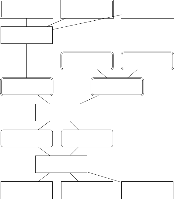
Figure 1 shows the high-level relationships between layers, core classes, and compilers. For layers,

there are two types: service layer and base layers. Service layers install service onto a single node. They

are rectangles with sharp edges and double borders in the ﬁgure. The scope of changes made by a service

layer is generally limited to a single node. Note that service layers do not make changes directly to

the core node classes. Instead, they make changes to “virtual nodes,” and the “virtual nodes” are later

bound to the core “Node‘ class, or a “physical” node. The reason for this will be discussed in the later

sections.

Base layers make changes to the entire emulation. Examples of this are the routing protocols, which

will involve changes on multiple router nodes, and the base layer, which itself creates hosts and routers

in the emulation. The base layers are rectangles with rounded edges and double borders in the ﬁgure.

The layers pass through the renderer to be converted to node and network objects. Node and network

objects are the core class objects; they are the single border, rounded edge rectangles in the ﬁgure. The

core class objects then pass through the compiler to become the “runnable” emulation.

Note that Figure 1 is only an overview, and therefore, only some available layers are shown. The

SEEDEMU oﬀers many layers to facilitate diﬀerent needs.

3.2 Enabling sharing and re-use of the emulations

One major consideration when the framework was designed was to enable users to re-use part of the

emulation. Which such a mechanism, one can share with others the emulation they built, or use the

emulations others had built in their own emulation.

In order to support the sharing feature, I came up with the following guidelines:

• Emulations should be separated into diﬀerent logical parts, where there are no hard-coded depen-

dencies and references between them. Each part should be able to function on its own, without

relying on other parts, during the emulation construction step.

• The emulation parts, either as code or as some dump ﬁle, should be imported and exported from

existing emulations easily.

• The emulations parts must be able to merge seamlessly should there be no conﬂicting deﬁnitions in

them. If there are conﬂicting deﬁnitions or conﬁgurations, the user should manually resolve such

conﬂicts, either with code or by interacting at run time with the framework.

In order to support the abovementioned guidelines, the following design decisions and features were

introduced to the framework:

Layered design. The emulations will be built from diﬀerent components called layers. Consider the

layer as the layer in the image editing software; each layer contains part of the information about the

emulation. Examples of layers are the base layer which stores information about what hosts and networks

are in the emulation, what networks they connect to, and more; the BGP layer, which describes how

autonomous systems have peered with each other; and the DNS layer, which stores information about

DNS zones, and what zones are being hosted on what host, etc. Each layer will only “mind their own

business,” in a sense that they only keep track of changes they want to make on the emulation - like

keeping an internal blueprint of the emulation. The changes are only committed to the emulation during

the render stage, where all the layers are “rendered” into one single emulation.

Binding and virtual nodes. As stated in the guideline, no hard-coded dependencies and references

between components (will be called “layers” from now on) are allowed. Layers that install services, like

the DNS layer, however, need to know what node in the emulation (will be called “physical node” from

now on) to commit their internal blueprint on - basically, what physical node to install and conﬁgure

the service on. In order to archive this, the binding and virtual node mechanism is introduced. A virtual

node is merely a string, a name text in the layers that would like to make changes to some physical

nodes. These layers track the changes they would like to make to diﬀerent physical nodes, identiﬁed by

the virtual node name, internally. Then, a set of rules can be deﬁned for each virtual node name to map

them onto the physical node.

Merging In order to allow the merging of an existing emulation with another emulation, the merging

feature is introduced. In case there are no common layers shared between two emulations, the merging

process is trivial. However, if two emulations contain the same type of layers, the merging will need some

special attention. Consider the case where there exist two DNS layers with diﬀerent zones conﬁgured in

them. In order to solve this, the framework allows users to implement mergers, where users can request

the emulation to pass two objects of the same type to the user for further merging operations. A set of

default mergers is included with the framework, which will try its best to merge two layers.

3.3 The core classes and interfaces

The core classes are the lowest-level representations of emulation objects. They are the direct abstractions

of the components in the lower-level emulation platforms. For example, the Node class may resemble

a service (i.e., a container in docker) or a virtual machine. The Network class may resemble a Linux

bridge. The Interface may resemble a Linux veth, a SR-IOV NIC, or even a physical NIC. It is up to

the compiler to “compile” them into their ﬁnal form on the target emulation platform.

For all the core classes, some APIs are provided to allow one to make changes to those objects.

The core classes cannot represent their real-world counterparts fully, and in fact, they never meant to.

Features provided by the core classes are carefully selected to work well under the context of for-education

emulation.

3.3.1 The Node class

The node class represents a computer, a server, a router, or any device that has Internet support. In

the SEEDEMU framework, a node is assumed to be a generic Linux host running a Debian-based distro.

The node class has APIs to allow one to do the followings:

• Connect to a network: Connecting to a network or other nodes is the essential feature of a node

that connects to the Internet.

• Adding ﬁles to node: There is also API to allow one to add ﬁles onto the node. Having this API

enables many emulation features, like adding conﬁguration ﬁles onto nodes.

• Add commands to run when “building” the node: In order to make a generic node running Linux

into a node that performs some role in the emulation, one may need to run some commands on

the node. One such example is running commands to install some software. The API to add build

command allows one to customize nodes to have any features they want.

• Add commands to run when the node starts: While adding commands to nodes during build time

allows one to customize the node, it is necessary to have the ability to add commands to run when

a node starts too. For example, on a router node, the routing daemon needs to be started when

the node starts, and on a client node, one may want to make it ping or curl to some other node

when it starts. The API to add start commands is therefore added.

These APIs, while not able to represent the full feature of real-world hosts, have provided enough

customizability that enables the emulation of complex scenarios for education uses. Example usages of

the framework are discussed in the case study section. Note that one may also interact with the nodes

directly after the node starts by accessing the console of the node directly. Therefore, it is not strictly

necessary to add everything one wants to run as start commands. Since the node is just a regular host

running Linux, one may also make changes to it that are not provided by the API. It is even possible to

have real-world computers join the emulation and appear to be a node in the emulation. These features

are discussed in the later sections.

3.3.2 The Network class and the Interface

The network class represents an Ethernet network. It can be considered as a switch, where nodes can

connect to. A network can be an Internet exchange, a part of some backbone, or just an internal LAN

network. On the network class, there is one API to allow one to enable remote access from the real world

to the network, usually by means of hosting a VPN server that is accessible from the real world. Details

of the real-world feature are in the real-world section.

An interface object connects a node to the network. The interface class has the APIs to allow one

to do the followings:

• Change MTU: More and more real-world Internet providers allows the use of the jumbo frame.

Having the API to set MTU allows the framework to handle those aspects of the Internet. Some

SEEDEMU features, like the MPLS layer, use this API, since they introduce layer two header

overhead.

• Set link emulation properties: There are APIs on the interface class to allow one to change the

link properties. These properties include link speed, packet drop probability, and max bandwidth.

This provides another important aspect of real-world networks.

• Setting the “direct” attribute: Networks that have “direct” attributes are learned by the routing

daemons and sent to BGP peers. Details of this design are described in the base layer and routing

section.

Again, the goals of these APIs are only to provide enough customizations, so it matches with

the previously set goals - for-education network emulation. And, even if some customizations are not

available, one can always enter the console of the nodes and perform the customizations manually.

3.4 The Emulator class

The Emulator class houses the core services one may need to work with building the emulation.

• Hooks: The emulator class provides hooks. Hooks allow one to hook onto various stages during

the rendering process to make changes to the emulation. The hook feature allows one to make

changes to the layer’s behavior without modifying the layer implementation.

• Bindings: Bindings allow one to bind virtual nodes to physical nodes. Virtual nodes are nodes

used in service layers to keep track of services to install and the conﬁguration ﬁles. Virtual nodes

are bound to physical nodes during render. This decouples node references and allows service layers

to operate on their own without base layers. Details about bindings are in the binding section.

• Virtual physical node: When a virtual node is created, one may want to make some additional

changes to the physical node that it is about to bound to. However, the physical node may not

even exist yet. The virtual physical node allows one to make changes to a real physical node object.

The changes made to that virtual physical node are then copied to the actual physical node upon

binding. Details about virtual nodes are in the virtual node section.

• The object registry: The object registry is where all objects in the emulation are stored: layers,

nodes, networks, hooks, and everything. One emulator class has only one object registry, storing

all objects in the emulation.

• Merging: The emulator class has a merge method to allow one to merge an emulation with another

to create a new emulation. This allows one to re-use emulations built by others. Details about the

merging feature are in the components section.

• Dumping and loading emulations: Dumping allows one to serialize the entire emulation into

a single binary ﬁle for easy sharing. Loading loads serialize the single binary ﬁle back into an

emulator object. Generally, this is used with the merging feature to share and re-use emulations.

Details about the dump and load feature are in the merging section.

• Service Network: A service network is a special network that has access to the real-world

Internet. The implementation of the service network depends on the compiler; the API merely

creates a network with a special type telling the compiler that this network is not an emulated

network, but is a network that should have access to the real-world Internet. This is used to support

various import features like VPN access for real-world hosts to connect to the emulated network

from the outside world, and NAT access for the hosts inside emulation to access the real-world

Internet. Details about the service network and service node are in the real-world section.

• Rendering and resolving layer dependencies: Naturally, one would want the base layers to

ﬁnish conﬁguring the emulation before other layers since no node exists before the base layer does

the conﬁgurations. The emulator class automatically learns and checks the dependencies of the

layers. The rendering logic is also handled by the emulator class. Details about rendering logic are

discussed in the rendering section.

3.5 The object registry

The object registry is a class to store objects in the emulations. All objects, including the core classes,

layers, hooks, and bindings, are stored in the registry. Every object registered in the registry will have

three keys to identify them. Namely, the scope, type, and name. Generally, the scope deﬁnes the owner

of the said object, the type deﬁnes the type of the object, and the name deﬁnes the name of the object.

For example, a router named router0 node belongs to AS150 will have a scope, type, and name value

of 150, rnode (router node), and router0.

Some objects registered in the registry will also have their own equivalent of the name, type, or scope

ﬁeld as their class attribute or method. For example, node objects have ASN attribute, which is also

used as its scope, node role attribute, which corresponds to the type, and name attribute, will be used as

its name. Those equivalent attributes are maintained by the object itself, so in theory, those attributes

can be diﬀerent from how they are registered in the registry. However, all objects created by layers or

other bulletin emulation functions will keep the attributes on the object itself and the attribute used

for the registry the same. Unless one builds an emulation without using layers and explicitly registers

objects in an odd way, the attribute will be consistent.

3.6 Layers

The layer is one of the most critical concepts and components in the SEEDEMU framework. The diﬀerent

functionality of the emulator is separated into diﬀerent layers. The base layer, for example, describes

the base of the emulation:

• what autonomous systems and Internet exchanges are in the emulator,

• what nodes and networks are in each of the autonomous systems,

• how nodes are connected with networks

BGP layer, on the other hand, describes how autonomous systems and where are peered with each

other, and what is the relationship between the peers.

Layers themselves are like helper tools to create and make changes like installing new software, or

adding conﬁguration ﬁles for the said software, on the core class objects (the intermediate representa-

tions). While one can technically create an emulation without using any of the layers and by manually

creating and updating the core class objects themselves, just like in any other network emulation software

and framework, the layer is one of the most important features that make the SEEDEMU framework

diﬀerent.

3.6.1 Base layers and service layers

The SEEDEMU framework classiﬁes layers into two diﬀerent categories. The ﬁrst category is the base

layers, and the second category is the service layers.

Base layers, not to be confused with the base layer, which is one of the base layers, make changes to

the emulation as a whole. A base layer makes changes to the entire emulation (like BGP, which conﬁgure

peeing across multiple diﬀerent autonomous systems, exchanges, and routers), and routing, which will

conﬁgure routing protocols, loopback addresses on all router nodes. The characteristic of base layers is

that they provide the basics to support the emulation and higher-level layers.

In contrast, service layers will typically only make changes to individual nodes. Examples of service

layers are the web service layer, which allows one to install web servers on nodes, and the DNS layer,

which allows users to host DNS zones on nodes. While the service layer is the type of layer that interacts

with a single node to install service on them instead of making changes to the entire emulation as a

whole, service layers can also have their internal “global” state. For example, the DNS layer keeps an

internal tree structure for DNS zones. Individual zones can be hosted on a single server (node-speciﬁc

data), but the zone structure itself is an “global” data of the DNS layer. The DNS layer uses the zone

tree to build appropriate NS records to aid the creation of the complete DNS chain, enabling one to

build a DNS infrastructure easily.

Design changes in diﬀerent iterations In the early iteration of the SEEDEMU framework, services

are installed by providing the node object to the services. This leads to one major problem. Referencing

other objects in the emulation means that it would not work if one were to use this same piece of code in

another emulation. This contradicts the early guideline, where each emulation component should have

no direct code dependencies on other codes for portability. Two new mechanisms, namely the virtual

node and binding mechanism, are introduced to solve this problem.

In this new design, layers must not directly reference objects that do not belong to themselves.

Instead, layers retrieve nodes from the registry, using the names and install services that way. It soon

ﬁnds that this design still has some downsides. One will have to know the names of objects in the other

layers for this to work, which is less than ideal, as one may get the lower layers from someone else and

may not have the details, like names of objects, that exist in the lower layers. One approach to this

problem is to have the users inspect the imported layers themselves to ﬁnd out the said details. Such an

approach, however, still does not oﬀer a seamless experience for users. This leads to the development of

the virtual node and binding system.

3.6.2 Virtual nodes, bindings, and conﬁgure-on-render

Three new mechanisms, namely the virtual node, binding, and conﬁgure-on-render mechanism, are in-

troduced to further increase the portability. The general idea is that, ﬁrst, the layer must not use any

node object to identify which node to install the services on, as that creates dependencies to the base

layer, as mentioned in the previous paragraph, and second, specifying the name of nodes in the lower

layers should not be the only way users can use to install service on a node.

Virtual node. As explained in the earlier section, the virtual node is the mechanism to enable services

to track changes they would like to make to a node. This virtual node name is only signiﬁcant to the

service.

Binding. A binding allows one to set how the virtual node gets bound to a physical node, using a set

of optional predicates, like ASN, IP, name, network preﬁx, of the node. Users may also supply their

functions to do the tests to elect a physical node for a virtual node. It is also entirely optional for set

predicates. If no predicates are given, the virtual node will be bound to a random available physical

node. Alternatively, should no physical nodes match the given predicates, the user can ask the binding

system to create a node that matches the given conditions. This enables one without any knowledge

about the lower layers to add new services with trivial eﬀorts.

Virtual physical node. A virtual physical node is an actual node object instance. Since the virtual

nodes are only bound to a physical node after the render process, if a user would like to make some

changes to that physical node, they would need to wait after the render process. Waiting, however, may

not always be an option. If a user is developing a component (a partial emulation that can be “plugged”

into another bigger emulation to form a full emulation; will be discussed in detail in the later sections.),

they would never have the chance to render the emulation themselves. In order to enable making changes

to physical nodes, in this case, the framework oﬀers a “virtual physical node” mechanism. The virtual

physical node provides a way for users to interact with the physical node by creating an actual physical

node object. Users can make changes to this imaginary physical node (with some limitations. Adding

new network interface cards, for example, are not supported.). The emulator will keep track of those

changes and apply the changes to the real physical node when the binding happens.

Conﬁgure-on-render. In order to take the portability one step further, the conﬁgure-on-render mech-

anism is introduced. This means layers will keep track of changes they planned to make internally and

only actually commit those changes during the render stage. This further allows layers to operate on

their own. With this mechanism, users can do operations like building services and conﬁguring BGP

peerings without the base layer. The design of this mechanism will be discussed in the later sections.

3.6.3 The binding system

Services are installed onto the virtual nodes. Virtual nodes are just a name that exists only inside the

service layers. The binding system is the system that allows one to “bind” a virtual node onto the

physical node, so the service can actually be installed onto the node. A binding consists of the binding

target, the binding ﬁlters, and the binding action.

Binding target Binding targets deﬁne the “target” virtual nodes of this binding. It can either be the

full name of the virtual node or a regular expression to test the name of the virtual node. The binding

will further evaluate virtual nodes that match the target. Otherwise, the binding system will skip to

the next binding in the bindings list. By oﬀering the option to use regular expressions, one can match

multiple virtual nodes and apply the same binding rules to them. This is found to be extremely useful

when deploying some services. For example, one can preﬁx all virtual nodes with web services with web-,

and match all those nodes with a single binding using web-.* as the target. While the binding targets

may match multiple virtual nodes, each node is bound individually by evaluating the ﬁlters and actions.

Binding ﬁlters Binding ﬁlters allow one to deﬁne a set of rules that the physical node must match in

order to be considered a binding candidate for the virtual node. SEEDEMU framework oﬀers some of

the most commonly used predicates in the binding ﬁlters:

• asn: The asn option allows one to narrow down physical nodes by their autonomous system

number. Useful if one wants their service to be deployed in a given autonomous system.

• ip: The ip option allows one to match against the IP address of the node.

• prefix: The prefix option allows one to match against the IP address on nodes using a preﬁx.

The preﬁx does not have to match the preﬁx on the interface of the node. As long as the preﬁx

given in the ﬁlter includes the node’s IP address, the node will be considered a candidate.

• nodeName: The nodeName options allow one to match against the physical node name. In diﬀerent

autonomous systems, physical nodes can have the same name. So if one created nodes name web

in diﬀerent autonomous systems and wants to host web services in all those autonomous systems,

they can use the node name option.

• custom: The custom options allow one to do their own matching. The options accept a function,

the virtual node name and the physical node object will be passed into the function, and the

function can return True to make the physical node a candidate. This allows one to have complete

control over the ﬁltering process.

• bound: The bound option tells the ﬁlter to also consider the physical nodes that already have a

virtual node bound to them as a candidate. By default, this option is False, meaning only physical

node that has not been bound will be considered. However, sometimes it may be useful to install

multiple services on the same node, given that they do not conﬂict with each other, and thus this

option.

With the default values above, if no rules are given, then that means all physical nodes that have

not been bound to virtual nodes are considered a candidate. This default means if one does not care

where their service will end up at, and simply want the service to be deployed, they can create a binding

that matches all virtual nodes (target = *, with an empty ﬁlter). This enables one to deploy services on

to emulation without knowing the underlying topology at all.

If multiple predicates are given, the physical node must match all of them in order to be considered

a candidate.

Binding actions Binding action allows one to set what action to take to select the physical node to

use from the list of candidates. There are four types of actions:

• First: uses the ﬁrst candidate.

• Random: pick randomly in the list.

• Last: pick the last candidate.

• New: The new action is, in fact, a special action. When one uses the new action, instead of selecting

nodes from existing physical nodes using the given ﬁlter, the binding system tries to create a new

physical node that matches the ﬁlter options.

Dynamically created nodes When one uses the “new” action in the ﬁlter, the binding system will

try to create a new physical node matching the given condition. This is useful when one wants to deploy

their services on an emulation that already has other services running. In such a case, there may not be

enough free physical nodes for installing the service. For example, when action new is used without any

ﬁlter options, the binding system will pick a random autonomous system, have the node join a random

internal network, give it a random name, and use that node for the virtual node. If an IP address is

given, it will try to ﬁnd the network that includes the given IP addresses and create a new physical node

in that network. However, the binding system will fail if the rules given cannot be satisﬁed without

creating a new autonomous system or new network. The binding system can only create new nodes and

nothing else.

3.7 Rendering

Rendering is the process where the “magic” happens. In the rendering stage, the render and conﬁgure

methods on each layer are called based on the order of their dependencies. The reason to have two stages

(render and conﬁgure) for render will be discussed later. The Emulator object, which allows the layers

to obtain information about the layer, is passed to the render and conﬁgure methods to allow layers to

make changes to the emulator and build the emulation scenario collaboratively.

In order to build the emulation, the layers need to work with each other by creating new and making

changes to the core classes objects in the global object registry and sharing other layers the details that

may be useful to the emulation building adding metadata to global object registry.

However, some layers need to be conﬁgured and rendered so that the other layer can easily work

with the emulator. For example, for the BGP layer to conﬁgure peering of the autonomous system across

an Internet exchange or a cross-connect connection, the base layer must have ﬁrst created the router

nodes in those two autonomous systems and the network for the Internet exchange or cross-connect.

Intuitively, this issue is named layer dependencies.

3.7.1 Layer dependencies

In order to solve the issue of layer dependencies, the layer provides four diﬀerent types of dependencies

conﬁgurations:

Forward dependencies. The forward dependencies are the most common dependencies. For example,

nearly all layers have a forward dependency on the base layer. Since if no nodes register in the emulation,

there is nothing a layer can work on.

Inverse dependencies. The inverse dependencies are the dependencies where a layer wants to ensure

the other layer to be rendered after itself, but that target layer may not know the existent of the said layer

creating this dependency. Moreover, since there is no way to register new dependencies after the layer is

created, the inverse-dependencies mechanism is introduced to allow a layer to add itself as a dependency

of another layer. An example use of the inverse-dependencies mechanism is the zone-generating layers.

Zone-generating layers, as their name suggested, generate DNS zones. They allow users to add descriptive

reverse DNS hostnames to IP addresses in the emulation. The zone-generating layers need to be rendered

before the DNS layer ﬁnalizes its zone and generates the zone ﬁle output to the DNS server nodes since

making changes are not allowed after the render stage (this will be discussed in the layer lifecycle section

below).

Optional forward and optional inverse dependencies. Another case of dependencies is the op-

tional dependencies. A layer may want another layer to be rendered before or after itself but also want to

allow the render and conﬁguration process to continue even if the said layer does not exist. The optional

dependency is a less common use case. An example of optional dependencies is the MPLS layer. MPLS

declares itself to be the optional inverse dependency of the IBGP and OSPF layers. This is because the

MPLS layer replaces the job of both layers, and MPLS needs to ensure IBGP and OSPF layer does not

interfere with an MPLS-enabled autonomous system by masking the autonomous system from IBGP

and OSPF layer.

3.7.2 Layers lifecycle and conﬁgure-on-render

One major mechanism of the SEEDEMU framework is the conﬁgure-on-render behavior, also known as

the lazy-create policy. The core class objects are not created or modiﬁed unless the user initiates a render

call. This ensures that layers will not have access to other emulator components prior to the render,

eliminating antipattern designs from the root.

The rendering process is broken into two parts. Namely, render and conﬁgure.

Layers will have no knowledge of what or how other layers are conﬁgured prior to the render stage.

Therefore, layers must keep track of the changes they try to make internally within the class. The process

Layer created

Layer ready

Layer conﬁgured

Layer ﬁnalized

User calling methods on the layer class

Renderer calling the conﬁgure method

Renderer calling the render method

Figure 2: Layer lifecycle

of actually making changes, like adding nodes, networks, peering conﬁgurations, or other features like

DNS, web server, and more, into the emulation, is called rendering.

During the render stage, the render method of each layer will be called in order of their depen-

dencies, and the Emulator object will be passed in. The Emulator object allows the diﬀerent layers to

collaboratively build a single emulation by providing access to other objects in the emulation.

Conﬁguration is an optional step. In the conﬁguration stage, layers will also be provided with access

to the Emulator object. The conﬁguration stage allows the layer developer to have more control over

the emulation construction. During the conﬁgure stage, layers can register the data that other layers

might need. For example, the base layer registers the nodes, networks and resolves all pending network

joins. Layers, however, are designed to not make ﬁnal changes during the conﬁgure stage, as there are

chances that other layers will add new data to the emulator. The conﬁguration stage is especially useful

if a layer wants to make changes to another layer but still requires the other layer to have conﬁgured the

emulator ﬁrst. Currently, this is used in the ReverseDomainName and CymruIpOrigin service, both of

which create a new zone in the DomainName service. They do so in the conﬁgure stage, as DomainName

would have already compiled the Zone data structure to zone ﬁles in the render stage, and additional

zone added after the render stage will not be included in the ﬁnal output.

One important reason to use the conﬁgure-on-render mechanism is that it forces the layer developer

to not reference any object outside its class, by names of by references, before the render. This means

layers can be easily taken out of their current context and put into another emulation. This also allows

layers to operate solely on their own - the object it references does not need to exist at the emulation

construction time. As long as the object exists during the render stage, the layer will work just ﬁne.

Another important point to know is that the conﬁgure-on-render mechanism does not forbid making

changes to layers after the render ﬁnishes; it merely suggests that layers must accept changes prior to the

render ﬁnishes. Having such guidelines simpliﬁes the work for both the layer developers and the layer

users. With such guidelines, the layer developers know when they can safely ﬁnalize the layer, and users

also know that if they were to make changes prior to the render, the layers would note the changes. The

full lifecycle and ﬂow of the layers are shown in Figure 2.

3.7.3 Rendering ﬂow

Function Render():

ResolveBindings();

if HasUnresolvedBindings() then

/* Error out. */

return 1 ;

end

/* Stage 1: configure all layers. */

for layer in layers do

ConfigureLayer(layer);

end

/* Stage 2: render all layers. */

for layer in layers do

RenderLayer(layer);

end

/* Recursively configure a layer and its dependencies. */

Function ConfigureLayer(layer):

if IsConfigured(layer) then

continue;

end

for dep in layer.dependencies do

ConfigureLayer(dep);

end

InvokePreConfigueHooksFor(layer);

layer.Configure(emulator);

InvokePostConfigueHooksFor(layer);

/* Recursively render a layer and its dependencies. */

Function RenderLayer(layer):

if IsRendered(layer) then

continue;

end

for dep in layer.dependencies do

RenderLayer(dep);

end

InvokePreRenderHooksFor(layer);

layer.Render(emulator);

InvokePostRenderHooksFor(layer);

Algorithm 1: Rendering ﬂow

Rendering is the process of requesting the various layers in the emulation to convert the internal

conﬁguration and data structures to the core-class objects (i.e., the intermediate representations of real-

world components like networks, computers, routers, and more). Rendering is s multi-stage process. The

detailed rendering workﬂows are described in algorithm 1.

The rendering process will ﬁrst try to resolve all bindings, with the process detailed in the binding

section. If some virtual nodes cannot be resolved with the bindings provided, the rendering process

will error out and let the users know the details. The overall workﬂow for the render and conﬁgure

stage is the same. Both processes will iterate through all layers within the emulation. For each layer,

the renderer will invoke a recursive function to render the layer and dependencies of the layer. In the

recursive function for render and conﬁgure, they ﬁrst check if the layer is rendered or conﬁgured. If

not, they iterate through all layer dependencies and recursively call the render and conﬁgure on the

dependencies.

The renderer also oﬀers the “hook” feature. Users can “hook” into the various steps of the rendering

process, namely pre-conﬁguration, post-conﬁguration, pre-render, and post-render, and perform custom

actions. To add a new hook, the user would need to create a new Hook class instance. The Hook class

instance will contain the name of the layer to target and the step (pre-conﬁguration, post-conﬁguration,

pre-render, and post-render) to target. Multiple hooks for the same layer and the same step can be

added. The renderer will invoke the user-deﬁned hooks during the appropriate stage in the rendering

process and pass the emulator object to the user-deﬁned function. The hook mechanism is useful if the

user wants to make some changes to the layer behavior but does not want to change the layer code.

3.8 Components: sharing emulations

One other major feature of the SEEDEMU framework is the ability to reuse already built emulation in

another emulation. In order to enable easy reuse, besides having all components working independently,

some mechanism enabling easy export and import of emulation is needed. While one can copy and paste

code to “share” the emulation, the framework oﬀers two more ﬂexible options, emulation import/export,

and component classes, to facilitate easy sharing of the emulations.

3.8.1 Emulation import and export

The easiest way one can share an emulation is through the Emulator::dump and Emulator::load API.

The dump API will dump all information in the emulation (the global object registry, the bindings, the

layers, the hooks, and more) into a single ﬁle. The load API, in turn, reads the dumped objects back

into the emulator. The dump ﬁle is the emulation serialized into a single binary ﬁle. The serialization

and deserialization are accomplished with the python pickle library.

The dump API only supports dumping not-yet-rendered emulations, as its sole purpose is to facilitate

sharing the “parts” of emulation. The “parts” are supposed to use to build a bigger emulation. Since no

changes can be made after the emulation is rendered, it does not make sense to allow dumping emulations

that are already rendered.

The load API overrides all the changes on the calling emulator object, so one should not make

changes to the emulator object prior to loading dumped ﬁles. The recommended approach is to create

a new emulator class instance, invoke the load method, then merge the new emulator instance and the

old emulator instance with the merge API. The merge API is discussed in the later section.

3.8.2 Component classes

One of the drawbacks of sharing emulations using the dumped ﬁle is that there are only limited options

to customize the imported emulation. The SEEDEMU framework oﬀers the Component interface as

a guideline as to how one can create a sharable and customizable emulation “part.” Consider the

component interface as a “emulator factory class.” They produce new emulator objects with the given

conﬁguration options. One example of the component class is the BGP hijacker component, allowing

users to set the ASN, preﬁx to hijack, and exchange to join. The hijacker component will generate an

emulator will the appropriate base, routing, and BGP layer to support the hijack scenario. The user can

then use an API to get the emulator and merge it with the emulation they are building.

There is only one method, get, required on the component interface. The get method needs to

return an emulator object. One would call this method if they want the actual component to be merged

with their emulator.

3.8.3 Merging emulations

The Emulator::merge method tries to merge two emulators. It merges the current emulator with

the given emulator and returns a new, merged emulator. It merges the bindings, hooks, virtual node

deﬁnitions, and layers. However, in some cases, one may merge two emulations that contain the same

type of layer. There needs to be some way to handle the merging of the layers. In order to solve the

merging problem, the merger mechanism is developed. When one invokes merge, they optionally pass in

a list of mergers to handle to merging of the layers. Furthermore, a set of default mergers is provided to

support the common merging case of the commonly used layer.

Default base layer merger The logic of the default base layer merger is that it will try to merge

two base layers with no overlapping Internet exchanges and autonomous systems. If there are conﬂicting

autonomous systems or Internet exchanges, the autonomous system or Internet exchange in the ﬁrst

emulation will be used. The user can optionally supply a callback function to handle the merging of the

autonomous systems and Internet exchanges.

Default service layer merger All the service layers share a common property, the pending targets.

A shared service merger interface is provided to help to merge these service layers. Most of the service

needs no additional logic to handle the merging. They only need to implement the createService

method to return a new instance of the service to serve as the container of the merged service.

Default BGP looking glass service merger The BGP looking glass service uses the service merger

interface and has no additional logic to it.

Default Cymru IP origin service merger The Cymru IP origin service merger uses the service

merger interface and merges the manually created DNS records.

Default DNSSEC layer merger The DNSSEC layer merger merely merges the list of DNSSEC-

enabled domains.

Default DNS caching service merger The DNS caching service merger uses the service merger

interface and has no additional logic to it.

Default DNS service merger The DNS service ﬁrst uses the service merger interface to merge the

targets, then recursively merges the zone trees in the services. It errors out if a domain name is a zone

in one service and a record in the other service.

Default EBGP layer merger The EBGP layer merger merges all peerings (Internet exchange peer-

ings, route server peers, cross-connect peerings). For the Internet exchange peerings and cross-connect

peerings, if the peering relationship in two layers for the same peering diﬀers, the relationship in the

ﬁrst emulator will be used. Users may supply a callback function to handle the merging for when the

relationship diﬀers.

Default IBGP layer merger The IBGP layer merger merges the list of masked autonomous system

numbers in the two layers.

Default MPLS layer merger The MPLS layer merger merges the list of MPLS-enabled autonomous

system numbers and manually deﬁned edge routers in the two layers.

Default OSPF layer merger The OSPF layer merger merges the list of masked autonomous system

numbers and networks and stubnets in the two layers.

Default reverse domain name services merger The reverse DNS service merger uses the service

merger interface and has no additional logic to it.

Default routing layer merger The routing layer has no conﬁgurable options. The merging operation

is just to create a new routing layer.

Default web services merger The web service merger uses the service merger interface and has no

additional logic to it.

4 The base layers

Not to be confused with the base layer, “base layers” is the name of the type of layers. The base layers

are a group of layers that servers as the base of the emulation. One of the most important roles of base

layers is to provide layer two connectivity and layer three routing between all nodes in the emulation.

Not to be confused with the base layer, which is the layer that provides the APIs for one to create

Internet exchanges, autonomous systems, hosts, and networks.

4.1 The base layer

The base layer helps one create layer two topologies in the emulation. It enables one to create autonomous

systems and Internet exchanges quickly. It also handles conﬁguring network interfaces. (renaming

the interface from genetic names like eth0 to net0 (the name of the network in the emulation), and

conﬁguring tc rules to emulated latency, packet drops, and more) The base layer provides API to:

• Create autonomous systems: Since the emulator aims for Internet emulation, it is logical to have

nodes and networks belonging to autonomous systems. The API allows one to create a new

AutonomousSystem instance. The instance helps one create and manage routers, hosts, and net-

works in an autonomous system.

• Create Internet exchanges: Internet exchanges are a special type of network that allows routers

from diﬀerent autonomous systems to connect to. It is the essential feature that enables routing

across autonomous system boundaries.

4.1.1 Renaming interface

Base layer renames interfaces from their original names like eth0 or enp2s0 into names that represent the

network they connected to, like net1. Depending on the emulation platforms, the interfaces may have

diﬀerent names and orders inside the emulation node. Renaming them into the name of the connected

network guarantees that they will have the same name. This greatly simpliﬁes the job of all routing

layers. For example, with the interfaces renamed, enabling OSPF for a network is to add an entry to the

OSPF-enabled interface list using the network name as the interface name. Using the name means this

conﬁguration can be easily generated at compile-time instead of ﬁguring out and ﬁlling in the interface

names at run time.

4.1.2 Examples

APIs of the SEEDEMU framework are created with ease of use in mind. Below are code snippets showing

how one can create a basic stub autonomous system and Internet exchange.

Creating Internet exchange As shown in listing 2 with just one line of code, a new Internet exchange

is created. Routes from diﬀerent autonomous systems can later join the exchange using the joinNetwork

call.

Listing 2: Creating and joining an Internet exchange

base.createInternetExchange(100)

Creating autonomous system With merely six lines of code, one can have a simple stub autonomous

system up and running. Listing 3 shows the full process for creating an autonomous system with one

router, one network, and one host running a web server. Details of the binding system and virtual nodes

are discussed later.

Listing 3: Creating a stub autonomous system

# Create an autonomous system

as150 = base.createAutonomousSystem(150)

# Create a network. By default, networks created have the "direct"

# attribute and will be sent to BGP peers so that they are reachable

# from other hosts within the emulation.

as150.createNetwork('net0')

# Create a router and connect it to two networks

as150.createRouter('router0').joinNetwork('net0').joinNetwork('ix100')

# Create a host called web and connect it to a network

as150.createHost('web').joinNetwork('net0')

# Create a web service on virtual node, give it a name

# This will install the web service on this virtual node

web.install('web150')

# Bind the virtual node to a physical node

emu.addBinding(

Binding('web150', filter = Filter(nodeName = 'web', asn = 150))

)

4.2 The routing layer

The routing layer is a “hidden layer,” because it does not provide any conﬁgurable options but is just

there to provide the support for other routing protocols. The routing layer will install the routing daemon,

BIRD [9], on all router nodes, create a dummy loopback interface, assigns loopback IP to all the routes,

and extend and create extension methods on the Node core class to allow adding new dynamic routing

protocols to the routing daemon. The routing layer also handles adding default gateway on non-router

nodes to point to the nearest router node connected.

4.2.1 Multiple routing tables

The routing layer oﬀers features to allow the use of multiple routing tables. The way that the other

routing layers use the multiple routing tables is that each routing protocol will store their routes in their

routing table. This will prevent unintentional route leaking from one protocol to another since one will

have to explicitly create pipes between routing tables to copy routes between routing tables. One such

example is OSPF. Generally, OSPF is not for handling a large number of routes, and therefore leaking

BGP routes into OSPF can cause performance issues and OSPF session ﬂapping.

4.2.2 Direct interfaces

The routing layer handles the direct ﬂag on networks. When a network has the direct ﬂag, the routing

layer will add it to the direct protocol in BIRD, which generates routes for the preﬁx of the IP address

on the interface. These routes are saved in the t direct routing table. Other routing protocols, like

BGP, can import these routes into their table and advertise them to peers. This is how internal networks

got announced to other autonomous systems in the emulator. The same practice is widely adopted in

the real world and oﬀers a realistic emulation of the real world.

4.2.3 The dummy interface and loopback IP

The routing layer will also add a dummy interface with a generated loopback IP address. The range of

loopback IP defaults to 10.0.0.0/16, as this network belongs to AS0, which is an invalid autonomous

system number according to the default network assignment scheme. One can override the network

block used for loopback IP addresses bypassing it in the loopback range parameter in the Routing

layer constructor.

This dummy IP address provides a unique loopback IP for every router in the emulation. The

loopback IP will only be reachable within the local network covered by the same OSPF domain by

default. It provides ease of conﬁguration and redundancy for the other protocols like LDP and BGP.

The way it works will be detailed in the respective sections. Note that this should not be confused with

the loopback interface lo and loopback IP address range 127/8.

4.2.4 The real-world integration

One other feature backed by the routing layer is real-world integration. The real-world integration

feature requires the corporation of the base layer, routing layer, and the compiler. The base layer will

need to create a special network and node with the “real-world” attribute. The “real-world” nodes are

nodes that are present in the emulation but do not participate in emulation. “Participate in emulation”

here means running services or routing protocols that allow interaction from other nodes within the

emulation. Instead, the “real-world” node sits in between the emulation and reality. They have access to

a “real-world” network, a special network that should provide Internet access to the outside world. They

may also have access to some emulated networks. They can route traﬃc from hosts inside the emulation

to the outside world or hosts VPN servers so that hosts from outside can join the emulated networks.

The former is usually done by announcing routes to other routers, and when traﬃc reaches it, it does

NAT to route traﬃc out. The latter is usually by creating some layer-two VPN and bridging the VPN

interface with the internal network.

Real-world hosts access the real-world node either utilizing port forwarding or having the real-world

have a publicly accessible IP address. This is mainly to enable the real-world hosts to connect to the

VPN servers. Since how such a feature is implemented depends highly on the emulation platform, the

main job for making the feature works is on the compiler.

Hiding real-world hops One trick used by the SEEDEMU framework to hide real-world hops from

the programs like traceroute is setting TTL of packets to 64 for traﬃc destinating the real world. Since

traceroute uses low-TTL packets, setting TTL to 64 when sending traﬃc out will make the next-hop

router that was originally supposed to get a packet with TTL of one get a packet with high TTL instead,

and continue routing packet normally. From inside the emulation, it would look like that the actual

real-world host is just one hop away from the real-world router node. This reduces the confusion. The

hiding behavior is conﬁgurable so that one can disable this behavior should one want to.

Remote access providers In order to allow real-world hosts to connect to the emulated network,

VPNs are used. However, since users may have diﬀerent needs, and it is not feasible to develop all remote

access options to support every diﬀerent use case, the SEEDEMU framework uses a generic interface for

oﬀering remote access. The RemoteAccessProvider interface allows one to implement their own logic

to support remote access to emulated networks. The interfaces pass in the emulated network object,

the real-world node, and network object, and one can run and command they want on the real-world

node. One may even run a VPN client on the node that connects to other VPN servers on the real-world

node instead. The interface generalized the remote access feature and therefore opened up diﬀerent

possibilities.

4.2.5 Examples

Here are some code snippets demoing how one can enable remote access to the real world or route traﬃc

from the emulation to the real world. Complete examples are in the case study section.

Creating router that routes traﬃc to the real-world To route traﬃc to the real world, one would

just create a real-world router, connect it to an exchange, and have it peer with some other autonomous

system.

Listing 4: Snippet for enabling access to real-world

as11872 = base.createAutonomousSystem(11872)

as11872.createRealWorldRouter('rw').joinNetwork('ix101', '10.101.0.118')

ebgp.addPrivatePeering(101, 150, 11872, abRelationship = PeerRelationship.Provider)

Listing 4 shows all the API calls one would need to enable access to the real world. When one calls

createRealWorldRouter, the framework automatically fetches routes announced by the autonomous

systems in the real world. The auto fetch behavior can be disabled. One can also manually specify

routes they want to route to the outside. The createAutonomousSystem and joinNetwork call do the

same thing as demonstrated in the base layer snippet before. The addPrivatePeering call creates

private peering between two autonomous systems in the given Internet exchange. The details about

peering are in the next section.

Hosting VPN servers to connect real-world hosts to emulation Hosting a VPN server to allow

connection from the real world can also be done in a single API call.

Listing 5: Snippet for enabling access to real-world

as151 = base.createAutonomousSystem(151)

ovpn = OpenVpnRemoteAccessProvider()

as151.createNetwork('net0').enableRemoteAccess(ovpn)

as151.createRouter('router0').joinNetwork('net0').joinNetwork('ix100')

Listing 5 shows how one would enable remote access to an emulated network, net0 in AS151, for the

real world. The OpenVPN remote access provider will host an OpenVPN server that is reachable from

the real world. It uses a set of bulletin keys and certiﬁcates. A client-side conﬁguration ﬁle is included

with the framework. One may also have the server uses their own key and certiﬁcate pair. Details are

in the case study section.

4.3 The EBGP layer

The EBGP layers enable automatic external BGP peerings via Internet exchange route servers, private

sessions in an Internet exchange, and cross-connects.

4.3.1 How is it done in the real world?

BGP peerings Generally, real-world BGP peers are done over Internet exchanges, or private inter-

connects. An Internet exchange, at its core, is simply a layer two switch where all members connect to

it and peer with each other over the switched links. When two autonomous systems use private inter-

connects to peer with each other, they will set up a BGP session across the link. However, when the two

autonomous systems join the same Internet exchange, they may not set up direct peering. They may

peer via the route server or not peer at all. The route server sends routes received from one autonomous

system to all other autonomous systems connected to the route server, eﬀectively making a full-mesh

peering between all participants connected to the route server.

Autonomous systems may also have complex routing policies. For example, some may prefer routes

received over a private interconnect over an Internet exchange. Some may send diﬀerent routes to the

route server than peers with the direct session over Internet exchange.

Besides regular peering in Internet exchanges, autonomous systems can also have a provider-customer

relationship. A provider will send the full Internet routing table to their customers (or, sometimes, upon

customer requests, sends no route at all or only a default route to the customer.) and re-advertise routes

received from the customers to all its peer or even its provider - a provider can be another provider’s

provider.

ISP tiers When considering providers, it is a common practice to classify providers according to their

tier. However, the deﬁnition of transit provider tier is somewhat ad-hoc; generally, tier-1 transit providers

are providers that do not need to purchase any transit from other providers to reach the entire Internet. In

other words, tier-1 transit providers can reach the entire Internet with only peering. Tier-2 two providers

can access a large part of the Internet via peerings but still purchase services from tier-1 providers to get

the full connectivity. Tier-3 providers are the providers that rely mostly on other providers to reach the

Internet. While tier-3 can also join Internet exchange to have peerings, the peering routes usually only

consist of a small part of their connectivities.

The provider tier is merely decided by how many customers they have and if other tier-1 ISPs want

to peer with them. Generally, when a small group of ISPs can reach their part of the “Internet” (usually

because they have so many customers, some of which may even be tier-2 ISPs), but not the part of the

Internet of the other ISPs of the same scale. This group of ISPs can peer with each other and send all

their customer routes to each other free of charge. In this case, these ISPs become tier-1s. In theory, if an

ISP gains enough customers, and joins enough Internet exchanges, and has enough private interconnects

to reach the entire Internet, they can become tier-1 too. However, there are still a lot of other factors,

like if the other tier-1 would like to peer with one and send all their routes to one.

Peering relationships and route ﬁlters Generally, there are only two types of peering relationships.

The ﬁrst is the regular peering, where the autonomous systems send routes that belong to themselves or

their customers to the peer and do not re-announce routes received from peers to other peers. The other

relationship is a provider-customer relationship, where the provider sends all routes to the customer and

re-advertises the customer’s routes to other peers so that the world can reach the customer.

To ensure the peer or customers only send routes that belong to them or their customer, one will

usually apply route ﬁlters when importing routes from other autonomous systems. There are many

options to create route ﬁlters. In the real world, the most common option is to use the Internet Routing

Registry (IRR). IRR is a database that associates route preﬁxes with autonomous system numbers.

When peering with another autonomous system, one will generally send the other side their as-set. An

as-set is a set of autonomous system numbers. It is one type of object in an IRR database. From those

autonomous system numbers, one ﬁnds out route preﬁxes associated with those autonomous system

numbers and generates route ﬁlters based on the route object. A route object is also an IRR database

object. The route object associates a network preﬁx with an autonomous system number. There are also

sources of information besides IRR, like the Resource Public Key Infrastructure (RPKI) or just plain

human communication.

Route preferences While the BGP protocol has the AS PATH attribute and preferring the routes

with shorter paths seems straightforward and logical, for providers, they rarely use AS PATH as the most

signiﬁcant factor when picking routes. For starters, a longer AS

PATH does not necessarily mean the path

is actually longer or slower - it merely indicates that the routes have traveled through more autonomous

systems. It is also possible that some autonomous systems along the path prepended some amount of

autonomous system numbers to the path. Peerings can also happen over links with diﬀerent bandwidths.

A path with short AS PATH may lead to a saturated link or a link with low bandwidth. Solutions to these

problems vary - there are traﬃc engineering options to steer traﬃc away from the saturated links, there

are also some other ad-hoc optimizations to move routes based on packet loss, latency, and other ad-hoc

metrics.

However, the one method that is the most basic is the LOCAL PREF attribute of BGP routes. A route

with high local preference will always be preferred, no matter its AS PATH length. Generally, one will

give routes originated from oneself the highest preference, so the routes will not end up routing traﬃc

destinating oneself to other autonomous systems. The next preferred routes are generally the customer

routes, followed by the peer routes and provider routes. Customer routes are preferred over peer routes

and customer routes since the customer may multi-home with other providers. In such a case, traﬃc

should be sent directly to the customers instead of going through peers or transits, unless the customer

explicitly wanted to. And peer routes are usually more preferred than transit routes since transit routes

usually have a higher associated cost.

Large transit providers may also provide BGP communities to alter the route preference. Some

example of the communities includes “tag routes with (aaa:bbb) to set local-preference to XX in region

YY,” where XX is a number and YY is a region. This allows the customer to selectively alter routes in

a diﬀerent region. For example, if the customer has some anycast setup, they may want the provider

to prefer local peer routes instead of sending traﬃc back to where they purchase transit service. Other

control communities may also be available, like controlling the export to some target autonomous systems.

There does not exist a standard for BGP communities (other than the well-known no-export and

no-advertise community, and even the well-known communities may not be supported everywhere), as

each provider implements its own action communities.

4.3.2 EBGP in the SEEDEMU framework

The EBGP layer, at its core, is relatively simple. It checks every peering conﬁgured. For each Internet

exchange, it will loop through every connected node and conﬁgure peering accordingly. The EBGP layer

errors out if any given peering relationship cannot be satisﬁed. An unsatisﬁable peering relationship

generally means a cross-connection does not exist, one or both autonomous systems are not in the given

exchange, or the Internet exchange does not exist.

The SEEDEMU framework only deﬁnes three types of peering relationships and uses a set of default

preferences for the diﬀerent types of routes.

Peering relationships and routing policies The EBGP layer has deﬁned three types of peerings

relationships:

• Regular peer: In the regular peer relationship, both sides export their own routes and their

customer’s routes to each other. Routes imported from the other side are marked as peer routes.

• Provider-customer: In the provider-customer relationship, the provider side will export all routes

it has to the customer side (including its own routes, its peer’s routes, and other customer routes).

On the other hand, the customer side exports only its own routes and its customer’s route to the

provider side. When importing, the provider side marks the routes it learned from the customer

side as the customer route, and the customer side marks the routes it learned from the provider

side as provider routes.

• Unﬁltered: In the unﬁltered relationship, both sides export all routes to the other sides, and both

side marks the imported route as the customer route.

Note that in the BGP layer, BGP peers only enforce export policies. There is no ﬁlter applied when

importing routes from BGP peers. Since the ﬁlters are generated by the program, there will be no route

leak by default. This means if one wants to perform route hijack in the emulation or internally create

misconﬁgurations, they can easily do so. They simply need to export the route to their provider. The

real-world model of import-based ﬁltering, while working great in the real world, does not ﬁt in the

context of for-education emulations. Using export-based ﬁlters provides some degree of realism while

allowing one to create misconﬁgured scenarios and hijacks easily intentionally.

Figure 3 shows the route imported from seven diﬀerent peers of the four types. The direction of the

arrow indicates the direction of routes being sent. Assuming the routes originated by AS150 is s, the

Provider A

Peer C

Peer D

Provider B

AS150

Unﬁltered Peer E

Customer F Customer G

a’

b’ b

c’

d’

e’

f’ f

g’

Figure 3: BGP relationships and export ﬁlters

route exported to each peer are:

• Provider a = s + f

+ g

+ e

• Provider b = s + f

+ g

+ e

• Peer c = s + f

+ g

+ e

• Peer d = s + f

+ g

+ e

• Unﬁltered peer e = s + a

+ b

+ c

+ d

+ f

+ g

(i.e., everything expect the routes received from E)

• Customer f = s + a

+ b

+ c

+ d

+ e

+ g

(i.e., everything expect the routes received from F)

• Customer g = s + a

+ b

+ c

+ d

+ e

+ f

(i.e., everything expect the routes received from G)

In practice, for unﬁltered and customer sessions, there is no ﬁlter applied at all (i.e., export all;

in BIRD’s conﬁguration.). BGP, by default, will not send routes received from the peer back to the same

peer.

Route ﬁlters and BGP communities convention The EBGP layer ﬁlters route sent to BGP peers

with BGP communities according to the export policies deﬁned above. Routes are tagged with diﬀerent

BGP communities according to their source.

EBGP layer uses a variant of the BGP community [15], BGP large community [16]. In the early days,

people assumed 16-bit autonomous system numbers would be enough bit to support all networks [14].

However, very soon, the 16-bit autonomous systems numbers were nearly exhausted, and an extension

was added to BGP to allow 32-bit autonomous system numbers [17]. The old BGP community, therefore,

only supports a tuple of two 16-bit values. The BGP large community supports three 32-bit values [16].

In order to make sure one can use 32-bit autonomous system numbers with the EBGP layer, the EBGP

layer uses BGP large community to tag routes. In the EBGP layer, routes are tagged using the following

communities:

• Routes originated by the autonomous system itself are tagged with the large community asn:0:0,

where asn is the autonomous system of the current autonomous system.

• Routes received from the customers of an autonomous system are tagged with the large community

asn:1:0, where asn is the autonomous system of the current autonomous system.

• Routes received from the peers of an autonomous system are tagged with the large community

asn:2:0, where asn is the autonomous system of the current autonomous system.

• Routes received from the providers of an autonomous system are tagged with the large community

asn:3:0, where asn is the autonomous system of the current autonomous system.

These communities are then tested when exporting routes to other BGP peers. For example, if a

BGP speaker is exporting routes to its provider, it will only export those routes with one of the following

large communities:

• asn:0:0 (one’s own routes)

• asn:1:0 (customer routes)

Or, as a BIRD ﬁlter expression:

Listing 6: BIRD export ﬁlter

protocol bgp u_XXX {

ipv4 {

# ...

export where bgp_large_community ~ [LOCAL_COMM, CUSTOMER_COMM];

# ...

};

local 10.100.0.150 as 150;

neighbor 10.100.0.100 as 100;

}

Having the peering relationship and ﬁlter in place ensures an autonomous stub system does not

accidentally end up transiting other networks. Having the ﬁlters also sometimes creates suboptimal

forwarding paths - and just like the real world, those suboptimal forwarding paths are there because of

how providers peer and conﬁgure their network.

While ﬁltering based on only the BGP communities is rarely the recommended practice in the real

world, it is perfectly applicable in the context of for-education Internet emulation. Since the ﬁlters and

route tagging are done automatically by the EBGP layer, there are, normally, no possible route leaks or

route hijacks. However, should one want to create a route hijack or route leak scenario, they can easily

do so by adding the appropriate BGP community to the routes.

BGP communities also help one to identify how a route gets to the router. For example, when

inspecting the BGP table in BIRD, one may see something like this:

Listing 7: BGP routing table

bird> s rou 10.161.0.0/24 all

Table master4:

10.161.0.0/24 unicast [u_as3 18:15:48.130] * (100) [AS161i]

via 10.100.0.3 on ix100

Type: BGP univ

BGP.origin: IGP

BGP.as_path: 3 161

BGP.next_hop: 10.100.0.3

BGP.local_pref: 10

BGP.large_community: (3, 1, 0) (161, 0, 0) (150, 3, 0)

unicast [u_as2 18:15:48.131] (100) [AS161i]

via 10.100.0.2 on ix100

Type: BGP univ

BGP.origin: IGP

BGP.as_path: 2 3 161

BGP.next_hop: 10.100.0.2

BGP.local_pref: 10

BGP.large_community: (2, 2, 0) (3, 1, 0) (161, 0, 0) (150, 3, 0)

Listing 7 shows how a route may look like on AS150’s router. For the ﬁrst route, 3:1:0 indicates

that this route was received from a customer by AS3. By looking at the AS PATH, it is clear that this

route is received from AS161 by AS3. The community 161:0:0 means AS161 originated this route, and

150:3:0 is tagged by the AS150’s router itself (i.e., the current router) to indicate that the route is

received from a provider. For the second available path, 2:2:0 indicates that the route was received

from a peer (AS3 in this case, as seen in the AS PATH).

Default local preferences Default local preferences for routes imported from diﬀerent peer types are

as follows:

• One’s own routes: 40 (the highest). If a route belongs to the autonomous system itself, the route

will have the highest route preference, 40. This ensures that as long as any internal path exists for

a preﬁx that belongs to the same autonomous system, no external BGP peers’ routes will be used.

In other words, no traﬃc to the local networks will go through the emulated Internet.

• One’s customer’s routes: 30 (2nd). If there exists any route to a customer, the route will be used.

If the customer has more than one provider, other paths, via some other providers, to the same

preﬁx may be available. Setting a high preference for the customer ensures that as long as the

customer is sending routes, those routes will always be picked.

• One’s peer’s routes: 20 (3rd). Peer routes are the 3rd preferred routes. Generally, peerings are

settlement-free, and therefore routes from a peer are more preferred, as routing traﬃc through a

transit provider usually has some associated cost.

• One’s provider’s routes: 10 (4th). Routes received from the providers are generally the least

preferred since one usually pays the provider to get transit service, and the higher the traﬃc one

moves through a provider, the more they need to pay. Unless a route can only be reached via a

provider, the provider will not be used.

Note that local preferences by default are only passed to and accepted from internal BGP sessions.

This means that if an autonomous system has two disjoint sites, each site will act as an individual

autonomous system. For example, even if one sees the routes are originated by the same autonomous

systems as itself, but there is no other way to reach that than going through another autonomous system,

it will use that route.

These local preferences are merely the simpliﬁed conﬁguration of what an autonomous system may

use in the real world. However, it does not necessarily create the most optimal forwarding path - this

is the same in the real world, and to archive optimal forwarding, one may ﬁne-tune the preference on a

peer by peer basis. Real-world providers also oﬀer BGP action communities to, for example, allow one

to prepend the autonomous system number when exporting to some of its peers, or allow one to change

the local preference of the route on the provider side in some regions. These features are not included

with the EBGP layer, but one may implement such features by manually changing the conﬁguration of

the routing daemon.

4.3.3 Multi-table for EBGP

The BGP layer does not use the default routing table. It creates a new routing table in BIRD named

t bgp. The BGP routing table will contain only BGP routes. Both IBGP and EBGP use the same table.

All routes from the table t bgp are also copied to the master routing table. Some other protocols may

also export routes to the t bgp table for it to be announced to other peers. One such example is the

t direct table. The direct table generates routes for the directly connected interfaces to the network

with the direct attribute set. The BGP layer imports these routes to the BGP table, t bgp, with the

proper BGP community and local preference.

The reason multiple tables are used is to prevent interference. For example, since the OSPF layer

conﬁgures passive OSPF on Internet exchange interfaces, the type two LSA will be generated. If BGP

uses the same table as OSPF, it may end up turning the Internet exchange LAN subnets route from

OSPF into BGP routes and sending it to the downstream customers. Generally, the Internet exchange

LAN subnet should not be reachable from the outside Internet, and announcing the peering LAN is

generally considered a route leak. Having routing protocols attached to separated tables prevents such

things from happening unless one explicitly conﬁgures a pipe to export routes between tables.

4.3.4 Evaluation

The EBGP layer oﬀers a realistic model of real-world BGP peerings. While it does not have advanced

features like BGP action communities built-in, one can always build such a feature by editing the conﬁg-

urations manually. The selected built-in features cover most of the real-world peering relationships and

enable real-world BGP behaviors. Some examples include suboptimal routing paths due to route pref-

erences, asymmetric routing due to preferences and peering relationships, and re-route behavior during

link outages, which are all the same behaviors as in the real world.

4.3.5 Examples

To set up peerings in the EBGP layer, one would use one of the peering APIs. addRsPeers API allows

one to conﬁgure a list of autonomous systems to peer with the route server at the given Internet exchange,

and the addPrivatePeerings API allows one to conﬁgure private peering sessions in a given Internet

exchange.

Listing 8: Create peerings

ebgp.addRsPeers(100, [2, 3, 4])

ebgp.addPrivatePeerings(102, [2, 4], [11, 154],

PeerRelationship.Provider)

Listing 8 shows how one would make AS2, AS3, AS4 peer with the route server at IX100 with the

addRsPeers API. The addPrivatePeerings API here make AS2 and AS4 the provider of AS11 and

AS154. The call will conﬁgure four pairs of peering sessions.

The peerings are done at render time. The EBGP layer will look for routers belonging to the given

autonomous systems in the given exchanges and conﬁgure the EBGP session between them during the

rendering.

4.4 Internal routing options

EBGP layer provides the option for routing in between the autonomous systems. However, to create a

realistic emulation of the Internet, routing within an autonomous system is also essential. For example, if

one would like to create a transit provider that has multiple routers, those routes need a way to exchange

routes between them. The most common option in such a case is combining internal BGP with another

interior gateway protocol.

4.4.1 How is it done in the real world?

Nowadays, every network has its own preferred technology stack for implementing internal routing. Some

of the most commonly used technologies include:

• Internal BGP sessions between routers, either with route reﬂector or full-mesh.

• Interior gateway protocols (OSPF, IS-IS, EIGRP, etc.)

• MPLS (LDP)

• Traﬃc engineering (RSVP, segment routing, etc.)

Internal BGP sessions between routers Generally, when a network has multiple edge routes (the

routes that connect to other autonomous systems), they would want to have those routers exchange

routes with each other. Since those routers speak BGP with the other networks, it makes sense also to

use BGP to exchange routes learned from the other autonomous systems.

Two important default behaviors of routers when sending routes over an internal BGP are: (1)

IBGP keeps the NEXT HOP attribute unchanged, and (2) IBGP does not prepend one’s own autonomous

system number to the AS PATH attribute.

Since the NEXT HOP attribute is not changed, IBGP-speaking routers, upon receiving the routes from

another IBGP peer, need to know how to reach the NEXT HOP provided by the peer. One would usually use

some other internal routing protocols, like OSPF, to support the nexthop resolution. Nexthop resolution

means that the IP address in the NEXT HOP attribute is looked up in another internal routing protocols’

routing table (for example, in OSPF’s routing table), and nexthop for that route is used as the real

nexthop for the IBGP route. Due to this behavior, the IBGP protocol generally does not operate on its

own.

The other behavior of not prepending one’s own autonomous system number to the AS PATH attribute

breaks BGP’s loop preventing mechanism, and therefore IBGP works around it by not exporting routes

received from an IBGP peer to any other IBGP peers. This means one will have to conﬁgure full-mesh

between all internal routers or set up route reﬂectors [18]. In the real world, the most common practice

is to set up some route reﬂectors and have all internal routers peer with those set of route reﬂectors. The

reason to have multiple reﬂectors is to provide redundancy, so there is no single point of failure.

Another commonly used option is the BGP confederation. BGP confederation is also used between

BGP routers within the same autonomous system. However, instead of not prepending ASN when

sending routes to internal peers, the BGP confederation prepends one private ASN from the pre-deﬁned

set of private autonomous system numbers. This means it can operate in a similar faction with external

BGP - no full mesh or route reﬂector required anymore since the AS PATH can reliably detect routing

loops now. This is generally used in large networks, where deploying IBGP for the entire network is

not feasible. It is also possible to mix IBGP with confederation. One can deploy small full mesh or

route-reﬂected groups of IBGP routers and connect those groups together with the confederation.

Interior gateway protocols As discussed in the last few paragraphs, internal BGP relies on interior

gateway protocols for nexthop resolution. There are many diﬀerent interior gateway protocols. The most

commonly used ones are OSPF (Open Shortest Path First), IS-IS (Intermediate System to Intermediate

System), EIGRP (Enhanced Interior Gateway Routing Protocol). OSPF and IS-IS use a Dijkstra-based

algorithm to ﬁnd the shortest paths to all subnets, and EIGRP uses the diﬀusing update algorithm.

EIGRP was a proprietary protocol and therefore was not as well-supported as other protocols. OSPF

and IS-IS are generally considered the most used IGPs. OSPF runs on IP and IPv6, whereas IS-IS runs

on the ISO protocol. IS-IS is considered protocol-independent, and it can support both IP and IPv6.

OSPF has developed a new version to support IPv6.

MPLS One may observe the pattern where a non-edge internal router may only be forwarding traﬃc

between a few interfaces. Yet, the router still needs to carry all routes from all other edge routers to make

correct routing decisions. MPLS (Multiprotocol Label Switching) [21] is one solution to the problem.

With MPLS, one can either manually or automatically create a forwarding equivalence class (FEC) for

all forwarding paths within the network. All traﬃc that enters from one interface and exits using another

interface can belong to the same FEC.

For example, for an internal router with three interfaces, A, B, and C, it can only have six ways of

forwarding traﬃc between interfaces (A to B, B to A, A to C, C to A, B to C, and C to B). Instead of

having this internal router carrying all the routes, it can use the FEC to forward traﬃc. When traﬃc

enters an MPLS backbone, the edge router has the full information on where it should forward this

packet (using information from IGPs). The edge router can assign the traﬃc to FEC. This way, the

non-edge, intermediate routers can forward traﬃc based on FEC. As shown before, a router with three

interfaces now only needs to forward traﬃc based on the six FECs it has instead of performing a routing

table lookup in a potentially huge BGP routing table. With MPLS, non-edge routers do not need to

carry the full routing table at all, which greatly reduces memory usage. Forwarding will also be much

faster since all non-edge routers only need to forward based on the small numbers of FECs now.

MPLS is protocol-independent, as suggested by its name “Multiprotocol.” One can put any payload

in MPLS: IP, IPv6, ethernet frames. So MPLS can be used to provide services like layer two transport.

The easiest option to build an MPLS backbone is with LDP (label distribution protocol) [22]. LDP

creates FEC for every router that runs LDP, so any internal router can reach any other internal routes

using MPLS. LDP relies on IGP to ﬁnd the shortest path to any given internal router.

Traﬃc engineering As discussed in the last few paragraphs, protocols like LDP follow the best path

selected by the IGP. However, one may want the forwarding path of MPLS not to follow the best IGP

path. Example uses of this are to detour traﬃc away from hotspots where the capacity is lacking or to

have the traﬃc forward over a more “costly” (since “cost” in IGP are usually calculated based on link

bandwidth) but lower latency link. Protocols and technologies for this include Resource ReSerVation

Protocol (RSVP) and segment-routing-based network programming.

4.4.2 Internal routing in the SEEDEMU framework

The SEEDEMU framework supports the following options for internal routing:

• OSPF and IBGP, IBGP full mesh between all internal routers.

• OSPF, IBGP, and LDP. IBGP full mesh between only edge routers.

The SEEDEMU framework adepts the OSPF + IBGP full mesh option for internal routing and

optionally supports MPLS with LDP to eliminate the need for the full BGP routing table on non-

edge routers. The framework chose to use the full-mesh option since (1) all the conﬁguration ﬁles

are automatically generated, so unlike in real life, conﬁguration full-mesh does not require additional

eﬀort. (2) full-mesh and route-reﬂector are two options to archive the same goal. The main focus of

the framework is to provide realistic emulation. Since both options archive the same goal, it oﬀers no

additional value to the reality in the context of for-education emulations. And (3) setting up reﬂector-

based IBGP will require additional conﬁguration, which conﬂicts with the goal of keeping setup as simple

as possible. Also, one may always conﬁgure the setup manually should one choose to.

BGP confederation also oﬀers no beneﬁt since the emulated network will not scale to the point where

it can beneﬁt. Traﬃc engineering capabilities are limited on the Linux platform, which the emulator

uses, and is also out-of-scope for the SEEDEMU framework, therefore also not included.

4.4.3 The IBGP + OSPF option

When one includes IBGP and OSPF layer in the emulation, IBGP and OSPF will be automatically

enabled for all routers in all autonomous systems within the emulation. The IBGP and OSPF layer

oﬀers APIs for one to disable IBGP and OSPF for a given autonomous system or a single network within

the autonomous system.

Loopback IP peering When the IBGP layer setup peerings, it uses the loopback address assigned by

the routing layer. Using the loopback address is generally considered the best practice since a router can

have multiple addresses on diﬀerent interfaces. Using the interface address can lead to a few problems:

ﬁrst, if the interface is down, the address is rendered unusable. While the router itself may still be

reachable from other paths since the address used for peering is down, the IBGP session is also down,

leading to unnecessary outages. Second, when conﬁguring peering between two internal routers that

are not directly connected, there may be multiple possible addresses to use since both routers can have

multiple interfaces. The two sides must agree on what address to use, which will become a conﬁguration

nightmare when there are many routers and interfaces. Using the loopback interface solves both of these

problems. Loopback interfaces are always up, and each router has a single unique address on its loopback

interface. Internal routers will learn each other’s loopback IP address with an internal routing protocol,

like OSPF.

IBGP layer implementation The IBGP layer conﬁgures full-mesh internal BGP sessions between all

connected internal routers unless the autonomous system is masked. It recursively goes through every

internal router (A), uses depth-ﬁrst search to ﬁnd all connected routes (B

∗

), and conﬁgure peerings

between the routers. Peering is only conﬁgured from A to B

∗

, meaning the same process needs to be

done on all (B

∗

) for the BGP session to become mutual. Algorithm listing 2 shows how to auto full-mesh

works.

The IBGP layers also import and export routes using the t bgp table.

Function dfs(start, visited):

if start in visited then

return;

end

visited.append(start);

/* Loop through all networks connected to the current router. */

for interf ace in start.getInterfaces() do

net = interf ace.getNet();

/* Skip to next network if it is not a local network. */

if net.getType() != Local then

continue;

end

/* Loop through all routers connected to the network. */

for neighbor in net.getAssociations() do

/* If the node is a router, add to the DFS result list, and start DFS

from that node. */

if neighbor.getRole()

Router then

dfs(neighbor, visited);

end

Function ConfigureMesh():

for local in routers do

remotes = [];

dfs(local, remotes);

for remote in remotes do

if local == remote then

continue;

end

/* Configures peering from local to remote. Peering from remote to local

still needs to be configured. */

ConfigureIBgp(local, remote);

end

Algorithm 2: IBGP mesh

The OSPF layer OSPF layer provides an automated option for the internal routing protocol. OSPF

is one of the most commonly used interior gateway protocols. Other widely used interior gateway

protocols include IS-IS, EIGRP, RIP. IS-IS relies on the ISO protocol, and the routing daemon SEEDEMU

framework used does not support it. EIGRP was a Cisco proprietary and was not that widely adopted.

RIP has some scalability issues. OSPF is therefore selected as the interior gateway protocol for the

SEEDEMU framework.

Generally, OSPF should only be used to carry routing information internal to the autonomous

system. Vanilla OSPF cannot carry any BGP route attributes, so BGP routing information is generally

carried by IBGP sessions between the internal routes. The OSPF layer will not redistribute routes from

other routing protocols.

OSPF is a link-state routing protocol. The way it “learns” routes is by exchanging information

with neighbors on the interfaces. It also generates routes (type two link-state advertisements) for the

non-point-to-point and stub networks for the interface it is running on.

The default behavior of the OSPF layer is to run OSPF actively on all interfaces facing the internal

networks and passively on all other interfaces. Running OSPF passively on an interface makes the routing

daemon not send out or accept any OSPF packets but still generates type two link-state advertisement

for the said interface. This allows other OSPF-speaking routers on the network to learn that the subnet

is reachable over the originating router. One main use case for this is to enable IBGP peers to resolve

nexthop. Since the nexthops are not changed when routes are re-advertised to an IBGP peer, the peer

needs to know how to reach the nexthop. If the peer is over an Internet exchange, running OSPF

passively on the Internet exchange interface creates routes for the nexthop to be recursively resolved.

OSPF enables other routing protocols like BGP to resolve the real nexthops and establish peering

with loopback addresses. OSPF layer needs routing layer to work.

The dummy interface The OSPF layer will always enable passive OSPF for the dummy loopback

interface. This will allow the /32 loopback IPv4 address conﬁgured for the router to be propagated to

other OSPF-speaking routers within the autonomous system. The loopback address is used by the IBGP

layer and to set up peerings and the MPLS layer to conﬁgure the LDP transport address. Reasons for

using a loopback address are discussed earlier in the IBGP section.

OSPF layer implementation The OSPF layer itself does not have much logic. It merely creates

OSPF protocols for the routers and adds interfaces to the protocol. The OSPF layer uses the master

routing table.

4.4.4 The MPLS option

The MPLS layer The MPLS layer oﬀers the Multiprotocol Label Switching as an internal routing

option for autonomous systems. With MPLS, each unique path within the autonomous system belongs

to the same forwarding equivalence class. Multiple routes can use the same forwarding equivalence class.

For example, consider a setup where a group of routers is chained together: R1 - R2 - R3. If R1 and

R3 want to send traﬃc to each other, they have to go through R2. R1 and R2 are edge routers and may

carry large routing tables. In the traditional IP routing, R2 will have to learn all routes from R1 and

R2 to be able to forward traﬃc properly. In MPLS, however, there are only two forwarding equivalence

classes created, one for R1 to R3 via R2 and one for R3 to R1 via R2. Now, instead of keeping all routes

from R1 and R3, R2 only needs to keep track of a few MPLS labels, which greatly reduces resource

consumption on R2.

The MPLS layer classiﬁes routers into two types: provider edge router and provider router. Provider

edge routers are routers that connect to an external network (Internet exchange or cross-connect to

another autonomous system) and routers that connect to an internal network with at least one host

node attached. Provider edge routers need the full IP routing table on them since they need to do IP

forwarding. The other type, provider routers, are routers that are only connected to other routers. These

are also known as label switch routers in MPLS. They do not forward IP packets; they only forward

traﬃc based on MPLS labels and therefore do not need the IP routing table. One may manually mark

a router as edge using API provided by the MPLS layer.

The MPLS layer replaces OSPF and IBGP. IBGP is still used, but now IBGP sessions are only

established between edge routers. OSPF is also still used to exchange internal routes like loopback

addresses. In addition to OSPF, LDP is also enabled on every router to create labels for the forwarding

equivalence classes. For the MPLS layer to work, support from the Linux kernel is required. When the

emulation is running inside a container, the container host must enable MPLS support in its kernel.

Generally, this is done by loading the mpls router module on Linux.

MPLS layer implementation The MPLS layer ﬁrst uses the same strategy as the IBGP layer to

collect a list of all reachable routers, ﬁlter out the non-edge routers and conﬁgure IBGP peering to those

in the list. For LDP and OSPF, instead of using the BIRD routing daemon, it uses FRRouting [10], since

BIRD does not currently have LDP support. The way OSPF is set up is the same as the OSPF layer.

LDP is conﬁgured to run on all internal interfaces and uses the loopback address on the dummy interface

as the transport address.

4.4.5 Evaluation

The SEEDEMU framework oﬀers the option to automatically deploy two of the most commonly used

internal routing solution in emulation. While there are many more options used in the real world, they

mainly oﬀer the same behavior with the included options.

5 The service layers

Service layers are layers that install services on a single node.

5.1 Domain name related services

Domain name service is another one of the essential parts of the modern Internet. In SEEDEMU, the

domain name services are handled through a set of services layers. The domain name service itself

provides the tools for one to host zones on diﬀerent servers. It also has built-in mechanisms to keep

track of what zones are installed at what nodes to allow completing the full domain name server chain

(root server, TLD server, etc.) automatically. The domain name caching server serves as the recursive

DNS server and handles the actual DNS quires from users. There are also zone-generating layers, which

create DNS zones to support the features like reverse DNS [23].

5.1.1 The domain name server service

How it is done in the real world In the real world, domain name servers are structured like a

tree. The root server hosts the pointers to the top-level domain servers (like, .com, .net, .edu, etc.).

Furthermore, top-level domain servers host pointers to the actual domain name servers for the publicly

available domains.

Since the “pointer” (i.e., the NS record) needs to be a domain name instead of an IP address, a

higher-level server will host A record for the name servers for the domains. For example, if example.com

uses ns1.example.com as name server, an A record for ns1.example.com must be provided directly in

the .com zone to allow resolution of domain name ns1.example.com. This is also known as glue record.

Domain name service layer in the SEEDEMU framework SEEDEMU framework runs the real

domain name server software, bind9 [11], and replicates the behavior of real-world domain name server.

Users will manage and create zones using the DNS layer. Internally, the DNS layer keeps track of the

zone in a tree structure, where each zone can have a list of records and a list of children zones, where

they are also the same tree structure.

During the render stage, the DNS layer will generate NS records, and the glue A records in the parent

zone pointing to children zones. All the name server references are added automatically, following the

tree structure. This simpliﬁes the deployment process of the DNS infrastructure. One only needs to

focus on creating zones and adding records one wants, while all the tedious works of adding reference

and creating the SOA records are handled by the DNS layer in a fully automated faction. If one wants

to disable the automation and manage the SOAs, NSs, and glue records themselves, they can also disable

the automated behaviors.

Example The SEEDEMU framework aims for ease of use. Creating a DNS infrastructure can be done

it just a few lines of codes, given that the base layers are already conﬁgured.

Listing 9: Creating a DNS infrastructure

dns.install('dns-root').addZone('.')

dns.install('dns-com-tld').addZone('com.')

dns.install('dns-net-tld').addZone('net.')

dns.install('dns-example-com').addZone('example.com.')

dns.install('dns-example-net').addZone('example.net.')

dns.getZone('example.com.').addRecord('@ A 100.150.0.79')

dns.getZone('example.net.').resolveToVnode('web151')

emu.addBinding(Binding('dns-.*'))

Listing 9 shows how one can build a DNS infrastructure with two top-level domains, .com and .net,

and two user zones, example.com and example.net, where each user zones having a single A record. The

install call installs a DNS server on a virtual node and returns the server object. The addZone call tell

the sever to host the given zone. If a zone does not exist, calling addZone creates it automatically. In

the example above, the virtual node dns-root hosts the root server, dns-com-tld hosts the .com server,

and so on.

To retrieve or create a zone, one can use the getZone call. The call returns the zone object, and

one can add records using API on the zone instance. One can also point A record to a virtual node name

using the resolveToVnode API.

As the last step, one will create bindings for the name server virtual nodes to be hosted on physical

nodes. The example above does not provide any ﬁlter, meaning all the name servers will be randomly

bound to a physical node. Once they are bound, the DNS layer will generate the NS and glue A records.

5.1.2 The local domain name server service

The other part of the DNS infrastructure is the local DNS, also called recursive DNS or DNS cache

server. Individual hosts on the Internet generally do not perform the full DNS lookup themselves. They

will ask for a recursive DNS, and the recursive DNS will perform a recursive lookup, starting from the

root DNS to the ﬁnal DNS that hosts the domain name one queries. The recursive DNS is usually hosted

by the service provider or an organization itself. There are also public anycast recursive DNS providers

by major Internet companies.

Domain name caching service layer in the SEEDEMU framework In the SEEDEMU frame-

work, recursive DNS is provided by the DomainNameCachingService layer. The service can be installed

on virtual nodes and bound to physical nodes with bindings.

Locating the root servers In the real world, the list of root servers is usually bundled with the

installation of the recursive DNS server. While one can host the root DNS in the emulator with the IP

address of real root DNS, it is rather inconvenient to host all root servers. In the SEEDEMU framework,

the DomainNameCachingService layer will by default automatically detect if the DNS layer exists in the

emulation and collect IP addresses of the root servers from the DNS layer. One may also manually set

a list of IP addresses to use as root servers for each caching server or disable the behavior completely.

Changing DNS settings To use a recursive name server hosted by the caching service layer, one still

needs to manually conﬁgure the hosts to use it as the default name server. On Linux based system,

this is generally done by modifying the /etc/resolv.conf ﬁle. The SEEDEMU framework provides the

setNameServers API at the Base, AutonomousSystem and Node level, for one to change name server

settings for all nodes within the emulator, all nodes within an autonomous system, or a single node.

More speciﬁc settings override changes of the less speciﬁc settings. For example, if one conﬁgure name

servers on the host object and at the autonomous system level, the host-level setting will be used.

Example One can conﬁgure and use a DNS caching server in just a few lines of code.

Listing 10: Conﬁguring local DNS

ldns.install('ldns')

as152.createHost('n0').joinNetwork('net0', address = '10.152.0.53')

emu.addBinding(Binding('ldns', filter = Filter(ip = '10.152.0.53')))

base.setNameServers(['10.152.0.53'])

In listing 10, a local DNS is installed to virtual node named ldns. Then, a physical node named n0 is

created in AS152, connected to a network named net0, and manually assigned the address 10.152.0.53

to it. In the next step, a binding is created to bind the virtual node named ldns to physical node

with IP address 10.152.0.53. Last, setNameServers is invoked to make all nodes in the emulation use

10.152.0.53 as their DNS.

5.1.3 Make traceroute looks better

By default, command-line utilities like traceroute and mtr performs reverse DNS lookup using the

in-addr.arpa zone [23] on IP addresses as they do the trace. A lot of traceroute utilities also allow

one to perform ASN lookup. It allows one to see which autonomous system each hop in the traceroute

belongs to.

For IPv4, reverse domain name lookups are done with the in-addr.arpa zone using the PTR record.

For example, to look up the reverse domain name for IP the address 128.230.0.1, one will query the PTR

record for 1.0.230.128.in-addr.arpa. At the time of writing, this resolves to mh7000-0-1.syr.edu,

and therefore it will be shown in traceroute should 128.230.0.1 appear in the path.

The ASN lookup feature does not have a standard. However, the most commonly used service is

the Cymru IP origin service. Like the reverse DNS zone, Team Cymru provides the autonomous system

information for IP preﬁxes via DNS. They use TXT records to show the origin information of an IP

address. The traceroute utilities usually query the origin.asn.cymru.com zone to get details.

Listing 11: Cymru query example

% dig +short TXT 1.0.230.128.origin.asn.cymru.com

"11872 | 128.230.0.0/17 | US | arin | 1987-05-06"

"11872 | 128.230.0.0/18 | US | arin | 1987-05-06"

Listing 11 shows an example query that the traceroute utilities may send. The ﬁrst column indicates

the autonomous system that currently announces the preﬁx, the second column indicates the actual

preﬁx, the third column indicates the country code that this preﬁx is associated with, according to the

IP allocation, the fourth column indicates the name of the regional Internet registry that manages the

allocation of the preﬁx, and the last column shows the date of preﬁx allocation.

The zone-generating services In order to oﬀer a more realistic experience, the SEEDEMU frame-

work includes two zone-generating layers that create new zones in the DNS layer. These layers generate

zones for cymru.com and in-addr.arpa, so one will be able to see the reverse domain names and the

associated autonomous systems when one does traceroute inside the emulator.

Example The two zone-generating layers do not require conﬁguration. To use them, one will just add

the layer into the emulator and host the generated zones on some servers.

Listing 12: Hosting the generated zones

emu.addLayer(ReverseDomainNameService())

emu.addLayer(CymruIpOriginService())

dns.install('dns-root').addZone('.')

dns.install('dns-com-tld').addZone('com.')

dns.install('dns-arpa-tld').addZone('arpa.')

dns.install('dns-in-addr').addZone('in-addr.arpa.')

dns.install('dns-cymru').addZone('cymru.com.')

emu.addBinding(Binding('dns-.*'))

Listing 12 shows how one can create a DNS infrastructure and host the zones. One would also have

to run a recursive DNS server and use the recursive server as the DNS server for the query to reach the

correct zone.

Listing 13: mtr result

HOST: host0-net0.hode.as153.net Loss% Snt Last Avg Best Wrst StDev

1. AS153 router0-net0.rnode.as153.net 0.0% 10 0.4 0.4 0.3 0.6 0.1

2. AS2 r0-n0.rnode.as2.net 0.0% 10 0.4 0.4 0.3 0.6 0.1

3. AS2 r0-n1.rnode.as2.net 0.0% 10 0.5 0.4 0.3 0.6 0.1

4. AS2 r0-n2.rnode.as2.net 0.0% 10 0.4 0.4 0.3 0.6 0.1

5. AS3 r0-n0.rnode.as3.net 0.0% 10 0.5 0.4 0.4 0.5 0.1

6. AS153 router0-net0.rnode.as153.net 0.0% 10 0.4 0.4 0.3 0.6 0.1

7. AS152 router0-net0.rnode.as152.net 0.0% 10 0.6 0.6 0.5 0.7 0.1

8. AS152 example-web-net0.hnode.as152.net 0.0% 10 0.8 0.7 0.6 1.5 0.3

As shown in listing 13, with the DNS correctly conﬁgured, one will be able to see the reverse DNS

and the ASN when they do traceroute inside the emulation.

5.1.4 DNSSEC

DNSSEC is a security extension to the DNS. DNSSEC enables the servers to sign their response cryp-

tographically, therefore allowing one to make sure the answers are valid [20]. DNSSEC works by storing

the ﬁngerprints of the certiﬁcate used for the singing zone and records in the parent zone - the parent

zone, in turn, store the ﬁngerprints in their parents. This chain of trust goes all the way up to the root

DNS. Generally, the ﬁngerprints of the root DNS are shipped with the recursive DNS server software.

The simple fact that DNS is already a chain-like structure allows easy implementation of the chain of

trust.

In the SEEDEMU framework, the DNSSEC feature is provided by the Dnssec layer. Since generating

the key pairs for zone signing requires specialized utilities, the key pairs are generated at run time. The

ﬁngerprints are then submitted to parents using the nsupdate utility. The DNSSEC layer uses the

dynamic signing feature of the bind name server. Therefore, one can update zone ﬁles at run time, and

the new records will be automatically signed.

5.2 Other services

The SEEDEMU also provides a set of other services one can use. The following sections cover the

important ones. It is also trivial to implement new services in the SEEDEMU framework. Details of

how one may add new services to the framework are in the case study section.

5.2.1 The Ethereum service

The Ethereum service allows one to host a private Ethereum chain in the emulator. One can build a

functional blockchain using the Ethereum service. One can also easily experiment with smart contacts

using the private chain. One can spin up an Ethereum chain by installing Ethereum nodes on virtual

nodes, then bind those virtual nodes to physical nodes. The SEEDEMU framework initializes the chain

with low diﬃculty, allowing one to easily mine ether and perform any transaction they want.

The Ethereum service uses the oﬃcial go-ethereum program to run the chain. The ethereum servers

are run with a high nice value, and therefore they will yield CPU resources should other programs in

the emulation needs them. This allows one to mine ether while allowing other programs on the host to

have suﬃcient compute resources to operate normally.

The ethereum servers need some “boot nodes” in order to discover other nodes. By default, the

Ethereum layer makes all nodes each other’s boot node. Every node publishes its ﬁngerprints at run

time, and every node will use every other node as boot nodes. One may optionally designate a few

nodes as dedicated boot nodes; in such a case, only the dedicated boot nodes will be used as boot nodes.

All other nodes use those nodes as boot nodes. Having fewer boot nodes has some slight performance

beneﬁts when running a large number of nodes.

Example One can easily “drop-in” a few Ethereum nodes by installing some Ethereum nodes on virtual

nodes and creating an empty binding for them. Since Ethereum nodes are peer-to-peer by nature, they

can be located anywhere on the network, and therefore the empty ﬁlter can be a good ﬁt.

Listing 14: Creating an Ethereum chain

eth_servers = []

for i in range(0, 5):

vnode_name = 'eth{}'.format(i)

eth_servers.append(eth.install(vnode_name))

emu.addBinding(Binding(vnode_name))

emu.getVirtualNode(vnode_name).setDisplayName('node-{}'.format(i))

eth_servers[0].setBootNode(True)

eth_servers[1].setBootNode(True).startMiner()

eth_servers[2].startMiner()

smart_contract = SmartContract('./contract.bin', './contract.abi')

eth_servers[2].deploySmartContract(smart_contract)

Listing 14 shows how one may create ﬁve Ethereum nodes, with them installed onto random physical

nodes in the emulation. Since the physical nodes are picked randomly, the code above also assigns display

names to the nodes to quickly identify them later on the map. The code above also has two nodes

explicitly conﬁgured as boot nodes so that nodes will not use all other nodes as boot nodes. Two of the

nodes will also start mining when the emulation starts. On the second miner node, a smart contract

will also be deployed once it has enough ether. However, one can manually start mining or deploy smart

contracts by accessing the geth console of the node after the emulation is started.

5.2.2 The web service

The web service is a simple one. It merely hosts a nginx web server. By default, the server will host a

static index page on the well-known HTTP port (i.e., 80). The static index page shows the autonomous

system number and the node name of the server running the web server. Web services are the simplest

service in the SEEDEMU framework. It provides a good starting point if one wants to develop their own

service. It also provides a way to ﬁll physical nodes with a dummy service.

Example To install a web server, one can create a virtual node and bind it. Listing 15 shows how one

can do it.

Listing 15: Creating a web server

web.install('web-server')

emu.addBinding(Binding('web-server'))

5.2.3 The BGP looking glass service

The BGP looking glass services hosts a BGP looking glass web server for an autonomous system. The

BGP looking glass is generally provided by the service providers for debugging purposes. The BGP

looking glass is a web page that allows one to look for a preﬁx in the provider’s BGP routing table. The

looking glass service is backed by an open-source project, bird-lg-go [13]. It is a looking glass for the

routing daemon used in the SEEDEMU framework, BIRD. It consists of two parts, a frontend and a

“proxy.” The “proxy” is a piece of software running on the router node that handles BGP quires from

the frontend.

Example To run the looking glass, one will create a virtual node for the server, “attach” routers to

the server, and bind the virtual node.

Listing 16: Creating a looking glass

lg.install('lg-as152').attach('router0').attach('router1')

emu.addBinding(Binding('lg-as152', filter = Filter(asn = 152)))

Listing 16 shows how one may create a looking glass node for AS152. The code above assumes

AS152 has two routers, router0 and router1. The server is ﬁrst installed onto the virtual node and

then attached to the two routers. When binding the node, one must make sure the node is installed to

a physical node within AS152 for the looking glass to ﬁnd the correct router to attach to.

5.2.4 The Botnet services

The botnet services allow one to host a simple botnet in the emulator. The botnet services consist of

two parts - the client and the server. Unlike the real world, where hosts on the Internet got infected

to become bots, bots in the SEEDEMU framework are manually created by installing the botnet client

service on them. One will then install the botnet controller services on one or more nodes and have the

client connects to one of the controllers.

The botnet services in the SEEDEMU framework are based on the open-source project, boyb [12].

Since the byob framework generates payload dynamically at run time, the botnet services use a similar

approach to the DNSSEC layer and Ethereum, where parts of the setups are only done in run time. In

run time, the controllers will generate the payloads, and clients download them and “infect” themselves

at run time.

Example To build a botnet, create one or more controllers, and have some clients connected to those

controllers.

Listing 17: Creating a botnet

controller.install('cc-server')

emu.addBinding(Binding('cc-server',

filter = Filter(nodeName = 'controller') action = Action.NEW))

for i in range(0, 5):

vname = 'bot{}'.format(i)

client.install(vname).setServer('cc-server')

emu.addBinding(Binding(vname, action = Action.NEW))

Listing 17 shows how on can create a botnet. The code above ﬁrst installs the controller to the virtual

node name cc-server. It then tells the emulator to create a new physical node for the controller. Since

no ﬁlter rules other than the name are given, the physical node will be created in a random autonomous

system and connected to a random network. The physical node running the controller will be given the

name controller since that was deﬁned in the ﬁltering rule. Next, ﬁve clients are created and connected

to the controller. Their bindings also use the NEW action. This time, no node name was given so that

the physical nodes will be picked completely randomly - random name, random autonomous system, and

random network.

6 Compilers

Once the user renders the layers, all the conﬁgurations in layers and services are applied to the physical

nodes. IP addresses, interfaces, and networks are also created. In other words, all changes made in

the emulation are now being “rendered” into core classes. For one to be able to use the emulation,

the core classes still need to be “compiled” into something that the underlying emulation platform can

understand.

6.1 The Docker compiler

The main focusing platform of the SEEDEMU framework is docker; this section covers the design and

implementation of the docker compiler. First, the docker compiler produces a folder. The output folder

has the following structure:

• docker-compose.yml

• dummies/

– hash of the image name...

– hash of another image name...

– ...

• name of the physical node/

– Dockerfile

– hash of the ﬁle to be copied into the node...

– hash of another ﬁle to be copied into the node...

– ...

The docker-compose.yml ﬁle The docker-compose.yml ﬁle at the root of the output is the conﬁg-

uration ﬁle for the docker-compose utilities. The ﬁle deﬁnes nodes to bring up, Dockerfile to use for

the node, the context of the node, network it connects to, and metadata. The ﬁle also deﬁnes networks,

their MTU, the preﬁx, and also metadata. Listing 18 shows how a docker-compose.yml may look like.

Listing 18: Snippet of docker-compose.yml ﬁle

version: "3.4"

services:

cfee3a34e9c68ac1d16035a81a926786:

build:

context: .

dockerfile: dummies/cfee3a34e9c68ac1d16035a81a926786

image: cfee3a34e9c68ac1d16035a81a926786

# ... more dummy images ...

rnode_2_r100:

build: ./rnode_2_r100

container_name: as2r-r100-10.100.0.2

cap_add:

- ALL

sysctls:

- net.ipv4.ip_forward=1

# ... more sysctl options ...

privileged: true

networks:

net_ix_ix100:

ipv4_address: 10.100.0.2

# ... more connected networks ...

labels:

org.seedsecuritylabs.seedemu.meta.asn: "2"

# ... more metadata (see web-UI section) ...

# ... more nodes ...

networks:

net_2_net_100_101:

driver_opts:

com.docker.network.driver.mtu: 1500

ipam:

config:

- subnet: 10.2.0.0/24

labels:

org.seedsecuritylabs.seedemu.meta.type: "local"

# ... more metadata (see web-UI section) ...

# ... more networks ...

The ﬁle begins with the services section, which deﬁnes the containers to start. However, the ﬁrst

few containers are not real nodes; they are dummy nodes. In the Dockerfile of dummy nodes, it refers

to an image and does nothing more. The image options re-tag the image with a new name. All future

references to the same image will use the re-tagged image. Images are re-tagged to reduce the number

of pulls to the docker image repository.

There are serval beneﬁts to this. For starters, referencing the images in the repo takes time since

the repo is usually hosted on the Internet. Second, if the referenced image is custom-built, it may cause

the oﬃcial docker repo server to rate-limit pulls to the image. According to the docker documentation,

pulls to images, even if the image is already cached locally, can contribute to the rate limit. Re-tagging

the images eliminates this problem since it creates a local copy of the image under a diﬀerent name.

After the dummy nodes, it is a list of deﬁnitions of the nodes actually in the emulation. One may note

the ALL under the cap add section and the true ﬂag under the privileged option. Granting permission

to containers generally follows the minimal-permission principle. However, when running emulation, it is

impossible to know what the application running inside containers will need ahead of time. The security

aspects of the containers and the emulation platforms are out-of-scope for the SEEDEMU framework.

The privileged ﬂag allows the container to update sysctl option at the runtime. A few sysctl options

are used by the MPLS layer to assign MPLS label ranges and also by the docker compiler itself to disable

the reverse path ﬁlter.

The following conﬁguration section deﬁnes the networks. The conﬁgurations for networks are pretty

self-explanatory, and therefore not detailed here.

The dummies folder The dummies folder stores the Dockerfile for dummy nodes.

The folders for containers Next, each physical node in the emulation is converted into a self-

contained folder. Details are in the next section.

Node metadata The docker compiler also attaches “metadata” like their autonomous system number,

the name of network nodes connected to, the IP addresses, and more to containers using container labels.

The web UI backend then reads these labels to provide topology information to the web UI. Details are

discussed under the web UI section.

Network metadata Networks also have metadata. The metadata is also attached to networks using

labels. The metadata includes the owner autonomous system number of the network, name of the

network, preﬁx of the network, description, and display name of the network.

6.1.1 Node compilation

This section details the design decisions and implementation of the node compilation (i.e., turning the

core class, Node, into Dockerfile).

Each physical node is compiled into its own folder under the output folder of the docker compiler.

In the folder, there will be one Dockerfile and some other ﬁles whose names are MD5 hashes. A

Dockerfile for a node may look like this:

Listing 19: Example of Dockerfile ﬁle

FROM cfee3a34e9c68ac1d16035a81a926786

ARG DEBIAN_FRONTEND=noninteractive

RUN echo 'exec zsh' > /root/.bashrc

RUN apt-get update && apt-get install -y --no-install-recommends curl dnsutils ipcalc iproute2

iputils-ping jq mtr-tiny nano netcat tcpdump termshark vim-nox zsh

RUN apt-get update && apt-get install -y --no-install-recommends nginx-light

RUN curl -L https://grml.org/zsh/zshrc > /root/.zshrc

COPY 082b96ec819c95ae773daebde675ef80 /start.sh

COPY d18858afc6bb66ec3a19d872077acfd2 /seedemu_sniffer

COPY 17ac2d812a99a91e7f747e1defb72a29 /seedemu_worker

RUN chmod +x /start.sh

RUN chmod +x /seedemu_sniffer

RUN chmod +x /seedemu_worker

COPY e01e36443f9f72c6204189260d0bd276 /ifinfo.txt

COPY d3d51fdf7f4bad30dc5db560a01ce629 /interface_setup

COPY b2b2108b9cb798f4d00a3d186c1dad5d /var/www/html/index.html

COPY b4496baf4c2b06bbf99c556ef50347df /etc/nginx/sites-available/default

CMD ["/start.sh"]

FROM and ARG The ﬁrst line in the ﬁle, FROM, deﬁnes what image to use as the base for the container.

The hash following was the name given to beforementioned the dummy image. The next line sets the

DEBIAN FRONTEND environment to noninteractive. This variable tells the apt-get utilities to skip or

use default values for any interactive prompts since there is no way to interact with the container when

it is building. If apt-get prompts for user inputs, the building process will stop there indeﬁnitely.

The RUNs The other commands following, except the lines related to start.sh, seedemu sniffer and

seedemu worker, are generated from the physical node information. The RUNs are generated from the

list of build commands of nodes. The build commands can either be added by the user manually or

automatically by layers. For example, the two apt-get commands are generated by the base layer by

checking software added to nodes with the addSoftware call.

The COPYs The COPY statements copy ﬁles from the current folder into the container. The ﬁles are

generally added to the node using the setFile API. Files can either be added by the user manually or

by a layer. Docker compiler saves the content of ﬁles as real ﬁles on the host, using the MD5 hash of

the ﬁle’s path inside the container as names. The docker compiler then adds COPY statement to copy the

ﬁles into the containers.

Files added by the docker compiler Three ﬁles are added to the physical node by the docker

compiler: start.sh, which contains all the start commands of the node and server as the entry point of

the container, seedemu sniffer, which backed the sniﬀer feature of the web UI, and seedemu worker,

which allows the web UI to execute commands directly on nodes, generally for obtaining information.

Details of the web UI are described in the web UI section.

Fixing the reverse path ﬁlter In order to allow asymmetric routing inside the emulation, the reverse

path ﬁlter must be disabled or conﬁgured to use loose mode. To disable reverse path ﬁlter, one will

change the /proc/sys/net/ipv4/conf/<interface>/rp filter sysctl item. Note that the base layer

renames the interface to the names of the networks, so there is no way to set the rp filter sysctl

item using the sysctl option in the docker-compose conﬁguration. It also appears that setting the

default/rp filter value using sysctl option in docker-compose conﬁguration does not work. The

default option is supposed to apply to all newly-created interfaces. Renaming interfaces count as

deleting them and re-creating them, and the default option should apply. However, it would appear

that only changing the default option directly on the host kernel has the desired eﬀect. Therefore, the

docker compiler adds commands to disable rp filter on all interfaces at the end of start.sh.

The tail -f /dev/null command The last command in the start.sh is also added by the docker

compiler. The command is tail -f /dev/null. The command tail -f listen to changes of ﬁle and

print changes out. The /dev/null ﬁle is a character device that never changes. Therefore, the command

merely hangs forever. This is required because the docker will kill the container once the entry point

command exits.

Utilizing the caches The way the docker works is that, for each step, it builds an intermediate

container. If the Dockerfile of two containers share the same steps until a certain point, the shared

steps will only be executed once. To make use of this caching behavior and speed up the building, the

docker compiler groups apt-get calls into diﬀerent steps. The most commonly used software will be the

ﬁrst step. This makes sure all other nodes that share the same set of software will have those installed in

one cached step. The second step installs the set of second mostly referenced software, and so on. This

is the reason why in the Dockerfile of listing 19 there are two apt-get calls.

6.1.2 Network compilation

Networks are compiled directly to objects in the network section of the docker-compose.yml.

Self-managed network One limitation with docker is that no two networks can share the same or

have an overlapping preﬁx. This limits the use case of the emulator, especially if one wants to try BGP

hijacking or set up anycast in the emulation. In order to mitigate the issue, the selfManagedNetwork

option is added to the docker compiler. The idea behind the option is that since the docker networks

are Linux bridges, nothing stops one from changing nodes to use diﬀerent IP addresses at run time.

And that is what the docker compiler does to deal with the limitation. Instead of assigning the

actual preﬁx to the network, it generates a dummy subnet from a user-deﬁned range. It then adds a

script to the start script of every node to change the IP addresses to the “real” IP addresses. The

reason to have the dummy subnet range user-deﬁnable is that the dummy subnet must not overlap with

the real subnet. The way docker adds ﬁrewall rules makes it also look at the traﬃc that traverses the

bridge. If the source IP address is part of the preﬁx on the bridge, docker tries to perform NAT on it if

the destination address is not also part of the preﬁx on some bridge. This means if the source address

overlaps with the dummy range while the destination address does not, docker will perform NAT and

breaks the connection.

6.1.3 Custom images

The other feature oﬀered by the docker compiler is the custom image feature. The custom image feature

allows one to use any base images for nodes. By default, the base image used is ubuntu:20.04. Generally,

the image should be Debian-based since the docker compiler is expecting the apt-get command to be

available. The use case of custom images is that one may want to customize images or have some software

pre-installed in images. This also allows one to reference local images with all required software installed

to enable running the emulation completely oﬄine.

Image election The way the custom image works in the docker compiler is that the user will provide

a list of images to the compiler. Each image will have an image name, a list of installed software on

the node, and a priority value. When compiling nodes, the docker compiler will compare the list of

pre-installed software in the image and the list of requested software by the node. The image with the

least missing software will be picked as the image to use for the node. If multiple images have the same

number of missing software, then the one will the highest priority is picked.

Forced image In some cases, one may want to use a single image for all nodes. The docker compiler

oﬀers the forceImage to force the docker compiler to consider only the given image as the candidate

when selecting images for nodes.

6.2 Other compilers

There are also variants of the docker compiler and a special graph compiler. This section covers them.

6.2.1 The distributed Docker compiler

The distributed docker compiler is a variant of the docker compiler. It allows one to run the emulation

distributedly. Each autonomous system can run on its individual host, and the autonomous systems

connect with each other using docker swarm networks. Swarm networks are overlay networks that allow

containers in diﬀerent docker hosts within the same customer to establish layer two communications

between each other.

The distributed docker compiler re-uses the methods from the docker compiler to compiler all nodes,

with the following exceptions:

• Instead of having all nodes saved under the same folder, the node folders are grouped by their

autonomous system numbers. Each autonomous system folder has one docker-compose.yml for

nodes within the autonomous system.

• All Internet exchanges are saved into the same folder and share one docker-compose.yml.

• Instead of regular bridges, the Internet exchange networks are now docker swarm overlay networks.

Overlay networks are global to the entire cluster; any container within the swarm can join it.

• Instead of having nodes connected to a local network for Internet exchange, the distributed docker

compiler connects the swarm network created for exchange. Regular local networks are still local

bridges local to the cluster node.

The setup allows one to break down large emulations and distribute the load across diﬀerent docker

hosts.

6.2.2 Graphviz Compiler

The Graphviz compiler is not a real compiler. Instead, it generates Graphviz dot ﬁles for various

things, including layer two connections for all autonomous systems and for the entire emulation, peering

relations, IBGP meshes, Internet exchanges, and more. It is useful if one wants to generate some graph

to document the emulation they built.

7 The web UI

Also included with the SEEDEMU framework is the web-based user interface for the docker compiler.

The web UI allows one to view the topology map of the emulation, attach to terminals of the nodes,

perform quick actions like inspecting and toggling BGP peers, and visualize packet ﬂows in real-time

using the BPF expressions.

Figure 4 outlines the overall structure of the web UI. User visits the frontend pages using their

browser. The pages are just static pages; there are no server-generated contents on the page directly.

The pages then use JSON API and WebSocket to communicate with the backend. The backend handles

packet sniﬃng, console sessions, and command execution. The backend also retrieves metadata provided

User

Front end pages

Back end server Docker

Controller Sniﬀer

Session Manager

Docker containers...

Browser

JSON API

Node/Net details

WebSocket

Console sessions, tcpdump results

Node Labels

Metadata

Run commands...

tcpdump

Interactive shell sessions

Figure 4: Structure of the web UI

by the docker compiler to reconstruct the emulation topology. The following two sections will cover the

front end and back end in detail.

7.1 The UI

The front end is based on two other frameworks: vis.js and xterm.js. The vis.js allows easy creation

of network graphs, and xterm.js is a terminal emulator written in Typescript. The frontend itself is

also being developed with Typescript and is compiled into javascript bundles using webpack.

7.1.1 The start page

Figure 5 shows the home page when one starts the web UI. The top part is the ﬁlter and search bar;

the upper right corner is the details and quick action panel; the bottom is the log panel and the taskbar

(currently hidden), and the rest of the page shows an interactive map of the emulation topology.

The second panel at the upper right corner allows one to record and replay packet ﬂow on the web

UI. The details will be introduced later.

7.1.2 Node details and quick actions

The second panel at the upper right corner shows details about the currently selected node. Figure

6 shows how the panel may look like when one selects a node. The details include the container ID,

autonomous system number, physical node name, role, and IP addresses. If the node is a router node,

Figure 5: The start page of the web UI

Figure 6: Node details and quick actions

one can also toggle BGP peers directly on the web UI. It also allows one to launch a web-based terminal

emulator for the node or disconnect the node from the emulation.

7.1.3 Packet ﬂow visulization

One may also visualize packet ﬂows in the emulator using the BPF expression. Figure 7 shows how

one may visualize ICMP packets in the emulation using the ﬁlter feature. In the ﬁgure, one node is

sending ICMP ping to another node. Whenever nodes in the emulation get a packet that matches the

BPF expression (icmp, in this case), the node will be highlighted for a short amount of time. The path

highlighted in the ﬁgure appears to form a loop, but it is, in fact, caused by asymmetric routes. The best

path selected by BGP from the ping sender to the ping responder and the path from the ping responder

Figure 7: Packet ﬂow visualization

back to the sender is diﬀerent. One can set more speciﬁcally matching ﬁlters (for example, one may

also match against source IP) to see traﬃc in only one direction. Alternatively, one may also record the

events and play them back at a decreased speed. With the slower speed, it is possible to observe that

packets ﬁrst travel to the destination from one path, and the return traﬃc takes another path.

The bottom part of Figure 7 is the log panel and taskbar. Log panel is an expandable panel that

shows the output from the packet capture ﬁlter. The tasks bar shows a list of opened console windows.

It allows one to minimize consoles to the taskbar, so they can have a clean workspace.

7.1.4 Replay and recording

As one can see from Figure 7, the packet capture shows up as an entire connected line on the map. This

is because packet forwarding is very fast. Sometimes it may be helpful to see how packets travel from

hop to hop. The recording feature allows one to do so. Figure 8 shows how the web UI looks like during

the replay. Only one packet is shown at a time. A user-conﬁgurable delay is added between each packet.

Figure 9, 10, and 11 shows the controls of the replay feature.

Figure 9 shows the playback controls when idling. The ﬁrst button will start recording events

happening on the map. The previous recording, if one existed, will be overwritten. Figure 10 shows the

controls during recording. The second button will start the playback mode. Figure 11 shows the controls

in playback mode.

Figure 10 shows the playback controls when recording. When recording, clicking the ﬁrst button

again will exit record mode.

Figure 11 shows the panel when the recording is being played back. The ﬁrst button is the record

button. It is disabled in the playback mode. The second button is the play and pause button. When

Figure 8: Replaying packet ﬂow

Figure 9: Replay controls: stopped

not in playback mode, clicking the play button enters the playback mode. In playback mode, live packet

captures are not shown, and the button will toggle between play and pause. The third button exits

playback mode. The fourth and ﬁfth button allows one to one-step between the recorded events (i.e.,

packets). The slider below the controls will allow one to seek and jump between events. The event

interval input allows one to set the time in milliseconds to wait between each event. Interval can only

be changed when the playback is stopped or paused.

7.1.5 Node search

In large emulations, it is easy to miss nodes since there are a large number of them. The second tab

on the ﬁlter bar allows one to search for nodes in the emulation. The keywords can be the name of the

node, the autonomous system number of the node, the role of the node, or the IP addresses of the node.

If a search match multiple nodes, one also has the option to highlight all of them on the map. Figure 12

shows how one may search for nodes.

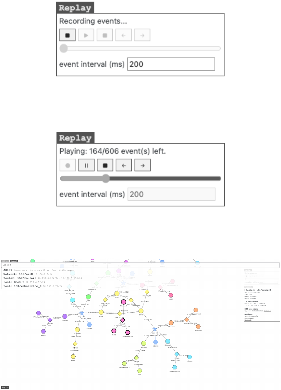
Figure 10: Replay controls: recording

Figure 11: Replay controls: playing

Figure 12: Search for nodes

Figure 13: Console window actions

7.1.6 Console windows

Each console window also has a few action buttons one can use. Figure 13 shows the buttons. From left

to right, the ﬁrst button allows one to close the console window. The console session will keep running

even after the window is closed; the reasons behind this decision will be detailed later in the backend

section. The second button allows one to minimize the window into the taskbar. The third button allows

one to “pop-out” the console window into a separate browser window. The fourth button allows one to

reload the console window; it is also possible sometimes that the WebSocket connection to the backend

breaks. A simple reload helps the connection to re-establish. One may also use the reload button to

restart the console session when they log out of the console. The last button allows one to toggle input

broadcast to the window. When multiple windows have input broadcast enabled, inputting to any of the

windows with broadcast enabled will duplicate the input into all other windows with broadcast enabled.

7.2 The backend

The backend of the web client hosts the frontend webpages, APIs, and WebSocket endpoints for the fron-

tend. It is also developed with Typescript and uses the dockerode and express framework. The former

provides an easy-to-use API wrapper for the docker socket; the latter is a web application framework.

The backend automatically discovers the docker control socket by looking at the DOCKER HOST envi-

ronment variable, and trying the default settings for docker if the environment is not set. The backend

is built from a few diﬀerent parts: the API server, the sniﬀer, the controller, and the session manager.

7.2.1 The API server

The API server provides RESTful APIs for the frontend to obtain information about nodes and networks

in the emulation. The node and network information are added by the docker compiler. Metadata like

the node’s name, display name and description of nodes, list of connected networks, and IP addresses in

the networks are all attached to the containers using labels. Set of labels attached to a node may look

like this:

Listing 20: Node labels

org.seedsecuritylabs.seedemu.meta.asn: "171"

org.seedsecuritylabs.seedemu.meta.nodename: "router0"

org.seedsecuritylabs.seedemu.meta.role: "Router"

org.seedsecuritylabs.seedemu.meta.net.0.name: "net0"

org.seedsecuritylabs.seedemu.meta.net.0.address: "10.171.0.254/24"

org.seedsecuritylabs.seedemu.meta.net.1.name: "ix105"

org.seedsecuritylabs.seedemu.meta.net.1.address: "10.105.0.171/24"

And, set of labels attach to a network may look like this:

Listing 21: Network labels

org.seedsecuritylabs.seedemu.meta.type: "global"

org.seedsecuritylabs.seedemu.meta.scope: "ix"

org.seedsecuritylabs.seedemu.meta.name: "ix101"

org.seedsecuritylabs.seedemu.meta.prefix: "10.101.0.0/24"

org.seedsecuritylabs.seedemu.meta.displayname: "San Jose-101"

The labels above are accessible through the docker control socket. The API server takes advantage of

these labels attached to each node to provide the metadata as a structured JSON object to the frontend.

The front end then uses this information to reconstruct the topology and draw the topology as a map.

The controller The controller provides some additional sets of APIs to the API server. The APIs

provided by the controller are more “dynamic” in the sense that they allow fetching information by

running commands on the node. The controller provides support for the BGP sessions and network

connection toggling feature. Those features require a piece of software, worker, to be running on the

node. The controller talks with the worker using the docker API by spawning a new instance of the

worker. The worker program is installed on all nodes by the docker compiler. Details about the worker

are in the next section.

The sniﬀer The sniﬀer feature allows one to perform packet capture on all nodes within the emulation.

It works by spawning new instances of tcpdump on all nodes, using the user-deﬁned ﬁlter. The sniﬀer

is the feature that enables the visualization of packet ﬂows on the front end. The idea behind the

visualization is, in fact, very simple. If a node receives a packet matching the given ﬁlter, the tcpdump

programs will print out new lines. When the front end sees these lines, it ﬂashes the corresponding

nodes. However, networks themselves are not nodes, and therefore, one cannot run tcpdump directly on

them. To be able to ﬂash both the network and the nodes, the frontend also collects MAC addresses of

all nodes in all networks. When the front end sees a packet from or to some MAC addresses belonging

to a known network, it ﬂashes the network.

The session manager The session manager manages console sessions for containers. The docker APIs

for spawning new programs inside containers do not have the ability to terminate the spawned programs

once they are started unless the program voluntarily exits. The session manager ensures that at most

one session is started for each container. If a session to a container already exists, it will return the old

session instead of creating new ones. It also monitors the sessions, so it knows to start a new session

upon request if the old one dies (generally caused by the user manually exiting the shell). Having only

one session for each node and keeping them running in the background also means if the front end exits,

one can re-open the front end and continue where they left oﬀ. It also prevents launching too many

sessions at the same time.

7.2.2 The worker

The worker program is a piece of software running on the node itself to allow the execution of arbitrary

commands by the backend. Features like disconnecting nodes from networks, listing BGP peers and their

status, and toggling BGP sessions are all based on the worker. The worker is required because when

running commands spawning in the shell session spawned by the docker, there will be no data boundaries.

The worker allows the backend to assign a task ID to every commands the backend requested and return

the execution result with the task ID and data boundaries. The execution is also done asynchronously.

The backend sends the command request out, registers a handler to listen for the response, and continues

to serve other requests.

One may argue that it is possible to spawn a new session for every command requested - it is,

however, very costly the spawn a new session and slows down the backend signiﬁcantly. It also means

some commands may not work well, as some of them were expecting to output to a pseudo-terminal,

which requires additional handlings.

8 Case study

8.1 Simple BGP setup

This section is going to explore the basics of emulation building with a simple emulation scenario. In

this section, three autonomous systems (AS150, AS151, and AS152) and one Internet exchange, IX100,

will be created. The three autonomous systems will each originate a single /24 preﬁx and peer with each

other at IX100. They will also host one single web server within their networks. The complete code for

this setup is available in listing 84 in the appendix.

8.1.1 Import and create required components

Listing 22: Importing components

from seedemu.layers import Base, Routing, Ebgp

from seedemu.services import WebService

from seedemu.compiler import Docker

from seedemu.core import Emulator, Binding, Filter

Listing 22 shows the code required to import the components in the simple BGP setup example. It

imported four layers:

• The Base layer provides the base of the emulation; it describes what hosts belong to what au-

tonomous system and how hosts are connected.

• The Routing layer acts as the base of the routing protocols. It does the following: (1) installing

BIRD Internet routing daemon on every host with the router role, (2) providing lower-level APIs

for manipulating BIRD’s FIB (forwarding information base) and adding new protocols, creating

pipes and other supporting features, and (3) setting up proper default route on non-router role

hosts to point to the ﬁrst router in the network.

• The Ebgp layer provides APIs for setting up External BGP peering.

• The WebService layer provides APIs for installing the nginx web server on hosts.

In order to compile the emulation into docker containers, the Docker compiler is imported. In order

to build the emulation, the core Emulator class is imported. And to facilitate virtual node binding for

the web services that will be hosted later, Binding and Filter is imported.

Listing 23: Initializing components

emu = Emulator()

base = Base()

routing = Routing()

ebgp = Ebgp()

web = WebService()

Once the classes are imported, initialize them as shown in the listing 23.

8.1.2 Create an Internet exchange

To enable BGP peerings, one can either create an Internet exchange or connect two routers in diﬀerent

autonomous systems using a cross-connect. In order to simplify the setup, this section will use an Internet

exchange to allow all autonomous systems to peer with each other.

Listing 24: Creating Internet exchange

base.createInternetExchange(100)

The Base::createInternetExchange function call creates a new Internet exchange. By default,

it creates a new global network name ixNNN with network preﬁx of 10.NNN.0.0/24, where NNN is

the ID of the Internet exchange. The exchange network can later be joined by router nodes us-

ing the Node::joinNetwork function call. One may optionally set the IX LAN preﬁx with the pre-

ﬁx parameter and the way it assigns IP addresses to nodes with the aac parameter when calling

createInternetExchange. Listing 24 shows how to create an Internet exchange with ID 100. With

the call, Internet exchange 100 is created. It creates the network ix100.

8.1.3 Create an autonomous system

Creating a new autonomous system in the emulator is a multistep process. It consists of the following

steps:

• Creating the autonomous system object.

• Creating an AS-internal network to connect router and hosts.

• Creating router.

• Creating host.

• Creating a virtual node and hosting service on it.

• Binding the service to the host.

Creating the autonomous system object. The very ﬁrst thing one would do to create new au-

tonomous systems is to invoke the createAutonomousSystem function of the base layer. Listing 25 shows

how one would call the method. The call returns an AutonomousSystem class instance, and it can be

used to further create hosts and networks in the autonomous system.

Listing 25: Creating autonomous system

as150 = base.createAutonomousSystem(150)

Creating an AS-internal network to connect router and hosts. The logical next step to take

when creating an autonomous system is to create an internal network for it. However, creating internal

networks is completely optional. One can create a stub autonomous system without any networks by

creating a single router and nothing more in the autonomous system. An example of such an autonomous

system can be an autonomous system that is used to perform BGP hijacks. To create a new internal

network, one would use the AutonomousSystem::createNetwork call.

The AutonomousSystem::createNetwork calls create a new local network (as opposed to the net-

works created by Base::createInternetExchange), which can only be joined by nodes from within the

autonomous system. Similar to the createInternetExchange call, the createNetwork call also auto-

matically assigns network preﬁxes; it uses 10.asn.id.0/24 by default, where the asn is the autonomous

system number, and id is a self-incrementing number. The createNetwork API call also accept prefix

and aac parameter for conﬁguring preﬁx and setting up auto address assignment.

By default, the network created by the call will have the direct attribute. This attribute instructs

the routing daemon (if it exists; i.e., if the Routing layer is added to the emulator.) to generate a route

matching the interface route in its routing information base. This route will then be re-distributed into

other routing protocols, like BGP, so that the BGP peers can learn the route and route traﬃc destinating

the network to the router. This behavior can be disabled by passing direct = False to the function

call.

Listing 26 shows how one can create a new internal network with the call. In the next few sections,

this network will be used for connecting the node hosting service and the edge router of the autonomous

system.

Listing 26: Creating an internal network

as150.createNetwork('net0')

Creating router. Once the internal network is created, one would need to create a router that con-

nects the internal network and the Internet (in this case, the “Internet” is IX100, where the other two

autonomous systems will be located.) For the router to route traﬃc between the Internet network and

the Internet exchange, it will need to connect to both of the networks.

One can create the router and have it join both networks with three API calls, chaining together in

one line, as shown in the listing 27. The AutonomousSystem::createRouter takes one parameter, the

name of the new node. The call creates a new router node with the given name. The call then returns

a Node object on success.

The Node::joinNetwork call connects a node to a network. It ﬁrst searches through the local

networks, then global networks. Internet exchanges, for example, are considered global networks. It can

also optionally take another parameter, address, to override the auto address assignment.

Listing 27: Creating a router

as150.createRouter('router0').joinNetwork('net0').joinNetwork('ix100')

Creating host. In order to host services within an autonomous system, one would need to create a

host node. Creating a host is not much diﬀerent from creating a router.

The AutonomousSystem::createHost API also takes one parameter, name, which is the name of

the host, and it will also return a Node instance on success. Listing 28 shows how one would create a

host named web and have it join the internal network with name net0.

Listing 28: Creating a host

as150.createHost('web').joinNetwork('net0')

Creating a virtual node and hosting service on it. Since now the router, host, and network have

been created, the logical next step to take is to install the service on the host node.

As a refresher, the SEEDEMU framework does not install services directly on a host node. To

install a service, one would ﬁrst install the service on a virtual node. Virtual nodes are not real nodes in

the sense that they are just an internal string in the Service interface for keeping track of changes to

make. Consider them as the “blueprint” of a physical node. They are decoupled from the physical node,

making reusing them much easier. Whenever one makes changes to the virtual nodes, the “blueprint”

is changed. Eventually, a virtual node needs to be mapped to a physical node using the binding system

to apply all the conﬁgurations and changes in the “blueprint” to the physical node. Physical nodes are

real nodes; they are the nodes created by the AutonomousSystem::createHost API.

In order to install web service on the node created before, one would need to ﬁrst use the Service::install

call. WebService class derives from the Service class, so it also has the install method. The install

method takes a virtual node name and install the service on that virtual node. Example of this is shown

in listing 29.

Listing 29: Installing service on virtual node

web.install('web150')

Binding the service to the host. To let the emulator knows where to bind the virtual node web150

created earlier to, one would add a Binding to the emulator. To bind a virtual node, one would need

Binding and Filter. Binding allows one to deﬁne binding for a given virtual node name, or a pattern of

virtual node names. Filter allows one to deﬁne some constraints on what physical nodes are considered

as binding candidates. Listing 30 shows how one can bind the virtual node web150 to the physical node

created earlier.

Listing 30: Creating binding

emu.addBinding(Binding('web150', filter = Filter(nodeName = 'web', asn = 150)))

Note that this is only one example of binding the virtual node to the physical node. Since there

is only one host node in AS150, the nodeName constraint can be safely omitted. Other constraints, like

network preﬁx and IP address, can be used to select candidates, which were discussed in the binding

section earlier.

At this point, an autonomous system with one internal network, one host node, one router, and

connected to IX100 is created. To create the rest of the autonomous systems, one can copy the code

above two more times and change the autonomous system number.

8.1.4 Set up BGP peerings

With all autonomous systems created, the next step is to set up BGP peerings, so they can exchange

routes with each other. Setting up BGP peering is done at the EBGP layer. Listing 31 shows how to

peer AS150, AS151, and AS152 at the Internet exchange IX100 with the route server.

Listing 31: Set up BGP peerings

ebgp.addRsPeer(100, 150)

ebgp.addRsPeer(100, 151)

ebgp.addRsPeer(100, 152)

Generally, there are two ways to set up BGP peerings within an Internet exchange. One is with

the multilateral peering agreement (MLPA) via a route server (RS). A route server peers with every

participant in the MLPA and send routes received from one peer to all other peers, without modifying

the AS PATH and NEXT HOP attribute (some outliers in the real world do modify the AS PATH attribute,

but it is the minority, and as long as the NEXT HOP attribute is not changed, the eﬀect of an RS is still the

same). This eﬀectively creates full mesh peering between all autonomous systems connected to the route

server. Another peering option is to set up a private one-to-one session. This example uses RS-based

MLPA peering.

8.1.5 Render and compile the emulation

The last step one would do to ﬁnish building the emulation is to render and compile the emulation. The

rendering process is where all the actual “emulation construction” happens. Software is added to the

nodes, routing tables and protocols are conﬁgured, and BGP peers are conﬁgured. Listing 32 shows how

to add layers to the emulator and render them.

Listing 32: Adding layers to emulator and render them

emu.addLayer(base)

emu.addLayer(routing)

emu.addLayer(ebgp)

emu.addLayer(web)

emu.render()

After all the layers are rendered, all the nodes and networks are created. They are still stored

using internal data structures (i.e., the core classes). The intermediate representations will need to be

“compiled” down to something the emulation platform, like docker, can understand. The name of such

a process is called compilation. The main focus of the framework is the docker compiler backend. As

such, this example will use the docker compiler.

Listing 33 shows how one would invoke the docker compiler. The docker compiler would generate

all the docker ﬁles inside the ./output folder. The docker compiler comes with a docker-compose

conﬁguration. To run the emulation, one can run docker-compose build && docker-compose up in

the output directory.

Listing 33: Using the docker compiler backend

emu.compile(Docker(), './output')

The detailed rendering and compilation logic is discussed in the rendering part in the design section.

8.2 Simple transit BGP setup

This example shows how one can create a transit provider in the emulator. AS150 will serve as a transit

for two other autonomous systems, AS151 and AS152, where AS151 will be located in IX100, and AS152

will be located in IX101. As most part of this example is the same as the simple peering example, the

detailed discussions will be omitted. Full code of this example is available in the appendix, listing 85.

8.2.1 Import and create required components

Two new layers are required for this example:

• IBGP layer: The IBGP layer setup full-mesh IBGP peering between all reachable internal routers.

• OSPF layer: The OSPF layer conﬁgure OSPF routing on all routers within the autonomous system.

8.2.2 Create a transit autonomous system

A transit autonomous system peers with other autonomous systems at multiple Internet exchange points,

pulling traﬃc from one place to another. In order to connect the BGP routers at these diﬀerent locations,

a transit AS typically has multiple internal networks.

Create AS150 and its internal networks To get started, AS150 needs to be created. Some internal

networks to support transiting traﬃc from one place to another should also be created. One can use

only one network to connect the two diﬀerent locations, but that is rarely the case in the real world.

Multiple internal networks are created to make the network look realistic. Listing 34 shows how one can

create the autonomous system and the internal networks.

Listing 34: Create AS150 and its internal networks

as150 = base.createAutonomousSystem(150)

as150.createNetwork('net0')

as150.createNetwork('net1')

as150.createNetwork('net2')

Create routers For AS150, four routers should be created to connect two sites. The two of them, R1

and R4, will be the provider edge routers that connect to the Internet exchange and provide services to

the other autonomous system. The other two of them, R2 and R3, will be regular provider routers that

connect to no customers and carry transit traﬃc between R1 and R4. This enables AS150 to transit

traﬃc between IX100 and IX101. Listing 35 shows how one can create the routers and connect them to

the networks.

Listing 35: Create and connect routers to networks

as150.createRouter('r1').joinNetwork('net0').joinNetwork('ix100')

as150.createRouter('r2').joinNetwork('net0').joinNetwork('net1')

as150.createRouter('r3').joinNetwork('net1').joinNetwork('net2')

as150.createRouter('r4').joinNetwork('net2').joinNetwork('ix101')

This example uses OSPF and IBGP as its internal routing option. IBGP and OSPF layers do

not need to be conﬁgured explicitly; they are by default enabled on all autonomous systems. One will

need to explicitly disable IBGP and OSPF for a network or autonomous systems should they want

to. The detailed behavior of the IBGP and OSPF layers is described in the design section. One can

alternatively use MPLS instead of the OSPF and IBGP internal routing option, which is detailed in the

next subsection.

8.2.3 Set up BGP peering

In this example, the peering between AS150 and AS151/AS152 is done over Internet exchange. It is

generally a less common practice to provide transit service over an Internet exchange; most providers

will require a direct connection to them to provide transit services. This example provides transit service

directly over Internet exchange to simplify the setup.

Listing 36: Conﬁgure BGP peers

ebgp.addPrivatePeering(100, 150, 151, abRelationship = PeerRelationship.Provider)

ebgp.addPrivatePeering(101, 150, 152, abRelationship = PeerRelationship.Provider)

Listing 36 shows how one would conﬁgure peering between AS150 and AS151/AS152. The line

ebgp.addPrivatePeering(100, 150, 151, abRelationship = Provider) conﬁgures peering between

AS150 and AS151 at IX100, where AS150 is AS151’s provider. Details about the peering relationship

are discussed in the design section.

8.2.4 Save the emulation for later use

This example will be used as the base of a few other examples later. To serialize the emulation as a

single binary ﬁle, one can use the Emulator::dump API. Listing 37 shows how one can invoke the API.

Listing 37: Dumping the emulation

emu.dump('base-component.bin')

The API call above dumps the emulation to a ﬁle named base-component.bin, which can be used

later. The emulation can also be rendered, compiled, and executed on its own. The process is the same

as in the last example. However, it should be noted that dump must happen before the render call.

8.3 Create a MPLS-based transit autonomous system

As an alternative to the IBGP and OSPF setup, transit providers may use MPLS as their internal

network option. With MPLS, non-edge routers do not need to carry the BGP routing table at all.

Non-edge routes only need to keep track of a small amount of MPLS labels, signiﬁcantly reducing the

resources needed on non-edge routes. MPLS also oﬀers the capability to traﬃc engineering, where the

traﬃc does not follow the best path elected by IGP but rather route traﬃc around traﬃc hot-spots

that satisﬁes some given conditions like bandwidth or latency. However, note that no traﬃc engineering

support is added in the SEEDEMU framework. Details about how the MPLS layer works are discussed

in the design section.

The full code for this example is at appendix, listing 86.

8.3.1 Host system support

MPLS requires support from the Linux kernel; for this example to work properly, one will need to load

the MPLS kernel module on the emulator host with the following command, as root:

Listing 38: Loading the MPLS module

# modprobe mpls_router

8.3.2 Import and create required components

Only one new layer, the MPLS layer, is required for this example. Unlike IBGP and OSPF layers, MPLS

is not enabled for an autonomous system unless explicitly conﬁgured. MPLS and the IBGP/OSPF setup

are also mutually exclusive. One cannot use both setups for the same autonomous system. One can,

however, use the same setup for diﬀerent autonomous systems in the same emulation. The MPLS layer

automatically disables OSPF and IBGP for MPLS-enabled autonomous systems.

8.3.3 Create a transit autonomous system

Conﬁgure MPLS Unlike OSPF and IBGP, MPLS needs to be explicitly enabled for an autonomous

system. This can be done with the Mpls::enableOn API:

Listing 39: Enabling MPLS on AS150

mpls.enableOn(150)

Here, only r1 and r4 are edge routers; thus, IBGP session will only be set up between them. r2

and r3 will only participate in OSPF and LDP. The topology looks like this:

Listing 40: MPLS topology

| AS150's MPLS backbone |

| ____________ ibgp ___________ |

| / \ |

as151 -|- as150_r1 -- as150_r2 -- as150_r3 -- as150_r4 -|- as152

| |

Since r2 and r3 don’t carry the tables from AS151 and AS152, traceroute will look like this:

Listing 41: Traceroute result

HOST: 0e58e675b98b Loss% Snt Last Avg Best Wrst StDev

1.|-- 10.152.0.254 0.0% 10 0.1 0.1 0.1 0.1 0.0

2.|-- 10.101.0.150 0.0% 10 0.1 0.1 0.1 0.2 0.0

3.|-- ??? 100.0 10 0.0 0.0 0.0 0.0 0.0

4.|-- ??? 100.0 10 0.0 0.0 0.0 0.0 0.0

5.|-- 10.150.0.254 0.0% 10 0.1 0.1 0.1 0.2 0.0

6.|-- 10.100.0.151 0.0% 10 0.3 0.2 0.1 0.3 0.1

7.|-- 10.151.0.71 0.0% 10 0.2 0.2 0.1 0.3 0.0

The two missing hops are r2 and r3. One can also validate that the network is indeed running on

MPLS by tcpdump:

Listing 42: tcpdump result

root@d5d8ad0d6d48 / # tcpdump -i net1 -n mpls

tcpdump: verbose output suppressed, use -v or -vv for full protocol decode

listening on net1, link-type EN10MB (Ethernet), capture size 262144 bytes

19:39:33.831880 MPLS (label 21, exp 0, [S], ttl 61) IP 10.152.0.71 > 10.151.0.71: ICMP echo

request, id 123, seq 1, length 64

19:39:33.832051 MPLS (label 19, exp 0, [S], ttl 61) IP 10.151.0.71 > 10.152.0.71: ICMP echo

reply, id 123, seq 1, length 64

19:39:34.877246 MPLS (label 21, exp 0, [S], ttl 61) IP 10.152.0.71 > 10.151.0.71: ICMP echo

request, id 123, seq 2, length 64

19:39:34.877314 MPLS (label 19, exp 0, [S], ttl 61) IP 10.151.0.71 > 10.152.0.71: ICMP echo

reply, id 123, seq 2, length 64

4 packets captured

4 packets received by filter

0 packets dropped by kernel

8.4 Exploring emulator features with the simple transit BGP setup

One major feature of the SEEDEMU framework is the ability to share and reuse emulations. The

following subsections will show how to reuse the base layers built in the simple transit BGP setup for

diﬀerent emulation scenarios.

8.4.1 Allow real-world access to the emulation

The ability to connect to the inside of the emulation from the outside world and connect to real-world

hosts from within the emulation is an integral part of the SEEDEMU framework. In this case study,

a VPN server is conﬁgured to allow outside hosts to connect to the emulated network. A real-world

autonomous system is introduced into the emulation to route traﬃc outside the emulation. A real-world

autonomous system will collect the real network preﬁxes from the real Internet and announce them inside

the emulator. Packets reaching this autonomous system will exit the emulator and be routed to the real

destination. Responses from the outside will return to this real-world autonomous system and be routed

to the ﬁnal destination in the emulator.

Enable remote access Most of this part is the same as the transit BGP setup, with the only diﬀerence

being:

Listing 43: Import OpenVPN remote access provider

ovpn = OpenVpnRemoteAccessProvider()

For details about the OpenVPN remote access provider, check the feature section. Listing 43 creates

the remote access provider. To use it, one will have to pass it to the enableRemoteAccess API of the

network object. For example, to allow remote access to network net0 of AS150, one can do:

Listing 44: Use OpenVPN remote access provider

as151.createNetwork('net0').enableRemoteAccess(ovpn)

The Network::enableRemoteAccess call enables remote access to a network. The API takes only

one parameter, the remote access provider. Details on how to access the network with OpenVPN remote

access enabled are in the feature section.

Create real-world autonomous system A real-world autonomous system is just a regular au-

tonomous system with a real-world router in it. The ﬁrst step for creating a real-world autonomous

system is to create an autonomous system object:

Listing 45: Create the autonomous system

as11872 = base.createAutonomousSystem(11872)

Once the autonomous system is created, one can start creating the router for routing traﬃc to the

real world. Instead of the createRouter API, one would use the createRealWorldRouter for this task.

Listing 46: Create the real-world router

rw = as11872.createRealWorldRouter('rw')

Listing 46 shows how one can create a real-world router in AS11872 with the name rw. Details

about the createRealWorldRouter are in the feature section. This router will now fetch the preﬁxes

announced by AS11872 on the real Internet and announce those preﬁxes into the emulation. The next

step would be connecting the router to an Internet exchange so that the BGP routes can propagate in

the emulator. To join an exchange, one will need to override the auto address assignment manually. By

default, the address in the Internet exchange is assigned using the autonomous system number as the

oﬀset. Since the oﬀset 11,872 is out of the /24 range, the address needs to be assigned manually:

Listing 47: Joining the exchange

as11872.createRealWorldRouter('rw').joinNetwork('ix101', '10.101.0.118')

Other steps, like conﬁguring BGP peers, are similar to the BGP transit case, and therefore not

repeat here. Complete code for this case is in appendix, listing 87.

8.4.2 Customizing the visualization

One may change the name shown under the nodes and networks on the web UI programmatically. One

can also attach a text description to nodes and networks, which will be shown when the node is selected.

Each object (nodes and network) already has a name, but one may want to change them to something

more meaningful.

It is possible to set display names and descriptions of physical nodes (routers and hosts), virtual

nodes, and networks (local and Internet exchange). Setting display names and descriptions of virtual

nodes uses the virtual physical node feature, where a “fake” physical node is created for the given virtual

node name. Settings on the “fake” physical node are copied to the real physical node upon binding.

Listing 48 shows how one may set display names and descriptions.

Listing 48: Setting node/network display name and description

# set name/description for physical nodes

as151 = base.getAutonomousSystem(151)

as151.getRouter('router0').setDisplayName('AS151 Core Router')

as151.getRouter('router0').setDescription('The core router of AS151')

as151.getHost('web').setDisplayName('example.com')

as151.getNetwork('net0').setDisplayName('AS151 Main Network')

# set name/description for virtual node

as150.getVirtualNode('web150').setDisplayName('as150.net')

# set name/description for IX network

ix100_lan = base.getInternetExchange(100).getPeeringLan()

ix100_lan.setDisplayName('Seattle')

ix100_lan.setDescription('The Seattle Internet Exchange')

ix101_lan = base.getInternetExchange(101).getPeeringLan()

ix101_lan.setDisplayName('New York')

8.4.3 Components and emulator merging

One major feature of the SEEDEMU framework is the ability to re-use previously built emulations.

Recall that at listing 37, the emulation was saved to a ﬁle named base-component.bin. This section

covers how one may load and work with the dumped emulation.

Create a new emulator and load the dump ﬁle The ﬁrst step to load any existing emulation is

to create a new emulator and invoke the load method on the dumped ﬁle:

Listing 49: Load dumped emulation

emu = Emulator()

emu.load('../01-transit-as/base-component.bin')

Once the emulation is loaded, one may make changes to it. To make changes to existing layers, one

can use the getLayer call like this:

Listing 50: Retrieving layers from emulator

base: Base = emu.getLayer('Base')

ebgp: Ebgp = emu.getLayer('Ebgp')

The layer retried from the call can be interacted with normally. Listing 51 shows how one can make

changes.

Listing 51: Interactive with the layers

# get an autonomous system from base layer, and a create new host.

as151 = base.getAutonomousSystem(151)

as151.createHost('web-2').joinNetwork('net0')

# add new peerings

ebgp.addPrivatePeering(100, 150, 153, abRelationship = PeerRelationship.Provider)

ebgp.addPrivatePeering(100, 151, 153, abRelationship = PeerRelationship.Peer)

Merging emulations It is also to merge two emulator objects. The two emulators can come from

pre-built emulations (i.e., loaded using the load API) or be newly created using code. Each emulation

can have its own autonomous systems, Internet exchanges, networks, virtual nodes, and more. The

SEEDEMU framework will try to merge them automatically.

Generally, the SEEDEMU framework can automatically merge:

• Emulations that have no common layers at all. For example, if one emulation has the base layer,

routing layer, OSPF layer, and BGP layer, and the other one has DNS service layer, web ser-

vice layer, and the Ethereum layer. SEEDEMU framework can merge the two emulations fully

automatically. Users may still need to create virtual node bindings to allow the services to be

installed.

• Emulations that have no common autonomous systems at all. For example, if one emulation has

AS150 and IX100, and the other emulation has AS151 and, also, IX100. SEEDEMU framework

can merge the two emulations fully automatically. However, to “connect” the emulation, one may

need to conﬁgure the EBGP layer to have AS150 and AS151 peer with each other in the new

emulation. Or, if they have both already conﬁgured to peer with the route server, there is no need

to manually add peerings.

• Emulations with no overlapping virtual nodes at all. SEEDEMU can also handle merging most

of the service layers automatically, as long as there are no conﬂicting virtual node names. When

merging, one can optionally set a preﬁx to be prepended to every virtual node name of one of

the targets to prevent conﬂicts. Some services, like DNS services, may fail to merge if there are

conﬂicting records (for example, if aaa.example.com is a record in one emulator but is hosted as

a zone in the other emulator).

The next few sections will show how one may use the merging feature extensively to enable many

diﬀerent re-use use cases.

Listing 52: Merge emulations

emuA = Emulator()

emuA.load('base-component.bin')

emuB = Emulator()

emuB.load('dns-infrastructure.bin')

emuC = Emulator()

emuC.load('blockchain.bin')

emu = emuA.merge(emuB).merge(emuC, mergers = DEFAULT_MERGERS, vnodePrefix = 'eth-')

Listing 52 shows how one may merge the emulations. The merge call takes three parameters.

The ﬁrst is the other emulator. This emulator will be merged with the current emulator. The next

two parameters are optional. The ﬁrst one is a list of mergers. The Merger class handles merging of

individual layers if there are two layers of the same type in two emulators. The third option is the virtual

node preﬁx. The preﬁx will be prepended to all virtual nodes in the other emulator.

In listing 52, emulator A is ﬁrst merged with emulator B. No mergers have been used. This assumes

there are no common layers in A and B. Then, the resulting emulator is merged with emulator C. This

time, DEFAULT MERGERS is used as the mergers. The DEFAULT MERGERS constant is a constant list that

contains all the default merger implementations included with the SEEDEMU framework. It also adds

preﬁx eth- to all virtual nodes from emulator C. The ﬁnal result is then stored in emu.

8.5 Complex BGP setup

The next case study sets up a more comprehensive example. It creates six Internet exchanges, ﬁve

transits, and 12 stubs. One of the autonomous systems (AS11872) is a real-world autonomous system,

which announces the real-work network preﬁxes to the emulator. Packets to these preﬁxes will be routed

out to the real Internet. Another autonomous system (AS152) allows machines from the outside to join

the emulation (via VPN), so one can interact with the emulated hosts inside the emulator using a real

host.

8.5.1 The helper tools

In order to speed up the creation of the emulation, the SEEDEMU framework includes some helper tools

to allow the fast creation of commonly seen topologies.

makeTransitAs The makeTransitAs tool allows one to create a transit provider in the base layer

that takes four parameters. The ﬁrst parameter is the reference to the Base layer object. The second

parameter is the autonomous system number to use for the newly created provider. The third parameter

is a list of Internet exchange IDs to create routers for this provider. The last parameter is a list of

tuples, where each tuple contains two Internet exchange IDs. The makeTransitAs tool will create an

internal link between the two routers in the given Internet exchange. IBGP and OSPF will run across

all connected links, eﬀectively turning the autonomous system into a transit provider.

makeStubAs The makeStubAs tool allows one to create a stub autonomous system. A stub au-

tonomous system does not provide transit to other autonomous systems. The makeStubAs tool takes ﬁve

parameters:

• The ﬁrst parameter is the reference to the emulator object. Unlike makeTransitAs, the makeStubAs

tool can also create host nodes with services on them and therefore needs to create new bindings

in the emulator.

• The second parameter is the reference to the Base layer object to create nodes and networks in.

• The third parameter is the autonomous system number to use for the newly created stub au-

tonomous system.

• The fourth parameter is the ID of the Internet exchange to join with the stub.

• The last option is a list of services to host in the autonomous system’s network. The element of

the list can either be a reference to a Service layer object or None. For each element in the list,

one host node will be created. If the element is a Service layer object reference, one new server

will be installed on a virtual node, and the virtual node will be bound to the newly created host

node. If the element is None, a host node with no service is created.

The two helpers allow one to quickly create large transits and host various services.

8.5.2 Building the topology

Creating transit The following example creates a transit, AS2, which has a presence at three Internet

exchanges (ix100, ix101, and ix102). It also creates two internal networks to connect the three BGP

routers of this transit:

Listing 53: Create transit

Makers.makeTransitAs(base, 2, [100, 101, 102], [(100, 101), (101, 102)])

One can use multiple calls to makeTransitAs to create multiple transits in the emulator.

Creating stub The following example creates a stub, AS153, which has a presence at ix101. Three

hosts will be created for this stub, one running a web service, and the other two not running any service.

Listing 54: Create stub

Makers.makeStubAs(emu, base, 153, 101, [web, None, None])

Real-world integration The example creates a real-world autonomous system AS11872, which is

Syracuse University’s autonomous system. It will collect the network preﬁxes announced by this au-

tonomous system in the real world and announce them inside the emulator. Packets (from inside the

emulator) going to these networks will be routed to this autonomous system and forwarded to the real

world. Returning packets will come back from the outside, enter the emulator at this autonomous system,

and be routed to their ﬁnal destination inside the emulator.

Listing 55: Create real-world AS

as11872 = base.createAutonomousSystem(11872)

as11872.createRealWorldRouter('rw').joinNetwork('ix102', '10.102.0.118')

Real-world access The autonomous system AS152 is conﬁgured to allow real-world access. This

means machines from outside the emulator can VPN into AS152’s network, and becomes a node of the

emulator. This allows outside real-world machines to participate in the emulation.

Listing 56: Allow remote access from the real world

as152 = base.getAutonomousSystem(152)

as152.getNetwork('net0').enableRemoteAccess(ovpn)

Other details, like repetitive calls to the helpers and codes that have been demonstrated in earlier

sections, are skipped. The complete code for this example is available at appendix, listing 88.

8.6 Exploring emulator features on the complex BGP setup

The next few sections will deploy diﬀerent services on the same underlying topology built from the

complex BGP setup example (the last section).

8.6.1 BGP hijacks

BGP hijack generally can be performed without making modiﬁcations to the BGP setup at all. However,

to simplify the setup, this example will create a dedicated autonomous system for performing the hijack.

A new autonomous system, AS199, is created to be the attacker. The attacker is connected to IX105,

and using AS2 as their upstream.

Listing 57: Add attacker to the complex BGP setup

#!/usr/bin/env python3

# encoding: utf-8

from seedemu.core import Emulator

from seedemu.compiler import Docker

from seedemu.layers import Base, Ebgp, PeerRelationship

emu = Emulator()

# Load the pre-built component

emu.load('../B00-mini-internet/base-component.bin')

base: Base = emu.getLayer('Base')

ebgp: Ebgp = emu.getLayer('Ebgp')

# Create a new AS as the BGP attacker

as199 = base.createAutonomousSystem(199)

as199.createNetwork('net0')

as199.createHost('host-0').joinNetwork('net0')

# Attach it to ix-105 and peer with AS-2

as199.createRouter('router0').joinNetwork('net0').joinNetwork('ix105')

ebgp.addPrivatePeerings(105, [2], [199], PeerRelationship.Provider)

# Render and compiler

emu.render()

emu.compile(Docker(), './output')

Listing 57 shows the full code for the example. It ﬁrst loads the dump from the complex BGP setup

example and adds the attacker autonomous system.

Say if one wants to hijack AS153’s network, 10.153.0.0/24, they can announce two smaller preﬁxes

10.153.0.0/25 and 10.153.0.128/25. Any IP address inside 10.153.0.0/24 will match two IP preﬁxes,

one announced by the attacker and the other one announced by AS153, but the one announced by the

attacker has a longer match (25 bits, compared to the 24 bits from AS-153), the attacker’s preﬁx will be

selected by all the BGP routers on the Internet.

It should be noted that if the attacker announces /24, the hijack may still work in some parts of the

network, given that the attacker’s route is preferred. Also, in the real world, the longest preﬁx allowed

in the DFZ is /24. So, realistically, a /25 preﬁx will not be accepted by any of the peers, and therefore

hijacking with /25 preﬁxes will not work (but one can still hijack a /23 with two /24s with the same

principle). Max preﬁx length is not enforced by the EBGP layer.

There are also techniques, like RPKI [24], to cryptographically enforce route origin validation. RPKI

is a PKI for routing preﬁxes. Only resource holder has access to the PKI, and the holders can issue

certiﬁcates to authorize announcements. RPKI allows one to deﬁne the maximum preﬁx length and

the source autonomous system for a preﬁx. If a network enforces RPKI and sees a mismatch source

autonomous system or preﬁx length, it will discard the route. However, this still does not solve the

hijack issues, as the attacker can also forge autonomous system numbers. The max-length may limit the

impact to some extent, but the attacker can still archive hijack.

BIRD conﬁguration To actually perform the hijack, one would ﬁrst start the emulator. Once the

emulation is started, navigate to AS199’s router, and edit /etc/bird/bird.conf, BIRD’s conﬁguration

ﬁle.

Listing 58: BIRD conﬁguration for hijacking

protocol static hijacks {

ipv4 {

table t_bgp;

};

route 10.153.0.0/25 blackhole { bgp_large_community.add(LOCAL_COMM); };

route 10.153.0.128/25 blackhole { bgp_large_community.add(LOCAL_COMM); };

}

Listing 58 shows how one may hijack AS153’s preﬁx. The snippet above should be added to the

end of BIRD’s conﬁguration ﬁle. It adds two static routes to BGP’s routing table, t bgp. Community

LOCAL COMM is attached to the routes so that the routes will be exported to AS199’s upstream. Once the

conﬁguration is saved, tell BIRD to reload its conﬁguration using the command birdc configure, and

AS153’s preﬁx should now be hijacked.

Testing To test if the hijack works, pick any hosts on the emulated Internet (other than hosts from

AS199 or AS153), and ping one of the AS153’s hosts. If the hijack worked, there would be no response.

To see where the packets go, one can start the web UI and set the ﬁlter to icmp. One will see that all

the ping packets are rerouted to AS199. Next, to mitigate the damage, one can ﬁnd AS199’s router on

the web UI, select the router node, and disable its BGP peer. Traﬃc should be routed back to AS153

once the session at AS199 is disabled, and the ping program should also be able to see replies now.

Hijack the “real world” It will be more fun to launch such an attack on the real autonomous system,

but without doing real damages to the real world. Remember that the complex BGP setup includes one

real-world autonomous system, AS11872, in the emulation. AS11872 is announcing the real-world preﬁx

of AS11872 and routing traﬃc to the real AS11872. The emulator eﬀectively becomes a shadow Internet.

One can easily hijack AS11872 inside the emulator and experience the eﬀect of the hijack if it were to

happen in the real world, without aﬀecting the real-world AS11872.

8.6.2 Deploying DNS

This section covers how one may build a portable DNS infrastructure and deploy the infrastructure on

the complex BGP setup example.

Building the infrastructure At its core, the DNS infrastructure is merely a set of DNS servers, where

the root servers point to the TLD servers, and the TLD servers point to individual domain servers. To

begin, install the root servers onto the virtual nodes, and host the root zone (.) on them.

Listing 59: Creating root servers

dns.install('a-root-server').addZone('.').setMaster() # master server

dns.install('b-root-server').addZone('.') # slave server

# ...

dns.install('a-com-server').addZone('com.').setMaster()

dns.install('b-com-server').addZone('com.')

# ...

dns.install('ns-twitter-com').addZone('twitter.com.')

Each of the call in listing 59 creates a virtual node. Then, a zone is conﬁgured on the virtual node.

It is possible to have multiple servers hosting the same zone. In such a case, setMaster() should be

invoked to set one of the servers as the master server of the zone. It should be noted that, since the goal

is to create a portable DNS infrastructure, there should not be binding speciﬁed for these virtual nodes

(and not possible to, since there is no base layer in this emulation at all). Binding will be conﬁgured

when one wants to use this with another emulation that has a base layer.

One may also want to pre-deﬁned some records in the zone. This can be done by ﬁrst retrieving the

zone with the getZone API, then invoke addRecord method on the zone object, as shown in the listing

60. As will be soon shown, it is also possible to add A record that points to IP addresses of virtual nodes.

Listing 60: Adding records

dns.getZone('twitter.com.').addRecord('@ A 10.0.0.1').addRecord('www A 10.0.0.2')

Dumping the DNS infrastructure Like any other emulation, the DNS infrastructure can be saved

as a ﬁle:

Listing 61: Dumping the infrastructure

emu.addLayer(dns)

emu.dump('dns-component.bin')

Full code for the DNS infrastructure setup is in the appendix, listing 89.

Load and merge with the complex BGP setup To use the infrastructure, it needs to deploy on

another emulation that has a base layer to function. This example uses the complex BGP set up as the

base. The overall steps are:

• Load the two previously built emulations. Merge them into a new one.

• Create bindings for the DNS servers. One may create one catch-all binding with no ﬁlter to have

all DNS servers installed onto random physical nodes, conﬁgure bindings for every single node, or

anything in between.

• Create a DNS caching server. Clients do not perform recursive DNS lookups themselves. DNS

caching server, or recursive DNS server, must be conﬁgured inside the emulator for clients to use.

To load and merge the emulations, one may do this:

Listing 62: Merging emulations

emuA.load('../B00-mini-internet/base-component.bin')

emuB.load('../B01-dns-component/dns-component.bin')

emu = emuA.merge(emuB, DEFAULT_MERGERS)

Next, bind the DNS nodes:

Listing 63: Binding DNS nodes

# bind root servers randomly in AS171

emu.addBinding(Binding('.*-root-server', filter=Filter(asn=171)))

# bind com servers randomly in AS151, net on 152, edu on 153, and cn on 154

emu.addBinding(Binding('.*-com-server', filter=Filter(asn=151)))

emu.addBinding(Binding('.*-net-server', filter=Filter(asn=152)))

emu.addBinding(Binding('.*-edu-server', filter=Filter(asn=153)))

emu.addBinding(Binding('.*-cn-server', filter=Filter(asn=154)))

# for the domain servers, bind them randomly in any AS

emu.addBinding(Binding('ns-.*'))

Listing 63 only shows one way to bind the DNS servers. If one does not know the name of vir-

tual nodes or does not care about where the servers will end up, then they can just use one binding

Binding(’.*’) to cover everything. More details about the binding system are in the design section.

Next, create the recursive DNS and bind them somewhere:

Listing 64: Binding DNS nodes

ldns = DomainNameCachingService()

ldns.install('global-dns-1')

ldns.install('global-dns-2')

emu.addBinding(Binding('global-dns-1', filter = Filter(ip = '10.152.0.53')), action =

Action.NEW)

emu.addBinding(Binding('global-dns-2', filter = Filter(ip = '10.153.0.53')), action =

Action.NEW)

Listing 64 uses the NEW action of the binding system. As a recap, the NEW action tries to create

node matching to ﬁlter rule instead of looking for nodes that match the ﬁlter. The action NEW is a good

ﬁt when one wants to add something new to the existing emulation. While they can manually retrieve

the base layer, get the autonomous system object, create a host manually, then create binding for the

host to install service, the NEW action massively simpliﬁes the process. The ip option is used here since

settings name servers for nodes require one to provide the IP address of the name server.

Last, conﬁgure nodes to use the recursive DNS created in the last step:

Listing 65: Set name servers

base.getAutonomousSystem(170).setNameServers(['10.152.0.53'])

base.setNameServers(['10.153.0.53'])

One may set name servers for a single host, all hosts within an autonomous system, or all nodes

within the emulation. Listing 65 shows how one may set the name server at the autonomous system

level and at the emulation level. Settings at the autonomous system level override the settings at the

emulation level.

Once all the steps are done, add the local DNS layer to the emulator, then render and compile the

emulation. The resulting emulation will have the same topology as the complex BGP setup but is now

complete with the DNS infrastructure. The complete code for this example is in the appendix, listing

90.

8.6.3 Deploying anycast

The IP anycast technology allows multiple computers on the Internet to have the same IP address. When

another machine sends a packet to this IP address, one of the computers will get the packet. Exactly

which one will get the packet depends on BGP routing. IP anycast is naturally supported by BGP.

One of the well-known applications of IP anycast is the DNS root servers. Some DNS root servers,

such as the F server, have multiple machines geographically located in many diﬀerent places around the

world, but they have the same IP address. For example, all the F servers have the same IP address

192.5.5.241. When a DNS client sends a request to this IP address, one of the F servers will get the

request.

Load the base emulator This example will again be based on the complex BGP setup. To get

started, the emulation needs to be ﬁrst loaded:

Listing 66: Loading previously built emulation

emu.load('../B00-mini-internet/base-component.bin')

base: Base = emu.getLayer('Base')

ebgp: Ebgp = emu.getLayer('Ebgp')

This example will be adding a new autonomous system to perform the anycast. Listing 66 therefore

retrieves the EBGP and the base layer from the loaded emulation.

Create autonomous system Next, create the new autonomous system that will be used for the

anycast setup. Create two networks with the same preﬁx, and create two hosts in those networks with

the same IP address:

Listing 67: Creating the anycast AS ans hosts

as180 = base.createAutonomousSystem(180)

as180.createNetwork('net0', '10.180.0.0/24')

as180.createNetwork('net1', '10.180.0.0/24')

as180.createHost('host0').joinNetwork('net0', address = '10.180.0.100')

as180.createHost('host1').joinNetwork('net1', address = '10.180.0.100')

Create two hosts with the same IP Router for the two networks will be created in the next step.

This setup intentionally creates two disjoint parts, meaning there will be no link between the two routers

to connect the two networks.

Listing 68: Creating the routers

as180.createRouter('router0').joinNetwork('net0').joinNetwork('ix100')

ebgp.addPrivatePeerings(100, [3, 4], [180], PeerRelationship.Provider)

as180.createRouter('router1').joinNetwork('net1').joinNetwork('ix105')

ebgp.addPrivatePeerings(105, [2, 3], [180], PeerRelationship.Provider)

Listing 68 creates two routers for the two networks created in the last step. There is no link between

the two routers, but both routers connect to an Internet exchange and use two diﬀerent ISPs in the

exchanges as providers.

At this point, the setup is complete. Render, compile, and start the emulation. Pinging the anycast

host 10.180.0.100 should send the traﬃc to one of the hosts. Setting ﬁlter to icmp on the web UI

should allow one to visualize the packet ﬂow in the emulator. Trying from diﬀerent source hosts should

result in diﬀerent anycast hosts. Complete code for this example is available in appendix, listing 91.

8.7 Developing a new layer

To add new functionality into the emulator that works with the entire emulation as a whole, one can

create a new layer. Generally, if one is creating something that only works with a single node, like a

service (like a web-based app), they should create a service layer, which is discussed in the next section

instead.

To create a new layer, one will need to implement the Layer interface. The Layer interface is actually

fairly simple. It only has two methods.

8.7.1 Implementing the Layer interface

Layer::getName All layers must implement the getName method. This method takes no input and

returns a string indicating the name of this layer. The name of the layer must be unique. The name of

the layer will be used as the identiﬁer for the layer object in the emulator.

Layer::render All layers must implement the Layer::Render method. This method takes one param-

eter, the reference to the Emulator class instance, as input. It does not need to return anything. Layers

should make changes to the objects in the emulation here. In the render stage, layers can safely assume

that no further API calls will be made on the Layer class itself. An example of this is the DNS service

layer. The DNS layer will start collecting nameservers for zones, ﬁnalize glue records, convert the internal

tree structure to zone ﬁles, etc. No more changes can be made to the layer - meaning no new domains

can be added, no more name servers can be added.

8.7.2 Implementing the Conﬁgurable interface

The Layer interface is derived from the Conﬁgurable interface. The Conﬁgurable class has only one

method:

Conﬁgurable::conﬁgure Layers may optionally implement the Conﬁgurable::conﬁgure method. This

method takes one parameter, the reference to the Emulator class instance, as input. It does not need

to return anything. A default implementation of Conﬁgurable::conﬁgure is included in the Conﬁgurable

class - it just returns when called. Layers can make changes to the objects, or even another layer, in the

emulation here.

Unlike the render stage, the layer should allow future changes to the layer, as other layers may make

changes during their conﬁguration stage. An example of this is, again, the DNS service layer. Layers

like ReverseDomainNameService collect IP addresses in the emulator and assign reverse hostnames to

them by creating a new in-addr.arpa. zone in the DNS layer.

In the conﬁguration stage, a layer should register objects that may be useful to other layers in the

emulator. An example of this is the base layers. Node and Network objects are, in fact, registered in the

emulator in the conﬁguration stage by the base layer.

A Node object represents a network device in the emulator. It can be a server, a router, a user

machine, or any other device connected to the network. A Network object represents a network in the

emulator. It can be a private local network within an autonomous system or a public global network like

an Internet exchange.

8.7.3 Working with the global object registry

To access another object in the emulator, one will use the Registry. Consider Registry as a database

of objects in the emulator. Nodes, networks, and even other layers are registered in the Registry. To

retrieve the Registry, use Emulator::getRegistry. The Emulator object is passed to layers in both

render and conﬁguration stages.

To retrieve an object from the Registry, one will need to know the scope, type, and name of the

object. The scope is usually the name of the owner of the object. For private Node and Network, it is

usually their autonomous system number. Type, as the name suggested, speciﬁes the type of the object.

Examples are network for Network, hnode for Node with host role, and rnode for Node with router role.

The name also deﬁnes the name of the object.

For example, to get a router node with name router0 from AS150, one can do:

Listing 69: Getting objects from the global registry

r0_150: Router = emulator.getRegistry().get('150', 'rnode', 'router0')

Example of locations of some other objects in the emulator (in the format of scope/type/name):

• AS150’s host node with name web server: 150/hnode/web server.

• IX100’s peering LAN: ix/net/ix100.

• IX100’s router server node: ix/rs/ix100.

• The Base layer: seedemu/layer/Base.

To test if an object exist, use has:

Listing 70: Testing object existent in the global registry

if registry.has('150', 'rnode', 'router0'):

# do something...

To iterate over all objects, use getAll:

Listing 71: Iterating through all objects in the global registry

for ((scope, type, name), obj) in registry.getAll().items():

# do something...

To iterate over all objects of a type in a scope, use getByType:

Listing 72: Iterating through all objects of some type in the global registry

for router in registry.getByType('150', 'rnode'):

# do something...

To register an object, use register:

Listing 73: Registering new object in the global registry

registry.register('some_scope', 'some_type', 'some_name', some_object)

For an object to be registrable, it must implement the Registrable interface.

8.7.4 Working with other layers

As mentioned earlier, layers may access each other and make changes to each other. While having the

two-stage process helps with making changes in order, sometimes it may be necessary to have some layers

to be conﬁgured before or after another layer. The most obvious example of this is the base layer. The

base layer must be conﬁgured before all other layers. Otherwise, they will not be able to retrieve the

Node and Network objects from the Registry.

A layer can require itself to be rendered before or after another layer or ask the emulator to error out

when another layer does not exist. This mechanism is called layer dependency. To add a dependency,

layer can call Layer::addDependency.

The addDependency API takes three parameters:

• layerName: string, name of the layer to target.

• reverse: A boolean, when True, this addDependency creates a reverse dependency. Regular

dependency requires the target layer to be rendered/conﬁgured before the current layer, while a

reverse dependency requires the current layer to be rendered/conﬁgured before the target layer.

• optional: A boolean, when True, the emulator will continue rendering even if the target layer

does not exist in the emulation.

8.7.5 Working with merging

Merging is an essential feature of the emulator. It enables the re-use of existing layers in another

emulation. One can build and public a full DNS infrastructure without the base layer. Other users can

then merge the DNS infrastructure with their own emulation with the base layer without re-building the

DNS infrastructure themselves.

During merging, the same layer may exist in both emulators. A Merger class needs to be imple-

mented to handle the merging. The Merger interface are as follows:

Merger::getName The getName call takes no parameter and should return the name of the merger.

This should be a unique identiﬁer of the merger.

Merger::getTargetType The getTargetType call takes no parameter and should return the name

of type that this merger targets. For example, a merger that targets the Base layer should return a

BaseLayer object here.

Merger::doMerge The doMerge call takes two parameters. Call them objectA and objectB. When

user performs a merge by calling newEmulator = emulatorA.merge(emulatorB), objectA will be the

object from emulatorA, and objectB will be the object from emulatorB. The call should return a new,

merged object of the same type with the objectA and objectB.

8.8 Developing a new service

Services are special kinds of layers. One way to diﬀerentiate the regular and services layers is how they

make changes to the emulation. A regular Layer changes the entire emulation (like BGP, which conﬁgure

peeing across multiple diﬀerent autonomous systems, exchanges, and routers). In contrast, a service only

changes individual nodes (like Web, which install nginx on the given node).

8.8.1 Implementing the Server interface

The ﬁrst step of creating a new service is to create a new class implementing the Server interface. The

Server interface represents server software running on a physical node. Only one method is required by

the Server interface:

Server:install All server classes must implement this method. This call installs a service onto a

physical node. One parameter, the reference to the physical node, will be passed in, and the method

does not need to return anything. Generally, one will make changes to the physical node here. (e.g., call

node.addSoftware(’some software’)).

Other methods to conﬁgure the service should also be implemented in this class. For example, the

web server class implements WebServer::setPort to allow changing the listening port number of the

nginx web server. However, if a setting will be aﬀecting all instances of servers, the method to change

such a setting should be implemented directly in the Service class instead.

8.8.2 Implementing and working with the Service interface

After ﬁnishing working with the Server class, one will also need to create a new class implementing the

Service interface. The Service interface is derived from the Layer interface. The service interface will

handle the virtual node resolving internally.

Only one method is required in the Service interface:

Service:: createServer All services must implement this method. This call takes no parameter, and

should create and return an instance of the Server of the Service (the one created in the last section).

This instance will eventually be returned to the user.

One may optionally implement the following methods to customize the conﬁguration and render of

a server:

Service:: doConﬁgure The doConfigure method will be called to conﬁgure a server on a node

(during the conﬁguration stage). Two parameters will be passed in. The ﬁrst is a reference to the

physical node, and the second is the instance of the Server that has been bound to this node. The

default implementation of this method is to just return when called.

Service:: doInstall The doInstall method will be called to install a server on a node (during the

render stage). Two parameters will be passed in. The ﬁrst is a reference to the physical node, and the

second is the instance of the Server that has been bound to this node. The default implementation of

this method is to call server.install(node).

8.8.3 Retrieving list of virtual nodes and physical nodes

It is possible to get a list of virtual node names and their corresponding server objects by calling

Service::getPendingTargets. It will return a dictionary, where the keys are virtual node names,

and the values are server objects.

To get a list of physical nodes, one may call Service::getTargets. Note that getTargets only

works in the render stage, as virtual nodes are resolved in the conﬁguration stage. It will return a set,

where the elements are set of tuples of (Server, Node).

8.8.4 Change render and conﬁguration behavior

Sometimes a service may need to do some extra conﬁguration on the service itself as a whole. Examples

of this are DomainNameService and CymruIpOriginService.

The DomainNameService needs to add NS records to zone ﬁles after the virtual nodes are bound to

physical nodes since before that, it does not know what IP address the servers will have. This is done

by overriding the render implementation. The Service is just a special kind of Layer, so it still has all

methods from the Layer interface. This means that services can still add logic to the render method.

One just needs to remember to call super().render(emulator) after their logic, so that the service

interface can handle the rest of the installation process.

The CymruIpOriginService, on the other hand, needs to collect IP addresses in the emulator, create

a new zone in the DNS layer. It does so by overriding the conﬁgure method of the Layer interface and

collecting IP there. It also calls super().configure(emulator), so the servers are properly conﬁgured

and bound to physical nodes.

9 Performance Evaluation

The section will evaluate the SEEDEMU framework. This ﬁrst part will be about the framework itself -

how does it ﬁt in the context of for-education emulator, and take a look back on the goals. The second

part will focus on performance.

9.1 Goals

• This system must handle a large number of nodes: This will soon be shown in the next section.

The framework has no limit on how many nodes one can create. The limit on how many nodes one

may run is on hardware.

• This system must be able to run a reasonably-sized network on a single, average computer. It may

optionally allow the network to run distributedly on multiple computers: This, too, will be shown

in the next section. In the test, it is shown that a simple host node running nginx and ping takes

about 50 MB, where a router consumes about 30 MB when idling.

• This system must be run in real-time and allow easy user interaction: Docker containers are running

in real-time. The web UI and case study section shows that user interactive is also simple and works

well.

• Users must be able to create a reasonably-sized network easily. Provide trivial ways for users to

create multiple networks and nodes: Yes, it is also simple to create complex emulation; see case

studies.

• Try to make part of the network re-useable. Users should be able to share and re-use part of

networks or services running on nodes in another network: Reusability is the main focus of the

framework, and it works well. The reusability is provided by the layer, virtual node, and binding

system.

• In order to oﬀer high reusability, there should be some mechanism to allow one to merge emulations

with trivial eﬀorts: Yes, there is a merging mechanism, and it also works perfectly.

• Diﬀerent parts of the emulation should be able to work independently of each other. Suppose one

is only interested in working with DNS. In that case, they should not need to worry about BGP,

routing, and layer two connectivity too much: This is the core idea behind the layer and component

mechanism.

9.2 Methods

While the emulations in the SEEDEMU framework can be compiled into multiple diﬀerent platforms, the

main focus was the docker. The evaluation section looks at the performance and resource consumption

of various emulation scenarios in docker.

The performance evaluation of the docker and the container technology in general, in terms of soft-

ware performance, has already been discussed many times in the past [26] [25]. This section will therefore

focus on the less-explored areas that are more important in the context of for-education emulation.

The performance tests will be conducted in two parts. The ﬁrst part evaluates the per-unit resource

consumption versus the number of hosts, routers, and networks in emulation. The second part evaluates

the impact on packet forwarding performance when traveling through emulated nodes. The host used for

evaluation is running two Intel

Xeon

CPU E5-2660 v2 CPU (40 threads, 20 cores total), with eight

16 GB DDR3-1600 memory (128 GB total). Performance information like CPU and memory usage will

be obtained with from the /proc/stat and /proc/meminfo ﬁles. All tests will be conducted without

overloading the host system to ensure accurate results.

In order to make sure the physical memory is fully utilized, the swapness is set to 1.

All CPU and memory tests result are obtained by ﬁrst starting the emulation, waiting for 60 seconds

(to allow route propagation), then snapshotting /proc/stat and /proc/meminfo every one second for

the next 100 seconds. Average CPU utilization and memory are then used as the result for each test.

For CPU usage, the /proc/stat ﬁle provides the following ﬁelds [27]:

• user Time spent running user-space programs.

• nice Time spent running low-priority (high nice value) user-space programs.

• system Time spent in kernel-space.

• idle Time spent doing nothing.

• iowait Time spent waiting for I/O.

• softirq Time spent handling interrupts.

• steal Times “stolen” by the hypervisor. Generally, this happens if the hypervisor’s CPU is over-

subscribed, and other virtual machines “steal” the CPU time of the current CPU.

• guest Time spent running virtual machines.

• guest nice Time spent running low priority virtual machines.

Generally, the unit of all items above is seconds on the x86 64 platform [27]. All values are cumulative

time that the CPU has spent on them since the system boot. By snapshotting the values every second

and taking derivative, one can calculate the CPU time spent in non-idle states in the last second. For

memory, details are extracted from /proc/meminfo.

9.2.1 Per-unit performances

For this section, an emulation generator script is used to generate emulation with a large number of

nodes and networks. The generator takes the following parameters:

• The number of autonomous systems to create (n

• The number of routers to create in each autonomous system. For each router, one internal network

that can be used for hosting the host nodes will be created. One router will connect to another

router with another internal network. For example, if “4” were provided, the generator would

create four routers and four internal networks. The four routers will be liked together with three

internal networks. A total of four routers and seven networks were created (n

router

• The number of autonomous systems to put in each exchange. The ﬁrst router in every autonomous

system will join at least one Internet exchange. The last autonomous system in the exchange will

also join the next exchange (to transit between the Internet exchanges). Enough Internet exchanges

will be created, so every autonomous system is at least in one exchange (n

). All routers peer

with all other routers in the exchange using the unﬁltered relationship.

• The number of hosts to create in each host network (n

host

• Service or command to run on each host node.

The total number of networks that will be in the BGP routing table in the generated emulation can

be calculated by tot

net

= n

∗ (n

router

+ n

router

− 1), the total number of routers can be calculated by

tot

router

= n

∗n

router

, the total number of host nodes can be calculated by tot

net

= n

∗n

router

∗n

host

and the total number of Internet exchanges can be calculated by tot

= d

e; since Internet exchanges

create route server, it adds tot

routers to the emulation.

9.3 Tests

9.3.1 Large number of autonomous systems

The ﬁrst test attempts to ﬁnd the relationship between the number of autonomous systems and resource

consumption. In this test, there is always only one router in each autonomous system and no hosts. Each

Internet exchange will house ﬁve autonomous systems. One or two of them will be transit autonomous

systems (One if the Internet exchange is the ﬁrst or the last Internet exchange, two if it is anything else).

The autonomous systems will form full-mesh peering within the internet exchange, using the Unfiltered

relationship. The range of numbers of autonomous systems is 0 to 1,000. With 0 being snapshotting

the system resource consumption with the emulator not running. Check listing 75 and 76 for the scripts

used to generate the emulation.

For 0 to 350 autonomous systems, the increment between each test is 10; for 350 to 500 autonomous

systems, the increment between each test is 50, and for 500 to 1,000 autonomous systems, the increment

between each test is 100.

Figure 14 plots the memory test results on a graph, where the horizontal axis is the number of

autonomous systems, and the vertical axis is the memory consumed in kB. An attempt to ﬁt the curve

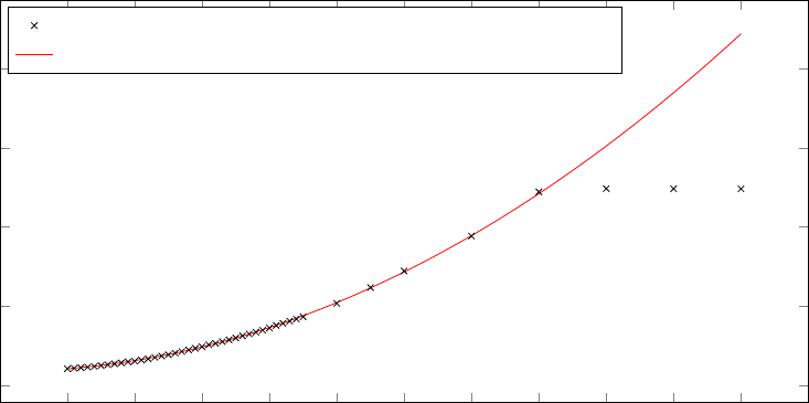
−100 0 100 200 300 400 500 600 700 800 900 1,000 1,100

100

150

200

Number of ASes

Memory consumed (GB)

Test results

Memory (kB) = 178.23 ∗ x

+ 33, 058.91 ∗ x + 10, 566, 441

Figure 14: Number of ASes vs. memory consumption

with a function is also shown on the graph. Since the host memory is 128 GB, it reaches the physical

limit after the test of 700 autonomous systems. The host system starts to swap the pages out to swap

spaces. Since the goal of the tests is to see per-unit performance without overloading the host, results

after 600 autonomous systems are not used in the graph ﬁtting.

The function used to ﬁt the graph is y = 178.23 ∗ x

+ 33, 058.91 ∗ x + 10, 566, 441, where y is the

memory consumption in kB. This function makes sense because:

• The host system itself consumes a ﬁxed amount of memory even when it is not doing anything.

This is the constant part of the function (i.e., the 10, 566, 441 kB here. This is the same memory

consumption when the host system is not running any emulation).

• When containers are not running anything, it is also reasonable to assume that they will consume

some memory. In this case, every router and route server is also running the BIRD routing daemon.

The host system also needs some amount of memory to just have the namespaces for containers.

Having bridges on the host system also consumes a bit of memory. This is the liner component in

the function (33, 058.91 ∗ x). This indicates a 33, 058.91 kB memory consumption for each router.

• For the 178.23∗x

part, it is safe to assume that this is the memory consumed by the routing table.

Since every router’s routing daemon and kernel routing table needs to install the routes advertised

by every other router, the x

makes sense. In this case, the 178.23 kB is the memory needed for a

single network.

Figure 15 shows the relationship between the number of autonomous systems and CPU time in

seconds. The horizontal axis is the number of autonomous systems, and the vertical axis is the CPU

time in seconds that the CPU spent in a non-idle state. A liner function, y = 0.063 ∗ x + 3, is used to ﬁt

−100 0 100 200 300 400 500 600 700 800 900 1,000 1,100

500

1,000

1,500

2,000

Number of ASes

CPU time (s)

Test results

y = 0.063 ∗ x + 3

CPU usage (%)

Figure 15: Number of ASes vs. CPU time

the test results. One may notice that the CPU time goes up signiﬁcantly after 700 autonomous systems.

Recall that the host reaches the physical memory limit after 700 autonomous systems. Many CPU times

are spent swapping pages in and out of the physical memory, and therefore the explosion of CPU time

after 700. Another ﬁgure, Figure 16 is provided to show the trend before hitting the physical limit. It

should also be noted that the CPU is still not in full load even when running out of physical memory

and having to resort to swapping (peak at 32.3956%), so one may, in theory, run large emulation given

that they have a fast enough swap space and CPU.

Figure 16 shows a near-linear relation in CPU time against the number of autonomous systems.

This result makes sense since once the route propagation completes, there will rarely be new CPU-heavy

tasks in the emulation since there are no host nodes, only router nodes. The CPU time can be seen

ﬂuctuating a bit throughout the tests. One possible exploration for this behavior is that, since the CPU

time is rather low to start with, any instability in the host system or the containers can be reﬂected on

the result as a rather large change in the CPU time. One example of this source of instability is how the

kernel scheduler decides to run the containers. The main CPU consumer, in this case, is observed to be

the routing daemon. Since OSPF is enabled on every router, even when they do not have any neighbors,

they still send out periodic OSPF hellos over the internal networks, leading to some CPU consumption.

BGP is also sending periodic keep-alive messages. The CPU usage also never exceeds 1%, so it is less of

a concern in this case when compared with the memory usage.

9.3.2 Large number of hosts

This section focuses on the memory consumption of the host nodes running some lightweight services.

The number of autonomous systems, routers, and autonomous systems in each Internet exchange is ﬁxed

−50 0 50 100 150 200 250 300 350 400 450 500 550 600 650

Number of ASes

CPU time (s)

Test results

y = 0.063 ∗ x + 3

0.2

0.4

0.6

0.8

CPU usage (%)

Figure 16: Number of ASes vs. CPU time (when memory is suﬃcient)

to ten, one, and ﬁve, respectively. Every host node in the emulator will run a nginx web server and run

ping against one random router in the emulator. The scripts in listing 75 and 76 is used to generate the

emulation.

The test will start from 0 host nodes as a baseline and continue until 80 hosts. It should be noted

that, unlike the last test, 0 host nodes here does not mean the host system is not running an emulation. It

means the emulation is running ten autonomous systems, each with one router and one internal network

but no hosts. It should also be noted that the same number of hosts are created in every internal network

in every autonomous system. For example, if eighty hosts are created for each autonomous system, the

total for ten autonomous systems will be 800 hosts.

Unlike the last test, where the max number of routers is 1,000, this test only goes to 800 to ensure

that the emulation will not require more than the physical memory the host has to run.

From Figure 17, one can see that the memory consumption for host nodes is nearly perfectly linear.

This result also makes sense, as adding new host nodes is merely creating a new container in the emulation

that runs some software. In this case, the software running on the host node operates individually (ping

and nginx), meaning adding a new instance of the software does not make any diﬀerence to the existing

instance of the software. In the last test, each new autonomous system generates a new route that needs

to be installed to every router, and therefore the quadratic component of ﬁt function.

The ﬁt function is y = 615 ∗ x + 47, 389.91. Here, 47, 389.91 is the memory in MB when no host is

running in any autonomous system. The 615 MB is the memory in kB required to run ten host nodes

with ping and nginx. That means 61.5 MB each hosts.

Figure 18 plots the relationship between numbers of host nodes and CPU time. The result again

shows a linear pattern with some ﬂuctuation. The ﬂuctuations are likely introduced by the same factors

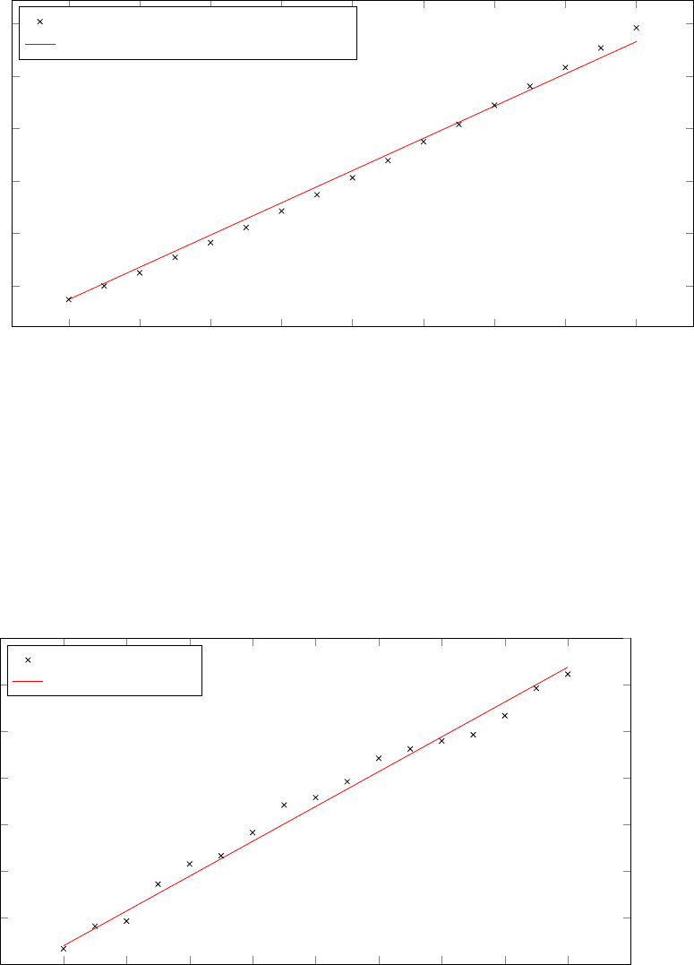
0 10 20 30 40 50 60 70 80

100

Number of hosts per AS (the total number of ASes is 10)

Memory consumed (GB)

Test results

Memory (MB) = 615 ∗ x + 47, 389.91

Figure 17: Number of hosts per AS vs. memory consumed

−10 0 10 20 30 40 50 60 70 80 90

Number of hosts per AS (the total number of ASes is 10)

CPU time (s)

Test results

y = 0.75 ∗ x + 3.92

0.2

0.4

0.6

0.8

1.2

1.4

CPU usage (%)

Figure 18: Number of hosts per AS vs. CPU time

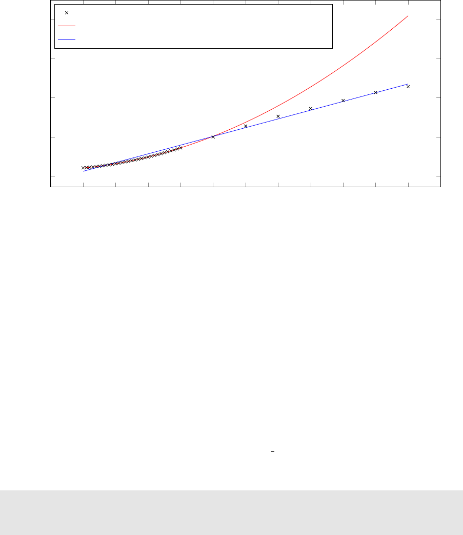
−10 0 10 20 30 40 50 60 70 80 90 100 110

100

150

200

Number of routers per AS (the total number of ASes is 10)

Memory consumed (GB)

Test results

(kB) = 15, 469.49 ∗ x

+ 388, 428.37 ∗ x + 10, 573, 163

(kB) = 1, 110, 000 ∗ x + 6, 342, 004

Figure 19: Number of routers per AS vs. memory consumed

as the last test. In the ﬁt function, 3.92 second is the CPU time spent when there is no host running.

On average, ten host nodes running ping and nginx consume 0.75 seconds of CPU time. In other words,

0.075 seconds for each host node. It is higher than the 0.063 of routers; one possible explanation of this

is that, with the hosts pinging routers, the ICMP packet may travel more than one hop, whereas the

OSPF hellos and BGP keepalives are only sent to the directly connected networks. Again, the CPU

usage is under 1.5% percent the whole time, so it is not the primary concern.

The ARP cache issue During the test case for 80 host nodes, the Linux kernel started to report

ARP table overﬂow. Sample error messages are shown in listing 74 This is due to the low default ARP

table size settings. This setting can be changed using the gc thresh parameters [28].

Listing 74: Linux ARP table overﬂow

[282667.265515] neighbour: arp_cache: neighbor table overflow!

[282667.265587] neighbour: arp_cache: neighbor table overflow!

[282667.265659] neighbour: arp_cache: neighbor table overflow!

[282671.169367] net_ratelimit: 20 callbacks suppressed

9.3.3 Large number of networks, but small amount of autonomous systems

This test looks at the unit performance when the number of autonomous systems is small, but each

autonomous system has a lot of internal routers and a lot of internal networks. In this test, there are

ten autonomous systems and ﬁve autonomous systems in each Internet exchange. There will be 1 to 90

routers in each autonomous system. Recall that the number of the network in each autonomous system

is 2 ∗ n

router

− 1. So at peak, there will be 1,790 networks (not counting the Internet exchange).

Figure 19 shows the memory consumption plotted against the number of routers within each au-

100

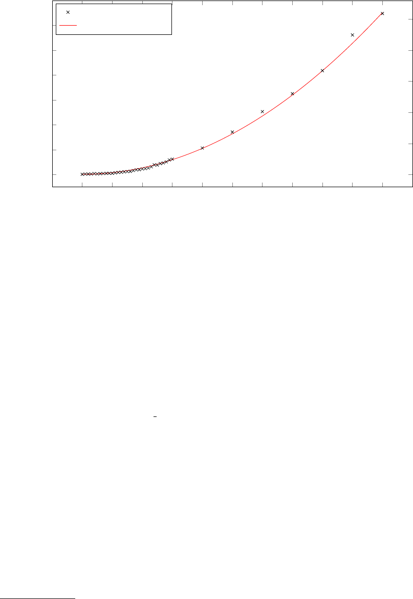
−10 0 10 20 30 40 50 60 70 80 90 100 110

200

400

600

800

1,000

1,200

1,400

Number of routers per AS (the total number of ASes is 10)

CPU time (s)

Test results

y = 0.13 ∗ x

+ 3.38

CPU usage (%)

Figure 20: Number of routers per AS vs. CPU time

tonomous system. Two ﬁts were attempted on the test results, one using the results for 0 to 30 routers

and the router using results for 30 to 100 routers. One may observe that the memory consumption starts

showing a quadratic-like trend when the number of routers is small (for example, the 0 to 10 routers

range) and looks like a linear trend as the number of routers increases. One reason for this is that, as

the number of routes from the same autonomous system increases, the number of memory consumed

per route will decrease. BIRD uses an eﬃcient way to store routes, where routes with the same route

attribute will be “combined.” [9] Routes from the same autonomous system, in this case, will share the

same set of attributes (ORIGIN, AS PATH, and NETHOP). BIRD can therefore store only the preﬁx and

only keep one copy of the route attributes. Ideally, there will only be ten unique copies from diﬀerent

autonomous systems; all routes from the same autonomous systems should share the same attributes.

While the preﬁx itself still needs to be stored on every router, given its small size (32 bits for the preﬁx

and 8 bits for the preﬁx length), the consumption of the route itself may be overshadowed by other major

memory consumers like the OSPF and IBGP sessions themselves.

Figure 20 shows the relationship between numbers of routers and CPU time. It follows a quadratic

trend, which makes sense. Since the IBGP layer conﬁgures full-mesh IBGP between all reachable

internal routers, the number of IBGP sessions pairs in terms of the number of routers is n

paris

(

router

∗(n

router

−1)

), therefore the quadratic trend. Figure 21 shows the relationship between the number

of IBGP sessions and CPU time, and one can clearly see the linear relationship now. One may realize

that OSPF may also contribute to the CPU time here; however, since there are only two OSPF-enabled

interfaces on most routers, and with the number of IBGP sessions going up to 99,000, the CPU time

consumed by OSPF is not as signiﬁcant.

Note that this test is done using the full-mesh IBGP setup. If one chooses to use the MPLS option,

101

−0.1 0 0.1 0.2 0.3 0.4 0.5 0.6 0.7 0.8 0.9 1 1.1

·10

200

400

600

800

1,000

1,200

1,400

Number of IBGP sessions

CPU time (s)

Test results

y = 0.0134 ∗ x + 3.38

CPU usage (%)

Figure 21: Number of IBGP sessions vs. CPU time

all non-core routers will no longer carry the full table. In fact, they will not run IBGP at all. This should

reduce the memory and CPU consumption signiﬁcantly. One other option to reduce CPU consumption

is to use the route-reﬂector-based IBGP, which will reduce the number of IBGP sessions to only n

session, where n is the number of internal routers. There may not be signiﬁcant changes to the memory

consumption, but it should have a great impact on CPU consumption.

Figure 21 also provide valuable information regarding the CPU consumption of BGP sessions them-

selves. IBGP and EBGP are, in nature, the same, and therefore the test provides an option for one to

evaluate how many sessions one can expect to run, given the CPU hardware.

9.3.4 Packet forwarding

This section focuses on the packet forwarding performance of the emulator. In addition to CPU and

memory, tests in this section also run iperf3 and ping between nodes to test throughput and latency

between nodes. iperf3 is a network benchmarking tool that can be used to measure the throughput of

the network. The scripts in listing 80 and 81 are used generating emulation for the tests.

Single path, single connection, various numbers of hops In this set of tests, only one autonomous

system is created. In each autonomous system, there are 10 to 200 internal networks. Another emulation

generator script generates the tests. One router will sit between two internal networks. Two hosts sit at

the edge of the long chain of routers and networks. The hosts are conﬁgured to use 255 as their default

TTL to allow their packet to traverse the long path. The host uses the default TCP congestion control

algorithm (cubic). ipref3 is used to test the TCP TX and RX speed using a single connection. ping

is used to test the RTT (Round-trip time) between the two hosts. ping is conﬁgured to send one ICMP

102

0 20 40 60 80 100 120 140 160 180 200

1,000

2,000

3,000

4,000

Number of hops

Throughput (Mbps)

y =

41,137

− 350

Figure 22: Number of hops vs. TX/RX speed

echo every millisecond. The ping program will send a total of 1,000 ping packets.

Figure 22 shows the relationship between transmit (TX) and receive (RX) speed over a single TCP

connection and the numbers of hops in between the sender and receiver. The relationship appears

hyperbolic. Considering that some ﬁxed overhead and slowdown will occur on every hop the packet

traverse, this outcome makes sense.

Figure 23 shows the relationship between RTT and the number of hops in between. The relationship

appears to be quadratic. On paper, this relationship should be linear. The reason for it being quadratic is

likely again IBGP and OSPF. IBGP keepalives use CPU resources, and there will be again n ∗(n−1) IBGP

sessions, where n is the number of the routers. Since the number of networks within the autonomous

system increased, OSPF may also contribute a higher amount of CPU usage in this case. With most

CPU time spent in OSPF and IBGP, as the number of hops increase, the more time the ICMP packet

needs to wait before it gets transmitted.

Multiple parallel streams The next set of tests benchmarks the packet forwarding performance when

multiple pairs of clients and servers send traﬃc to each other. In tests, 1 to 20 autonomous systems are

created. In each autonomous system, there are ten routers between the client and the server. The client

and server will perform the same set of tests as the last case (i.e., throughput and ping), but with 1 to

20 pairs of client and server simultaneously.

Figure 24 shows the relationship between number of parallel streams and throughput. The relation-

ship appears logarithmic. With each additional new pair of client and server, the throughput increase

to some extent, but the increase in throughput drops as the number of streams go up. One may also

notice that the speed stopped increasing at around 11 streams at around 13 Gbps. At the same time,

when it reaches 13 Gbps, the CPU usage on all cores reaches around 100%. This indicates a hardware

103

0 20 40 60 80 100 120 140 160 180 200

Number of hops

Average RTT (ms)

RTT

y = 0.00065 ∗ x

+ 0.02720 ∗ x

Figure 23: Number of hops vs. RTT

0 2 4 6 8 10 12 14 16 18 20

Number of streams (the number of hops is 10)

Total throughput (Gbps)

y (Mbps) = 3, 900 ∗ ln(x) + 3, 900

Figure 24: Number of streams vs. TX/RX speed

104

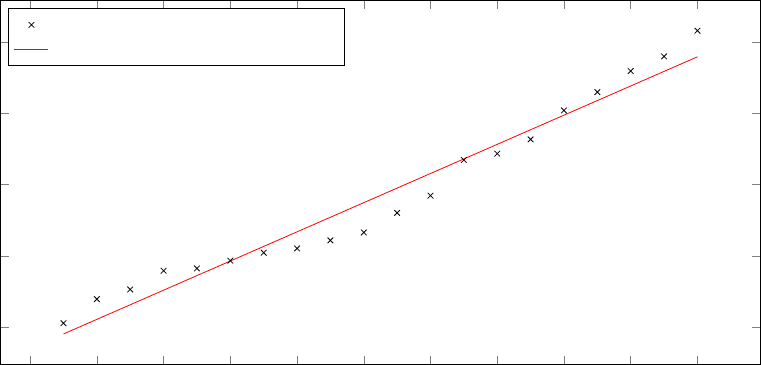
0 2 4 6 8 10 12 14 16 18 20

0.4

0.6

0.8

1.2

Number of streams (the number of hops is 10)

Average RTT (ms)

RTT

y = 0.04088755 ∗ x + 0.33995113

Figure 25: Number of streams vs. RTT

performance limit.

Figure 25 shows the RTT and its relationship with the number of parallel streams. Even when it

reaches 20 streams (or 200 routers), the RTT is still below 1.5ms. The relationship itself appears linear.

Unlike the last test, the total number of IBGP sessions is much smaller since each autonomous system

only has ten routers. At peak, there are only 10 ∗ (10 − 1) ∗ 20 = 1800 IBGP sessions, as opposed to

200 ∗ (200 − 1) = 39800 IBGP sessions in the last test. This shows that without IBGP contributing to

the large CPU usage, the RTT itself only increases linearly as the number of nodes in the emulation

increases.

9.3.5 Smaller scale tests

In order to conﬁrm the trends above and see how a more typical personal computer performs when

using the emulator, a select sets of the tests above are repeated on a virtual machine with the following

hardware:

• 2 * Intel

Xeon

Silver 4210 CPU @ 2.00GHz virtual CPUs

• 4 GB of DDR4 memory

The above hardware is a more realistic representation of what an average SEEDEMU personal user

may use. The same tests are performed on the virtual machine. This section will cover the results of the

tests. The swapness value is again set to 1.

Memory vs. number of autonomous systems This is the same test, but it only goes up to 100

autonomous systems instead of 1,000 in this round.

105

−10 0 10 20 30 40 50 60 70 80 90 100 110

1,000

2,000

3,000

4,000

5,000

Number of ASes

Memory consumed (MB)

Test results

Memory (kB) = 178.23 ∗ x

+ 33, 058.92 ∗ x + 278, 342

Figure 26: Number of ASes vs. memory consumption

Figure 26 shows the consumption in small scale test. The same quadratic function from the last test

was reused, except that the constant part has been changed to match the idle host memory consumption.

It can be seen in the ﬁgure that the function predicted the memory consumption pretty accurately.

However, the virtual machine reaches the physical memory limit at around 80 autonomous systems and

starts to swap.

Figure 27 shows the CPU usage. The relationship is linear, but the CPU time does not increase as

rapidly as the last test. The reason may be that the Xeon

Silver 4210 CPU is superior to the E5-2660.

The CPU usage still spikes up after it swaps pages out, but the eﬀect is much less intensive. Possible

reasons are that fewer pages need to be swapped out (the overall memory usage is low) and that the

storage medium is M.2 SSD instead of HDD in the last test. Again, the CPU load is too low to be the

limiting factor. The primary limiting factor is memory consumption.

Forwarding - number of hops Figure 28 shows the test result of the same throughput speed tests,

but only goes up to 100 hops. The pattern is again hyperbolic. The initial speed goes up to 6,850 Mbps,

likely due to the higher CPU power available for the emulator. The throughput at 100 hops is 8.18 Mbps.

Figure 29 shows the relationship between RTT and number of hops. The relationship is again

quadratic but is lower overall, likely also due to the faster CPU.

Forwarding - parallel streams Figure 30 shows the same parallel forwarding throughput test. The

pattern here is very diﬀerent from when testing with many CPU cores. Here, the performance may be

limited by the test program, iperf3, rather than the actual packet forwarding. One can observe that the

test yields the highest throughput when using two threads, which may be because there are two virtual

CPU cores allocated to the virtual machine. Having too many parallel streams, instead of increasing

106

−10 0 10 20 30 40 50 60 70 80 90 100 110

0.5

1.5

2.5

Number of ASes

CPU time (s)

Test results

y = 0.018 ∗ x + 0.595960

0.2

0.4

0.6

0.8

1.2

1.4

CPU usage (%)

Figure 27: Number of ASes vs. CPU time

10 20 30 40 50 60 70 80 90 100

2,000

4,000

6,000

Number of hops

Throughput (Mbps)

y =

75,500

− 850

Figure 28: Number of hops vs. TX/RX speed

107

10 20 30 40 50 60 70 80 90 100

Number of hops

Average RTT (ms)

RTT

y = 0.00046108 ∗ x

Figure 29: Number of hops vs. RTT

the throughput, actually lowers the throughput. A possible explanation of such behavior may be in the

scheduling. Having too many sets of iperf3 makes the operating system constantly context switching

from one test program to the other, lowing eﬃciency.

Figure 31 shows the relationship between RTT and the number of parallel pings. The test result

falls within 0.22 ms and 0.32 ms, which is within the margin of error. There are just not enough nodes

to have an impact on the RTT with this stronger CPU.

9.4 Conclusion

The evaluation section ﬁnds that the design of SEEDEMU matches all design goals. The test section

conducted various tests and found out the following per-unit performance functions:

• Memory vs. autonomous system with one network (i.e., network with unmergeable attributes):

memory = 178.23 × x

+ 33, 058.91 × x + C.

• CPU time vs. autonomous system with one network: time = k × x + C.

• Memory vs. host running some simple service: memory = 615, 000 × n

host

+ C.

• CPU time vs. host running some simple service: time = k × n

host

+ C.

• Memory vs. autonomous system with a lot of routers, given large enough number of routers (i.e.,

a lot of networks with mergeable attributes): memory = 111, 000 × n

router

+ C.

• CPU vs. autonomous system with a lot of networks: time = k × x

+ C.

• CPU vs. Number of BGP sessions: time = k × n

session

+ C.

108

1 2 3 4 5 6 7 8 9 10

0.2

0.4

0.6

0.8

1.2

1.4

·10

Number of streams (the number of hops is 10)

Total throughput (Mbps)

Figure 30: Number of streams vs. TX/RX speed

1 2 3 4 5 6 7 8 9 10

0.22

0.24

0.26

0.28

0.3

0.32

Number of streams

Average RTT (ms)

Figure 31: Number of streams vs. RTT

109

• RTT vs. number of hops: rtt = k

× n

hops

+ k

× n

hops

+ C.

. . . where k and C are some constant. k and C may vary from system to system. k is added under

the assumption that, given the architectures do not vary too much, other CPUs may be able to run all

codes faster or slower, so the speedup and slowdown should be constant. C is the idle CPU / memory

consumption for the system. Another set of tests may be required if the CPU architecture changes

too much and the speedups and slowdowns of certain tasks are greater than the others. The memory

consumption should be constant unless there are drastic changes in hardware architecture or optimization

of BIRD, Linux kernel, or docker.

In most tests, the bottleneck is at memory since the emulation node uses only a tiny amount of

CPU compared with the amount of memory they used. Unless one is performing heavy tasks inside the

emulator, like running Ethereum miner, they are most likely to hit the physical memory limit before

they hit the CPU limit. The tests provided a function to approximate the number of networks they can

run based on available physical memory.

10 Summary and future work

The SEEDEMU framework is a programming framework that allows one to build network emulations

easily. While there are plenty of emulation platforms, there are no convenient ways to build emulations

for those said platforms. Some existing platforms also have limited scalability, and it is demonstrated that

the main target platform of the SEEDEMU framework, docker, is scalable enough to handle extensive

emulations given enough hardware resources.

This thesis explored the current network emulations and simulation solutions, identiﬁed the missing

piece in them to make them suitable for for-education use (namely, ease of use when building large

emulation, reusability, and scalability), and tackled every critical missing piece to produce a very easy-

to-use framework that exceeds the original design goals. The thesis went through the entire design

process of the SEEDEMU framework, detailed and justiﬁed the design choices, and explored diﬀerent

approaches to non-trivial tasks.

10.1 Future work

While I believe the SEEDEMU framework is already in excellent shape, here are a few improvements

that can make it even more powerful and useful.

Topology generator Sometimes, one may want to experiment with some high-level application on the

emulator, like DNS infrastructure, blockchain, and more. Now, in order to use those high-level services,

one would need to ﬁrst build or obtain a pre-built base layer image.

110

The BGP information is generally publicly available via countless public looking glasses on the

Internet, and some public services, like R´eseaux IP Europ´eens Network Coordination Centre Routing

Information Service

, even program programmatic API access to BGP information. Other publicly

available information like PeeringDB

also provides information of private and public peering facilities,

Internet exchange members, etc. It is possible to build an emulation generator that generates base layer

topology based on publicly available information. The emulation may not necessarily be the exact replica

of the real world, but it should provide real enough experience for one who wants to test higher-level

services.

Web-UI extensions The web UI currently oﬀers “quick actions” to enable and disable BGP peers or

disconnect a node from the network entirely. The logic of those quick actions is currently implemented

by the docker compiler and the client program. Meaning to add new quick actions, one will have to

update the client program and the compiler. As most users will probably use the map feature of the

seedemu-client to interact with the emulation, it can be a good idea to provide some API to allow layers

and services to provide their own quick actions on the map.

Some possible use cases include:

• One may be interested in using the emulator for smart contact, but they may not know how to

operator BGP/OSPF (i.e., work with the BIRD CLI or vtysh). They, however, may be interested

to see how disconnecting major ISPs from networks aﬀect the blockchain. Quick actions will allow

them to do that without knowing how to operate the CLI.

• Some services, like botnet and Ethereum, take user interaction after the emulation is started.

Providing quick actions allows them to interact without having prior knowledge on how to operate

the software (the botnet control server and geth in this case). This can be the extent to other

services, like DNS, to dynamically create new zones, conﬁgure Negative Trust Anchors [29], and

more.

Improved distributed emulation While the SEEDEMU framework provides the compiler to output

emulation that can be run distributed on a docker swarm cluster; the current option is somewhat limited.

For starters, the web UI program will only be able to see networks and nodes running on the current

cluster node, not the entire cluster. It is also currently only possible to break emulation at the autonomous

system level. One may want to break the emulation down into a ﬁner faction, or based on other criteria,

like geographic region, and more.

https://www.ripe.net/analyse/Internet-measurements/routing-information-service-ris

https://www.peeringdb.com

111

More services and components Developing new services and components for the framework is a

continuous eﬀort. More services and components can be added to the emulator to allow one to cover

more areas of interest.

Other compilers While the emulator itself focuses mainly on docker. It could also be helpful to add

other compilers. Like Kubernetes, LXC, or even other network emulation software. As time goes on,

there may also be superior emulation platforms available. Developing from the new platforms to archive

greater performance is also a continuous eﬀort.

Unit tests The SEEDEMU framework is an open-source project. In order to attract outside contrib-

utors, it is important that there are some ways for the contributors to check their contributions. While

it is possible to review every change manually, it will quickly become very tedious if the number of

contributors increases. Some unit tests to automate common checks should be developed for the project.

11 Appendix

11.1 Perform the evaluation locally

This section details how one can use the benchmark script to perform the same tests in the performance

evaluations section and how to process the raw data from /proc/meminfo and /proc/stat, etc.

There are two emulator generator scripts used; one for generating an emulation with large numbers

of networks and nodes, and one for generating one or multiple long chains of networks. There are also

two driver scripts that invoke the two emulation generator scripts and collect stats like CPU, memory,

ping output, and iperf3 output. Finally, two scripts are used to process the raw data collected by the

emulation generator and output the data in CSV format. The next two subsections will go over the

implementation and usage of the scripts.

11.1.1 CPU and memory usage

The section describes the scripts used to generate emulation and collecting metrics with large numbers

of nodes and networks.

Emulation generation script Listing 75 shows the code for the “large numbers of routers, hosts

and/or autonomous systems” emulator generator. This generator takes the following parameters:

• --ases: Number of autonomous systems to generate.

• --ixs: Number of autonomous systems in each internet exchange. The number of internet ex-

changes equals the number of autonomous systems divided by the number of autonomous systems

112

in each internet exchange.

• --routers: Number of routers to create in each autonomous system. One internal network is

created with each router. If the number of routers is greater than two, an additional network

will be created between the routers. A router connects to at least one network (only the internal

network) and at most three networks (one internal and two networks connecting to two other

routers.)

• --hosts: Number of host nodes to put in each internal network.

• --web: Run a web server on every host node created.

• --ping: Let every host node ping a random router in the emulator.

• --outdir: The directory to store the generated emulation.

For example, to generate an emulation with 100 autonomous systems, each with ten routers, each

with ten hosts in their internal network, one can run the following command:

./generator-1.py --ases 100 --ixs 10 --routers 10 --hosts 10 --outdir ./out

The emulation will be saved in the ./out directory. One can cd into the output folder and run

docker-compose up to start it.

Listing 75: Emulation generator: Large numbers of routers, hosts and/or autonomous systems

#!/usr/bin/env python3

from seedemu import *

from typing import List, Dict, Set

from ipaddress import IPv4Network

from math import ceil

from random import choice

import argparse

def createEmulation(asCount: int, asEachIx: int, routerEachAs: int, hostEachNet: int,

hostService: Service, hostCommands: List[str], hostFiles: List[File], yes: bool) ->

Emulator:

asNetworkPool = IPv4Network('16.0.0.0/4').subnets(new_prefix = 16)

linkNetworkPool = IPv4Network('32.0.0.0/4').subnets(new_prefix = 24)

ixNetworkPool = IPv4Network('100.0.0.0/13').subnets(new_prefix = 24)

ixCount = ceil(asCount / asEachIx)

rtrCount = asCount * routerEachAs

hostCount = asCount * routerEachAs * hostEachNet + ixCount

netCount = asCount * (routerEachAs + routerEachAs - 1) + ixCount

print('Total nodes: {} ({} routers, {} hosts)'.format(rtrCount + hostCount, rtrCount,

hostCount))

print('Total nets: {}'.format(netCount))

if not yes:

input('Press [Enter] to continue, or ^C to exit ')

113

aac = AddressAssignmentConstraint(hostStart = 2, hostEnd = 255, hostStep = 1, routerStart

= 1, routerEnd = 2, routerStep = 0)

assert asCount <= 4096, 'too many ASes.'

assert ixCount <= 2048, 'too many IXs.'

assert hostEachNet <= 253, 'too many hosts.'

assert routerEachAs <= 256, 'too many routers.'

emu = Emulator()

emu.addLayer(Routing())

emu.addLayer(Ibgp())

emu.addLayer(Ospf())

if hostService != None:

emu.addLayer(hostService)

base = Base()

ebgp = Ebgp()

ases: Dict[int, AutonomousSystem] = {}

asRouters: Dict[int, List[Router]] = {}

hosts: List[Node] = []

routerAddresses: List[str] = []

# create ASes

for i in range(0, asCount):

asn = 5000 + i

asObject = base.createAutonomousSystem(asn)

ases[asn] = asObject

asRouters[asn] = []

localNetPool = next(asNetworkPool).subnets(new_prefix = 24)

# create host networks

for j in range(0, routerEachAs):

prefix = next(localNetPool)

netname = 'net{}'.format(j)

asObject.createNetwork(netname, str(prefix), aac = aac)

router = asObject.createRouter('router{}'.format(j))

router.joinNetwork(netname)

routerAddresses.append(str(next(prefix.hosts())))

asRouters[asn].append(router)

# create hosts

for k in range(0, hostEachNet):

hostname = 'host{}_{}'.format(j, k)

host = asObject.createHost(hostname)

host.joinNetwork(netname)

if hostService != None:

vnode = 'as{}_{}'.format(asn, hostname)

hostService.install(vnode)

emu.addBinding(Binding(vnode, action = Action.FIRST, filter = Filter(asn =

asn, nodeName = hostname)))

hosts.append(host)

for file in hostFiles:

path, body = file.get()

host.setFile(path, body)

114

routers = asRouters[asn]

# link routers

for i in range (1, len(routers)):

linkname = 'link_{}_{}'.format(i - 1, i)

asObject.createNetwork(linkname, str(next(linkNetworkPool)))

routers[i - 1].joinNetwork(linkname)

routers[i].joinNetwork(linkname)

lastRouter = None

asnPtr = 5000

ixMembers: Dict[int, Set[int]] = {}

# create and join exchanges

for ix in range(1, ixCount + 1):

ixPrefix = next(ixNetworkPool)

ixHosts = ixPrefix.hosts()

ixNetName = base.createInternetExchange(ix, str(ixPrefix), rsAddress =

str(next(ixHosts))).getPeeringLan().getName()

ixMembers[ix] = set()

if lastRouter != None:

ixMembers[ix].add(lastRouter.getAsn())

lastRouter.joinNetwork(ixNetName, str(next(ixHosts)))

for i in range(1 if lastRouter != None else 0, asEachIx):

router = asRouters[asnPtr][0]

ixMembers[ix].add(router.getAsn())

router.joinNetwork(ixNetName, str(next(ixHosts)))

asnPtr += 1

lastRouter = router

# peerings

for ix, members in ixMembers.items():

for a in members:

for b in members:

peers = ebgp.getPrivatePeerings().keys()

if a!= b and (ix, a, b) not in peers and (ix, b, a) not in peers:

ebgp.addPrivatePeering(ix, a, b, PeerRelationship.Unfiltered)

# host commands

for host in hosts:

for cmd in hostCommands:

host.appendStartCommand(cmd.format(

randomRouterIp = choice(routerAddresses)

), True)

emu.addLayer(base)

emu.addLayer(ebgp)

return emu

def main():

parser = argparse.ArgumentParser(description='Make an emulation with lots of networks.')

parser.add_argument('--ases', help = 'Number of ASes to generate.', required = True)

parser.add_argument('--ixs', help = 'Number of ASes in each IX.', required = True)

parser.add_argument('--routers', help = 'Number of routers in each AS.', required = True)

parser.add_argument('--hosts', help = 'Number of hosts in each AS.', required = True)

parser.add_argument('--web', help = 'Install web server on all hosts.', action =

'store_true')

115

parser.add_argument('--ping', help = 'Have all hosts randomly ping some router.', action =

'store_true')

parser.add_argument('--outdir', help = 'Output directory.', required = True)

parser.add_argument('--yes', help = 'Do not prompt for confirmation.', action =

'store_true')

args = parser.parse_args()

emu = createEmulation(int(args.ases), int(args.ixs), int(args.routers), int(args.hosts),

WebService() if args.web else None, ['{{ while true; do ping {randomRouterIp}; done }}']

if args.ping else [], [], args.yes)

emu.render()

emu.compile(Docker(selfManagedNetwork = True), args.outdir)

if __name__ == '__main__':

main()

Automating the tests and collecting metrics Listing 76 provides an automated way to test and

collect metrics using the emulator generator script above. It reads options from the environment. The

accepted environment variables are:

• TARGET: Test target. Can be ases, routers and hosts. Diﬀerent number of TARGETs will be

created using the generator script.

• START: Number of targets to start the test from.

• END: Number targets to end the test at.

• STEP: Number of increments in the number of targets in each step.

The number of autonomous systems in each exchange is ﬁxed to ﬁve in all tests.

Listing 76: Driver script: Large numbers of routers, hosts and/or autonomous systems

#!/bin/bash

SAMPLE_COUNT='100'

set -e

cd "`dirname "$0"`"

results="`pwd`/results"

[ ! -d "$results" ] && mkdir "$results"

function collect {

for j in `seq 1 $SAMPLE_COUNT`; do {

now="`date +%s`"

echo "[$now] snapshotting cpu/mem info..."

cat /proc/stat > "$this_results/stat-$now.txt"

cat /proc/meminfo > "$this_results/meminfo-$now.txt"

sleep 1

}; done

}

116

for ((i=${START}; i<=${END}; i+=${STEP})); do {

rm -rf out

echo "generating emulation..."

[ "$TARGET" = "ases" ] && \

./generator-1.py --ases $i --ixs 5 --routers 1 --hosts 0 --outdir out --yes

[ "$TARGET" = "routers" ] && \

./generator-1.py --ases 10 --ixs 5 --routers $i --hosts 0 --outdir out --yes

[ "$TARGET" = "hosts" ] && \

./generator-1.py --ases 10 --ixs 5 --routers 1 --hosts $i --outdir out --yes

this_results="$results/bench-$i-$TARGET"

[ ! -d "$this_results" ] && mkdir "$this_results"

pushd out

echo "buliding emulation..."

docker-compose build

# bugged? stuck forever at "compose.parallel.feed_queue: Pending: set()"...

# docker-compose up -d

# start only 10 at a time to prevent hangs

echo "start emulation..."

ls | grep -Ev '.yml$|^dummies$' | xargs -n10 -exec docker-compose up -d

echo "waiting 300s for ospf/bgp, etc..."

sleep 300

collect

docker-compose down

popd

}; done

One trick being used here worth mentioning is the following line:

Listing 77: Trick: start only ten containers at a time

ls | grep -Ev '.yml$|^dummies$' | xargs -n10 -exec docker-compose up -d

The docker-compose utility appears to have some issues when a lot of containers are deﬁned and

when it tries to start a lot of containers at once. The line in listing 77 makes the docker-compose utility

only starts ten containers at a time and therefore prevent it from freezing. At the time of writing, this

issue is unsolved

For example, to perform tests from 10 to 100 autonomous systems and increment the number of

autonomous systems in each step by 10, one can do:

TARGET=ases START=10 END=100 STEP=10 ./driver-1.sh

The driver script will invoke the generator script, create and start the emulation, wait for 300

seconds

to make sure the routing converges, then start collecting metrics from the /proc/stat and

/proc/meminfo ﬁle once every second for 100 seconds. The results are stored in:

• ./results/bench-$i-$TARGET/stat-$now.txt

• ./results/bench-$i-$TARGET/memnifo-$now.txt

https://github.com/docker/compose/issues/7577

It is tested that even with more than 1,000 autonomous systems, the routing converges in under 250 seconds.

117

. . . where $i is the number of targets (a number between 10 and 100, in this case), $TARGET is the

test target (ases, in this case), and $now is the Unix epoch time when the metric is collected. Once

100 samples of metrics are collected, the driver script will stop the emulation and do the test again with

more targets. This is repeated until the END is reached.

Processing the raw metrics Once the data are collected, another script can be used to generate a

summary of the data. Listing 78 shows the code for the script.

Listing 78: Summary script: Large numbers of routers, hosts and/or autonomous systems

#!/bin/bash

rsltdir="results/bench-*-$1"

echo "$1,memused,cpu_sec"

for report in $rsltdir; do {

head="`sed -n 's/.*bench-$[0-9]*$-.*/\1/p' <<< "$report"`"

memfree_avg="`cat "$report/"meminfo-* | grep MemFree | awk -v N=2 '{ sum += $N } END { if

(NR > 0) printf "%.0f", sum / NR }'`"

memtotal="`cat "$report/"meminfo-* | grep MemTotal | head -n1 | awk '{print $2}'`"

cputime_avg="`cat "$report/"stat-* | grep 'cpu ' | awk '{ print $2 + $3 + $4 + $7 + $8 +

$9 + $10 + $11 }' | awk '{ if (NR > 1) print $1-old; old = $1 }' | awk -v N=1 '{ sum += $N

} END { if (NR > 0) printf "%f", sum / NR }'`"

let memused_avg=$memtotal-$memfree_avg

echo "$head,$memused_avg,$cputime_avg"

}; done | sort -nt, -k1

This script computes the average memory usage in the 100 collected samples. It also computes the

average CPU time spent doing work. It takes one parameter, the aﬃx of the name of the folders (i.e.,

ases, hosts, or routers). The output looks like this:

Listing 79: Summary script: example output

$ ./mkreport-cpu-men ases

ases,memused,cpu_sec

0,285022,0.593961

10,895102,0.821183

20,1147904,0.9637

...

11.1.2 Packet forwarding

The section describes the scripts used to generate emulation and collecting metrics with a large number

of hops and parallel streams.

Emulation generation script Another emulation generation script is created to allow easy generation

of emulation with one or more long chains of networks. The “long chain” here means the traﬃc needs

118

to travel many router hops to reach its ﬁnal destinations. The goal of this script is to test the RTT and

throughput in relation to the number of hops and streams. This script takes the following parameters:

• --ases The number of autonomous systems to generate. Each autonomous system can have 1

to 254 routers (numbers speciﬁed by --hops) and two hosts. The ﬁrst host will send 1,000 ping

packets to the second host. The ping program is set to wait only 10 ms between each ICMP echo

packet. The ﬁrst host will also run two iperf3 rounds with the second host. The ﬁrst round is to

test the TX speed, and the second round is to test the RX speed. Both rounds use TCP.

• --hops The number of hops, in each of the generated autonomous systems, to generate in between

the two test hosts. The two hosts are conﬁgured to use a default TTL value of 255.

Listing 80 shows the code for the “long chain” generator.

Listing 80: Emulation generator: Large numbers of hops and/or streams

#!/usr/bin/env python3

from seedemu import *

from typing import List

import argparse

TEST_SCRIPT = '''\

#!/bin/bash

# wait for b to go online (mostly waiting for routing convergence).

while ! ping -t255 -c10 {remote}; do sleep 1; done

ping -c1000 -i.01 {remote} > /ping.txt

while ! iperf3 -c {remote} -t 60 > /iperf-tx.txt; do sleep 1; done

while ! iperf3 -Rc {remote} -t 60 > /iperf-rx.txt; do sleep 1; done

touch /done

'''

def createEmulation(asCount: int, chainLength: int) -> Emulator:

assert chainLength < 254, 'chain too long.'

emu = Emulator()

emu.addLayer(Routing())

emu.addLayer(Ibgp())

emu.addLayer(Ospf())

base = Base()

emu.addLayer(base)

for asnOffset in range(0, asCount):

asn = 150 + asnOffset

asObject = base.createAutonomousSystem(asn)

nets: List[Network] = []

lastNetName: str = None

for netId in range(0, chainLength):

netName = 'net{}'.format(netId)

net = asObject.createNetwork(netName)

119

nets.append(net)

if lastNetName != None:

thisRouter = asObject.createRouter('router{}'.format(netId))

thisRouter.joinNetwork(netName)

thisRouter.joinNetwork(lastNetName)

lastNetName = netName

hostA = asObject.createHost('a')

hostB = asObject.createHost('b')

netA = nets[0]

netB = nets[-1]

addressA = netA.getPrefix()[100]

addressB = netB.getPrefix()[100]

hostA.joinNetwork(nets[0].getName(), addressA)

hostB.joinNetwork(nets[-1].getName(), addressB)

hostA.addSoftware('iperf3')

hostB.addSoftware('iperf3')

hostA.appendStartCommand('sysctl -w net.ipv4.ip_default_ttl=255')

hostB.appendStartCommand('sysctl -w net.ipv4.ip_default_ttl=255')

hostB.appendStartCommand('iperf3 -s -D')

hostA.setFile('/test', TEST_SCRIPT.format(remote = addressB))

hostA.appendStartCommand('chmod +x /test')

hostA.appendStartCommand('/test', True)

return emu

def main():

parser = argparse.ArgumentParser(description='Make an emulation with a ASes that has long

hops and run ping and iperf across hosts.')

parser.add_argument('--ases', help = 'Number of ASes to generate.', required = True)

parser.add_argument('--hops', help = 'Number of hops between two hosts.', required = True)

parser.add_argument('--outdir', help = 'Output directory.', required = True)

args = parser.parse_args()

emu = createEmulation(int(args.ases), int(args.hops))

emu.render()

emu.compile(Docker(selfManagedNetwork = True), args.outdir)

if __name__ == '__main__':

main()

For example, to generate two autonomous systems, each with 100 hops between the hosts, one may

use:

./generator-2.py --ases 2 --hops 100 --outdir ./out

The emulation can again be started using the docker-compose up command. The results of ping

(/ping.txt) and iperf3 (/iperf-tx.txt and /iperf-tx.txt) are available under the root folder of

120

the ﬁrst host node. Another ﬁle, /done, will be created when all the tests ﬁnishes. When the /done ﬁle

is available, it is safe to collect the ﬁles from containers.

Automating the tests and collecting metrics Similar to the last generator, a script for automating

the test and metric collection is created.

The driver script takes the following environment variables:

• TARGET The test target. Can be either ases or hops. For the ases test, the number of hops is

ﬁxed to ten. For the hops test, the number of ases is ﬁxed to one.

• START: Number of targets to start the test from.

• END: Number targets to end the test at.

• STEP: Number of increments in the number of targets in each step.

Listing 81 shows the code for the “long chain” driver.

Listing 81: Driver: Large numbers of hops and/or streams

#!/bin/bash

set -e

cd "`dirname "$0"`"

results="`pwd`/results"

for ((i=${START}; i<=${END}; i+=${STEP})); do {

rm -rf out

echo "generating emulation..."

[ "$TARGET" = "ases" ] && ./generator-2.py --ases $i --hops 10 --outdir out

[ "$TARGET" = "hops" ] && ./generator-2.py --ases 1 --hops $i --outdir out

this_results="$results/bench-$i-fwd-$TARGET"

[ ! -d "$this_results" ] && mkdir "$this_results"

pushd out

echo "buliding emulation..."

docker-compose build

# bugged? stuck forever at "compose.parallel.feed_queue: Pending: set()"...

# docker-compose up -d

# start only 10 at a time to prevent hangs

echo "start emulation..."

ls | grep -Ev '.yml$|^dummies$' | xargs -n10 -exec docker-compose up -d

echo "wait for tests..."

sleep 500

host_ids="`docker ps | egrep "hnode_.*_a" | cut -d\ -f1`"

for id in $host_ids; do {

while ! docker exec $id ls /done; do {

echo "waiting for $id to finish tests..."

sleep 10

}; done

121

echo "collecting results from $id..."

docker cp "$id:/ping.txt" "$this_results/$id-ping.txt"

docker cp "$id:/iperf-tx.txt" "$this_results/$id-iperf-tx.txt"

docker cp "$id:/iperf-rx.txt" "$this_results/$id-iperf-rx.txt"

}; done

docker-compose down

popd

}; done

This script also uses the trick in listing 77 to start only ten containers at a time.

For example, to benchmark forwarding for 10 to 100 routers hops, one may do:

START=10 END=100 STEP=10 TARGET=hops ./driver-2.sh

The driver script will, again, invoke the generator script, create and start the emulation and wait

for 500 seconds

. It then starts collecting the output ﬁles from the containers and copy them to the

results directory:

• ./results/bench-$i-$TARGET/$id-iperf-tx.txt

• ./results/bench-$i-$TARGET/$id-iperf-rx.txt

• ./results/bench-$i-$TARGET/$id-ping.txt

. . . where $i is the number of targets (a number between 10 and 100, in this case), $TARGET is the

test target (hops, in this case), and $id is the ID of the container. Once the output of ping and iperf3

are collected, the driver script will stop the emulation, and do the test again with more targets. This is

repeated until the END is reached.

Processing the raw metrics Again, a script to generate the CSV report from the results is also

included. Listing 82 shows the source for the script.

Listing 82: Summary script: Large numbers of hops and/or streams

#!/bin/bash

rsltdir="results/bench-*-$1"

echo "$1,rx_mbps,tx_mbps,retr,ping"

for report in $rsltdir; do {

head="`sed -n 's/.*bench-$[0-9]*$-.*/\1/p' <<< "$report"`"

rx="`cat "$report/"*-iperf-rx.txt | grep receiver | awk '{print $7 * ($8 == "Gbits/sec" ?

"1000" : "1")}' | awk '{ sum += $1 } END{ print sum }'`"

tx="`cat "$report/"*-iperf-tx.txt | grep sender | awk '{print $7 * ($8 == "Gbits/sec" ?

"1000" : "1")}' | awk '{ sum += $1 } END{ print sum }'`"

retr="`cat "$report/"*-iperf-tx.txt | grep sender | awk '{print $9}' | awk '{ sum += $1 }

END { if (NR > 0) printf "%.0f", sum / NR }'`"

200 seconds added to allow the tests to ﬁnish, but even if the tests did not complete in time, the script will check for

the /done ﬂag ﬁle and only start pulling result ﬁles after it sees the done ﬂag ﬁle.

122

ping="`cat "$report/"*-ping.txt | grep min/avg/max/mdev | cut -d/ -f5 | awk '{ sum += $1 }

END { if (NR > 0) printf "%.10f", sum / NR }'`"

echo "$head,$rx,$tx,$retr,$ping"

}; done | sort -nt, -k1

This script sums the averages of TX and RX speeds from all host nodes. It also saves the average

ping and TCP retransmission. It again, take one parameter, the aﬃx of the test. The output looks like

this:

Listing 83: Summary script: example output

$ ./mkreport-rtt-and-speed hops

hops,rx_mbps,tx_mbps,retr,ping

10,7550,7660,15,0.2220000000

20,3170,3200,32,0.5140000000

30,1680,1670,65,0.8120000000

...

11.2 Complete code used in case studies

Listing 84: Full code for the simple BGP setup example

#!/usr/bin/env python3

# encoding: utf−8

from seedemu.layers import Base, Routing, Ebgp

from seedemu.services import WebService

from seedemu.compiler import Docker

from seedemu.core import Emulator, Binding, Filter

# Initialize the emulator and layers

emu = Emulator()

base = Base()

routing = Routing()

ebgp = Ebgp()

web = WebService()

# Create an Internet Exchange

base.createInternetExchange(100)

# Create and set up AS−150

# Create an autonomous system

as150 = base.createAutonomousSystem(150)

# Create a network

as150.createNetwork('net0')

# Create a router and connect it to two networks

as150.createRouter('router0').joinNetwork('net0').joinNetwork('ix100')

# Create a host called web and connect it to a network

as150.createHost('web').joinNetwork('net0')

# Create a web service on virtual node, give it a name

# This will install the web service on this virtual node

web.install('web150')

# Bind the virtual node to a physical node

emu.addBinding(Binding('web150', filter = Filter(nodeName = 'web', asn = 150)))

123

###############################################################################

# Create and set up AS−151

# It is similar to what is done to AS−150

as151 = base.createAutonomousSystem(151)

as151.createNetwork('net0')

as151.createRouter('router0').joinNetwork('net0').joinNetwork('ix100')

as151.createHost('web').joinNetwork('net0')

web.install('web151')

emu.addBinding(Binding('web151', filter = Filter(nodeName = 'web', asn = 151)))

###############################################################################

# Create and set up AS−152

# It is similar to what is done to AS−150

as152 = base.createAutonomousSystem(152)

as152.createNetwork('net0')

as152.createRouter('router0').joinNetwork('net0').joinNetwork('ix100')

as152.createHost('web').joinNetwork('net0')

web.install('web152')

emu.addBinding(Binding('web152', filter = Filter(nodeName = 'web', asn = 152)))

###############################################################################

# Peering these ASes at Internet Exchange IX−100

ebgp.addRsPeer(100, 150)

ebgp.addRsPeer(100, 151)

ebgp.addRsPeer(100, 152)

###############################################################################

# Rendering

emu.addLayer(base)

emu.addLayer(routing)

emu.addLayer(ebgp)

emu.addLayer(web)

emu.render()

###############################################################################

# Compilation

emu.compile(Docker(), './output')

Listing 85: Full code for the simple transit setup example

#!/usr/bin/env python3

# encoding: utf−8

from seedemu.layers import Base, Routing, Ebgp, PeerRelationship, Ibgp, Ospf

from seedemu.services import WebService

from seedemu.core import Emulator, Binding, Filter

from seedemu.compiler import Docker

emu = Emulator()

base = Base()

routing = Routing()

ebgp = Ebgp()

ibgp = Ibgp()

ospf = Ospf()

web = WebService()

124

###############################################################################

base.createInternetExchange(100)

base.createInternetExchange(101)

###############################################################################

# Create and set up the transit AS (AS−150)

as150 = base.createAutonomousSystem(150)

# Create 3 internal networks

as150.createNetwork('net0')

as150.createNetwork('net1')

as150.createNetwork('net2')

# Create four routers and link them in a linear structure:

# ix100 <−−> r1 <−−> r2 <−−> r3 <−−> r4 <−−> ix101

# r1 and r2 are BGP routers because they are connected to Internet exchanges

as150.createRouter('r1').joinNetwork('net0').joinNetwork('ix100')

as150.createRouter('r2').joinNetwork('net0').joinNetwork('net1')

as150.createRouter('r3').joinNetwork('net1').joinNetwork('net2')

as150.createRouter('r4').joinNetwork('net2').joinNetwork('ix101')

###############################################################################

# Create and set up the stub AS (AS−151)

as151 = base.createAutonomousSystem(151)

# Create an internal network and a router

as151.createNetwork('net0')

as151.createRouter('router0').joinNetwork('net0').joinNetwork('ix100')

# Create a web−service node

as151.createHost('web').joinNetwork('net0')

web.install('web151')

emu.addBinding(Binding('web151', filter = Filter(nodeName = 'web', asn = 151)))

###############################################################################

# Create and set up the stub AS (AS−152)

as152 = base.createAutonomousSystem(152)

as152.createNetwork('net0')

as152.createRouter('router0').joinNetwork('net0').joinNetwork('ix101')

as152 web = as152.createHost('web').joinNetwork('net0')

web.install('web152')

emu.addBinding(Binding('web152', filter = Filter(nodeName = 'web', asn = 152)))

###############################################################################

# Add BGP peering

# Make AS−150 the Internet service provider for AS−151 and AS−152

ebgp.addPrivatePeering(100, 150, 151, abRelationship = PeerRelationship.Provider)

ebgp.addPrivatePeering(101, 150, 152, abRelationship = PeerRelationship.Provider)

###############################################################################

emu.addLayer(base)

emu.addLayer(routing)

emu.addLayer(ebgp)

emu.addLayer(ibgp)

emu.addLayer(ospf)

emu.addLayer(web)

###############################################################################

# Save the emulation as a component (can be reused by other emulation)

125

emu.dump('base−component.bin')

###############################################################################

# Generate the docker file

emu.render()

emu.compile(Docker(), './output')

Listing 86: Full code for the simple MPLS transit setup example

#!/usr/bin/env python3

# encoding: utf−8

from seedemu.layers import Base, Routing, Ebgp, PeerRelationship, Mpls

from seedemu.services import WebService

from seedemu.core import Emulator, Binding, Filter

from seedemu.compiler import Docker

emu = Emulator()

base = Base()

routing = Routing()

ebgp = Ebgp()

mpls = Mpls()

web = WebService()

###############################################################################

base.createInternetExchange(100)

base.createInternetExchange(101)

###############################################################################

# Create and set up the transit AS (AS−150)

as150 = base.createAutonomousSystem(150)

# Create 3 internal networks

as150.createNetwork('net0')

as150.createNetwork('net1')

as150.createNetwork('net2')

# Create four routers and link them in a linear structure:

# ix100 <−−> r1 <−−> r2 <−−> r3 <−−> r4 <−−> ix101

# r1 and r2 are BGP routers because they are connected to Internet exchanges

as150.createRouter('r1').joinNetwork('net0').joinNetwork('ix100')

as150.createRouter('r2').joinNetwork('net0').joinNetwork('net1')

as150.createRouter('r3').joinNetwork('net1').joinNetwork('net2')

as150.createRouter('r4').joinNetwork('net2').joinNetwork('ix101')

# Enable MPLS

mpls.enableOn(150)

###############################################################################

# Create and set up the stub AS (AS−151)

as151 = base.createAutonomousSystem(151)

# Create an internal network and a router

as151.createNetwork('net0')

as151.createRouter('router0').joinNetwork('net0').joinNetwork('ix100')

# Create a web−service node

as151.createHost('web').joinNetwork('net0')

web.install('web151')

emu.addBinding(Binding('web151', filter = Filter(nodeName = 'web', asn = 151)))

###############################################################################

126

# Create and set up the stub AS (AS−152)

as152 = base.createAutonomousSystem(152)

as152.createNetwork('net0')

as152.createRouter('router0').joinNetwork('net0').joinNetwork('ix101')

as152 web = as152.createHost('web').joinNetwork('net0')

web.install('web152')

emu.addBinding(Binding('web152', filter = Filter(nodeName = 'web', asn = 152)))

###############################################################################

# Make AS−150 the Internet service provider for AS−151 and AS−152

ebgp.addPrivatePeering(100, 150, 151, abRelationship = PeerRelationship.Provider)

ebgp.addPrivatePeering(101, 150, 152, abRelationship = PeerRelationship.Provider)

###############################################################################

emu.addLayer(base)

emu.addLayer(routing)

emu.addLayer(ebgp)

emu.addLayer(mpls)

emu.addLayer(web)

emu.render()

###############################################################################

emu.compile(Docker(), './output')

Listing 87: Full code for the real-world example

#!/usr/bin/env python3

# encoding: utf−8

from seedemu.layers import Base, Routing, Ebgp, PeerRelationship, Ibgp, Ospf

from seedemu.services import WebService

from seedemu.core import Emulator, Binding, Filter

from seedemu.raps import OpenVpnRemoteAccessProvider

from seedemu.compiler import Docker

emu = Emulator()

base = Base()

routing = Routing()

ebgp = Ebgp()

ibgp = Ibgp()

ospf = Ospf()

web = WebService()

ovpn = OpenVpnRemoteAccessProvider()

###############################################################################

base.createInternetExchange(100)

base.createInternetExchange(101)

###############################################################################

# Create a transit AS (AS−150)

as150 = base.createAutonomousSystem(150)

as150.createNetwork('net0')

as150.createNetwork('net1')

as150.createNetwork('net2')

# Create 4 routers: r1 and r4 are BGP routers (connected to Internet exchange)

as150.createRouter('r1').joinNetwork('ix100').joinNetwork('net0')

as150.createRouter('r2').joinNetwork('net0').joinNetwork('net1')

as150.createRouter('r3').joinNetwork('net1').joinNetwork('net2')

127

as150.createRouter('r4').joinNetwork('net2').joinNetwork('ix101')

###############################################################################

# Create AS−151

as151 = base.createAutonomousSystem(151)

# Create a network and enable the access from real world

as151.createNetwork('net0').enableRemoteAccess(ovpn)

as151.createRouter('router0').joinNetwork('net0').joinNetwork('ix100')

# Create a web host

as151.createHost('web').joinNetwork('net0')

web.install('web1')

emu.addBinding(Binding('web1', filter = Filter(asn = 151, nodeName = 'web')))

###############################################################################

# Create AS−152

as152 = base.createAutonomousSystem(152)

# Create a network and enable the access from real world

as152.createNetwork('net0').enableRemoteAccess(ovpn)

as152.createRouter('router0').joinNetwork('net0').joinNetwork('ix101')

# Create a web host

as152.createHost('web').joinNetwork('net0')

web.install('web2')

emu.addBinding(Binding('web2', filter = Filter(asn = 152, nodeName = 'web')))

###############################################################################

# Create a real−world AS.

# AS11872 is the Syracuse University's autonomous system

# The network prefixes announced by this AS will be collected from the real Internet

# Packets coming into this AS will be routed out to the real world.

as11872 = base.createAutonomousSystem(11872)

as11872.createRealWorldRouter('rw').joinNetwork('ix101', '10.101.0.118')

###############################################################################

# BGP peering

ebgp.addPrivatePeering(100, 150, 151, abRelationship = PeerRelationship.Provider)

ebgp.addPrivatePeering(101, 150, 152, abRelationship = PeerRelationship.Provider)

ebgp.addPrivatePeering(101, 150, 11872, abRelationship = PeerRelationship.Unfiltered)

###############################################################################

# Rendering

emu.addLayer(base)

emu.addLayer(routing)

emu.addLayer(ebgp)

emu.addLayer(ibgp)

emu.addLayer(ospf)

emu.addLayer(web)

emu.render()

###############################################################################

# Compilation

emu.compile(Docker(), './output')

128

Listing 88: Full code for the complex BGP setup example

#!/usr/bin/env python3

# encoding: utf−8

from seedemu import ∗

###############################################################################

emu = Emulator()

base = Base()

routing = Routing()

ebgp = Ebgp()

ibgp = Ibgp()

ospf = Ospf()

web = WebService()

ovpn = OpenVpnRemoteAccessProvider()

###############################################################################

ix100 = base.createInternetExchange(100)

ix101 = base.createInternetExchange(101)

ix102 = base.createInternetExchange(102)

ix103 = base.createInternetExchange(103)

ix104 = base.createInternetExchange(104)

ix105 = base.createInternetExchange(105)

# Customize names (for visualization purpose)

ix100.getPeeringLan().setDisplayName('NYC−100')

ix101.getPeeringLan().setDisplayName('San Jose−101')

ix102.getPeeringLan().setDisplayName('Chicago−102')

ix103.getPeeringLan().setDisplayName('Miami−103')

ix104.getPeeringLan().setDisplayName('Boston−104')

ix105.getPeeringLan().setDisplayName('Huston−105')

###############################################################################

# Create Transit Autonomous Systems

## Tier 1 ASes

Makers.makeTransitAs(base, 2, [100, 101, 102, 105],

[(100, 101), (101, 102), (100, 105)]

)

Makers.makeTransitAs(base, 3, [100, 103, 104, 105],

[(100, 103), (100, 105), (103, 105), (103, 104)]

)

Makers.makeTransitAs(base, 4, [100, 102, 104],

[(100, 104), (102, 104)]

)

## Tier 2 ASes

Makers.makeTransitAs(base, 11, [102, 105], [(102, 105)])

Makers.makeTransitAs(base, 12, [101, 104], [(101, 104)])

###############################################################################

# Create single−homed stub ASes. ”None” means create a host only

Makers.makeStubAs(emu, base, 150, 100, [web, None])

Makers.makeStubAs(emu, base, 151, 100, [web, None])

Makers.makeStubAs(emu, base, 152, 101, [None, None])

Makers.makeStubAs(emu, base, 153, 101, [web, None, None])

Makers.makeStubAs(emu, base, 154, 102, [None, web])

Makers.makeStubAs(emu, base, 160, 103, [web, None])

Makers.makeStubAs(emu, base, 161, 103, [web, None])

Makers.makeStubAs(emu, base, 162, 103, [web, None])

129

Makers.makeStubAs(emu, base, 163, 104, [web, None])

Makers.makeStubAs(emu, base, 164, 104, [None, None])

Makers.makeStubAs(emu, base, 170, 105, [web, None])

Makers.makeStubAs(emu, base, 171, 105, [None])

# Add a host with customized IP address to AS−154

as154 = base.getAutonomousSystem(154)

as154.createHost('host 2').joinNetwork('net0', address = '10.154.0.129')

# Create real−world AS.

# AS11872 is the Syracuse University's autonomous system

as11872 = base.createAutonomousSystem(11872)

as11872.createRealWorldRouter('rw').joinNetwork('ix102', '10.102.0.118')

# Allow outside computer to VPN into AS−152's network

as152 = base.getAutonomousSystem(152)

as152.getNetwork('net0').enableRemoteAccess(ovpn)

###############################################################################

# Peering via RS (route server). The default peering mode for RS is PeerRelationship.Peer,

# which means each AS will only export its customers and their own prefixes.

# We will use this peering relationship to peer all the ASes in an IX.

# None of them will provide transit service for others.

ebgp.addRsPeers(100, [2, 3, 4])

ebgp.addRsPeers(102, [2, 4])

ebgp.addRsPeers(104, [3, 4])

ebgp.addRsPeers(105, [2, 3])

# To buy transit services from another autonomous system,

# we will use private peering

ebgp.addPrivatePeerings(100, [2], [150, 151], PeerRelationship.Provider)

ebgp.addPrivatePeerings(100, [3], [150], PeerRelationship.Provider)

ebgp.addPrivatePeerings(101, [2], [12], PeerRelationship.Provider)

ebgp.addPrivatePeerings(101, [12], [152, 153], PeerRelationship.Provider)

ebgp.addPrivatePeerings(102, [2, 4], [11, 154], PeerRelationship.Provider)

ebgp.addPrivatePeerings(102, [11], [154, 11872], PeerRelationship.Provider)

ebgp.addPrivatePeerings(103, [3], [160, 161, 162], PeerRelationship.Provider)

ebgp.addPrivatePeerings(104, [3, 4], [12], PeerRelationship.Provider)

ebgp.addPrivatePeerings(104, [4], [163], PeerRelationship.Provider)

ebgp.addPrivatePeerings(104, [12], [164], PeerRelationship.Provider)

ebgp.addPrivatePeerings(105, [3], [11, 170], PeerRelationship.Provider)

ebgp.addPrivatePeerings(105, [11], [171], PeerRelationship.Provider)

###############################################################################

# Add layers to the emulator

emu.addLayer(base)

emu.addLayer(routing)

emu.addLayer(ebgp)

emu.addLayer(ibgp)

emu.addLayer(ospf)

emu.addLayer(web)

# Save it to a component file, so it can be used by other emulators

emu.dump('base−component.bin')

130

# Uncomment the following if you want to generate the final emulation files

emu.render()

emu.compile(Docker(), './output')

Listing 89: Full code for DNS infrastructure setup

#!/usr/bin/env python3

# encoding: utf−8

from seedemu.core import Emulator

from seedemu.services import DomainNameService

emu = Emulator()

###########################################################

# Create a DNS layer

dns = DomainNameService()

# Create two nameservers for the root zone

dns.install('a−root−server').addZone('.').setMaster() # Master server

dns.install('b−root−server').addZone('.') # Slave server

# Create nameservers for TLD and ccTLD zones

dns.install('a−com−server').addZone('com.').setMaster()

dns.install('b−com−server').addZone('com.')

dns.install('a−net−server').addZone('net.')

dns.install('a−edu−server').addZone('edu.')

dns.install('a−cn−server').addZone('cn.').setMaster()

dns.install('b−cn−server').addZone('cn.')

# Create nameservers for second−level zones

dns.install('ns−twitter−com').addZone('twitter.com.')

dns.install('ns−google−com').addZone('google.com.')

dns.install('ns−example−net').addZone('example.net.')

dns.install('ns−syr−edu').addZone('syr.edu.')

dns.install('ns−weibo−cn').addZone('weibo.cn.')

# Add records to zones

dns.getZone('twitter.com.').addRecord('@ A 1.1.1.1')

dns.getZone('google.com.').addRecord('@ A 2.2.2.2')

dns.getZone('example.net.').addRecord('@ A 3.3.3.3')

dns.getZone('syr.edu.').addRecord('@ A 128.230.18.63')

dns.getZone('weibo.cn.').addRecord('@ A 5.5.5.5').addRecord('www A 5.5.5.6')

###########################################################

emu.addLayer(dns)

emu.dump('dns−component.bin')

Listing 90: Full code for deploying DNS on complex BGP

#!/usr/bin/env python3

# encoding: utf−8

from seedemu.core import Emulator, Binding, Filter, Action

from seedemu.mergers import DEFAULT MERGERS

from seedemu.compiler import Docker

from seedemu.services import DomainNameCachingService

from seedemu.layers import Base

emuA = Emulator()

emuB = Emulator()

# Load the pre−built components and merge them

emuA.load('../B00−mini−internet/base−component.bin')

emuB.load('../B01−dns−component/dns−component.bin')

emu = emuA.merge(emuB, DEFAULT MERGERS)

131

###########################################################

# Bind the virtual nodes in the DNS infrastructure layer to physical nodes.

# Action.FIRST will look for the first acceptable node that satisfies the filter rule.

# There are several other filters types that are not shown in this example.

# bind root servers randomly in AS171

emu.addBinding(Binding('.∗−root−server', filter=Filter(asn=171)))

# bind com servers randomly in AS151, net on 152, edu on 153, and cn on 154

emu.addBinding(Binding('.∗−com−server', filter=Filter(asn=151)))

emu.addBinding(Binding('.∗−net−server', filter=Filter(asn=152)))

emu.addBinding(Binding('.∗−edu−server', filter=Filter(asn=153)))

emu.addBinding(Binding('.∗−cn−server', filter=Filter(asn=154)))

# for the domain servers, bind them randomly in any AS

emu.addBinding(Binding('ns−.∗'))

###########################################################

# Create two local DNS servers (virtual node).

ldns = DomainNameCachingService()

ldns.install('global−dns−1')

ldns.install('global−dns−2')

# Create two new host in AS−152 and AS−153, use them to host the local DNS server.

# We can also host it on an existing node.

emu.addBinding(Binding('global−dns−1', filter = Filter(ip = '10.152.0.53')), action = Action.NEW)

emu.addBinding(Binding('global−dns−2', filter = Filter(ip = '10.153.0.53')), action = Action.NEW)

# Add 10.152.0.53 as the local DNS server for AS−160 and AS−170

# Add 10.153.0.53 as the local DNS server for all the other nodes

# We can also set this for individual nodes

base: Base = emu.getLayer('Base')

base.getAutonomousSystem(160).setNameServers(['10.152.0.53'])

base.getAutonomousSystem(170).setNameServers(['10.152.0.53'])

base.setNameServers(['10.153.0.53'])

# Add the ldns layer

emu.addLayer(ldns)

# Dump to a file

emu.dump('base with dns.bin')

###############################################

# Render the emulation and further customization

emu.render()

###############################################

# Render the emulation

emu.compile(Docker(), './output')

Listing 91: Full code for the anycast setup

#!/usr/bin/env python3

# encoding: utf−8

from seedemu.core import Emulator

from seedemu.compiler import Docker

from seedemu.layers import Base, Ebgp, PeerRelationship

emu = Emulator()

# Load the pre−built component

emu.load('../B00−mini−internet/base−component.bin')

base: Base = emu.getLayer('Base')

132

ebgp: Ebgp = emu.getLayer('Ebgp')

# Create a new AS as the BGP attacker

as199 = base.createAutonomousSystem(199)

as199.createNetwork('net0')

as199.createHost('host−0').joinNetwork('net0')

# Attach it to ix−105 and peer with AS−2

as199.createRouter('router0').joinNetwork('net0').joinNetwork('ix105')

ebgp.addPrivatePeerings(105, [2], [199], PeerRelationship.Provider)

# Render and compiler

emu.render()

emu.compile(Docker(), './output')

133

References

[1] Team nsnam, “ns-3 Network Simulator,” ns-3 Homepage, https://www.nsnam.org.

[2] J. Ahrenholz, C. Danilov, T. R. Henderson and J. H. Kim, “CORE: A real-time network emulator,”

2008 IEEE Military Communications Conference pp. 1-7, DOI 10.1109/MILCOM.2008.4753614,

2008.

[3] CMU Software Engineering Institute, “GreyBox,” CMU Digital Library, https://github.com/cmu-

sei/greybox.

[4] EVE-NG Team, “EVE-NG - The Emulated Virtual Environment For Network, Security and DevOps

Professionals”, EVE-NG Homepage, https://www.eve-ng.net.

[5] SolarWinds, “GNS3: The software that empowers network professionals,” GNS3 Homepage,

https://www.gns3.com.

[6] Holterbach T., B¨uhler T., Rellstab T., Vanbever L., “An Open Platform to Teach How

the Internet Practically Works,” SIGCOMM Comput. Commun. Rev. 50 pp. 45-52, DOI

10.1145/3402413.3402420, 2020.

[7] Docker Project, “Docker,” Docker Homepage, https://www.docker.com.

[8] YAML Project, “YAML: YAML Ain’t Markup Language™,” YAML Homepage, https://yaml.org.

[9] Ondˇrej F., Martin M., Ondˇrej Z., Jan M., Libor F., and Pavel M., “BIRD: The BIRD Internet

Routing Daemon,” BIRD Homepage, https://bird.network.cz.

[10] FRRouting Project, “FRRouting: a free and open source Internet routing protocol suite for Linux

and Unix platforms,” FRRouting Homepage, https://frrouting.org.

[11] Internet Systems Consortium, “BIND 9: Versatile, classic, complete name server software,” BIND

9 Homepage, https://www.isc.org/bind/.

[12] BYOB Project contributors, “byob: An open-source post-exploitation framework for students, re-

searchers and developers,” Github Repository, https://github.com/malwaredllc/byob.

[13] Bird-lg-go project contributors, “Bird-lg-go: An alternative implementation for bird-lg written in

Go,” emphGithub Repository, https://github.com/xddxdd/bird-lg-go.

[14] Rekhter, Y., Ed., Li, T., Ed., and S. Hares, Ed., “A Border Gateway Protocol 4 (BGP-4),” RFC

4271, DOI 10.17487/RFC4271, January 2006, https://www.rfc-editor.org/info/rfc4271.

[15] Chandra, R., Traina, P., and T. Li, “BGP Communities Attribute,” RFC 1997, DOI

10.17487/RFC1997, August 1996, https://www.rfc-editor.org/info/rfc1997.

134

[16] Heitz, J., Ed., Snijders, J., Ed., Patel, K., Bagdonas, I., and N. Hilliard, “BGP Large

Communities Attribute,” RFC 8092, DOI 10.17487/RFC8092, February 2017, https://www.rfc-

editor.org/info/rfc8092.

[17] Vohra, Q. and E. Chen, “BGP Support for Four-Octet Autonomous System (AS) Number Space,”

RFC 6793, DOI 10.17487/RFC6793, December 2012, https://www.rfc-editor.org/info/rfc6793.

[18] Enke C., Tony B., and Ravi C., “BGP Route Reﬂection: An Alternative to Full Mesh Internal BGP

(IBGP),” RFC 4456, DOI 10.17487/RFC4456, April 2006, https://www.rfc-editor.org/info/rfc4456.

[19] Moy, J., “OSPF Version 2,” STD 54, RFC 2328, DOI 10.17487/RFC2328, April 1998,

https://www.rfc-editor.org/info/rfc2328.

[20] Arends, R., Austein, R., Larson, M., Massey, D., and S. Rose, “DNS Security Introduc-

tion and Requirements,” RFC 4033, DOI 10.17487/RFC4033, March 2005, https://www.rfc-

editor.org/info/rfc4033.

[21] Rosen, E., Viswanathan, A., and R. Callon, “Multiprotocol Label Switching Architecture,” RFC

3031, DOI 10.17487/RFC3031, January 2001, https://www.rfc-editor.org/info/rfc3031.

[22] Andersson, L., Ed., Minei, I., Ed., and B. Thomas, Ed., “LDP Speciﬁcation,” RFC 5036, DOI

10.17487/RFC5036, October 2007, https://www.rfc-editor.org/info/rfc5036.

[23] H. Eidnes, G. de Groot, and P. Vixie, “Classless IN-ADDR.ARPA delegation,” RFC 2317, DOI

10.17487/RFC2317, March 1998, https://www.rfc-editor.org/info/rfc2317.

[24] Lepinski, M. and S. Kent, “An Infrastructure to Support Secure Internet Routing,” RFC 6480, DOI

10.17487/RFC6480, February 2012, https://www.rfc-editor.org/info/rfc6480.

[25] A. M Potdar, Narayan, Shivaraj K., and Mohammed M., “Performance Evaluation of Docker Con-

tainer and Virtual Machine,” Procedia Computer Science, Volume 171 pp 1419-1428, ISSN 1877-

0509, DOI 10.1016/j.procs.2020.04.152, 2020.

[26] R. Morabito, “A Performance Evaluation of Container Technologies on Internet of Things De-

vices,” 2016 IEEE Conference on Computer Communications Workshops (INFOCOM WKSHPS,

DOI 10.1109/infcomw.2016.7562228, April 2016.

[27] Bowden, T., Bauer, B., Nerin, J., Feng, S., and Seibold, S., “The /proc Filesystem,” Linux Kernel

Documentation, June 2009, https://www.kernel.org/doc/Documentation/ﬁlesystems/proc.txt.

[28] Linux, “Linux Kernel IP sysctl,” Linux Kernel Documentation,

https://www.kernel.org/doc/Documentation/networking/ip-sysctl.txt

135

[29] Ebersman, P., Kumari, W., Griﬃths, C., Livingood, J., and R. Weber, “Deﬁnition and Use

of DNSSEC Negative Trust Anchors,” RFC 7646, DOI 10.17487/RFC7646, September 2015,

https://www.rfc-editor.org/info/rfc7646.

136

Vita

Honghao Zeng

Education

• Master of Science in Computer Science, Syracuse University, Syracuse, New York, 2020 - present.

Thesis: “SEEDEMU: The SEED Internet Emulator” (this thesis).

• Bachelor of Science in Computer Science, Syracuse University, Syracuse, New York, 2016 - 2020.

Academic Employment

• Research Assistant, Syracuse University, Syracuse, New York, 2018 - present.