Decision Making within an NFL Context Using Multiple Objective Decision Analysis

University of Arkansas, Fayetteville University of Arkansas, Fayetteville

ScholarWorks@UARK ScholarWorks@UARK

Industrial Engineering Undergraduate Honors

Theses

Industrial Engineering

5-2021

Decision Making within an NFL Context Using Multiple Objective Decision Making within an NFL Context Using Multiple Objective

Decision Analysis Decision Analysis

Lawson Porter

Follow this and additional works at: https://scholarworks.uark.edu/ineguht

Part of the Industrial Engineering Commons, Risk Analysis Commons, Service Learning Commons,

Sports Studies Commons, and the Systems Engineering Commons

Citation Citation

Porter, L. (2021). Decision Making within an NFL Context Using Multiple Objective Decision Analysis.

Industrial Engineering Undergraduate Honors Theses

Retrieved from https://scholarworks.uark.edu/

ineguht/77

This Thesis is brought to you for free and open access by the Industrial Engineering at ScholarWorks@UARK. It has

been accepted for inclusion in Industrial Engineering Undergraduate Honors Theses by an authorized administrator

of ScholarWorks@UARK. For more information, please contact [email protected].

Decision Making within an NFL Context Using Multiple Objective

Decision Analysis

A thesis submitted in partial fulfillment of

the requirements for the degree of

Bachelor of Science in Industrial Engineering with Honors

Lawson Porter

University of Arkansas

Department of Industrial Engineering

Thesis Advisor: Manuel Rossetti, Ph.D.

Thesis Reader: Gregory Parnell, Ph.D.

Acknowledgements:

I would like to use this opportunity to thank all of those who have had a significant impact on my college

experience. First, I would like to thank the Industrial Engineering Department as a whole for everything

they do for their students. This is a department that deeply cares about the success that their students

have, and it is evident from the efforts of both the staff and the faculty. I would also like to thank my

classmates, as they have helped me through my last four years and I certainly would not be where I am

today without them.

I would also like to thank the Honors College for providing me the funding to accomplish as much as I

have been able to on this research. I was fortunate enough to have received an Honors College Research

Grant, and this has provided me tremendous support throughout my research process. The Honors

College staff has also been a huge part of my success too, specifically Kelly Carter, who has kept me on

track with my scholarships throughout the past 4 years.

Finally, I would like to thank my research advisor Dr. Manuel Rossetti. I have had the pleasure of taking

two classes with Dr. Rossetti alongside my research experience with him. I have learned more from his

classes than almost any other course in my college curriculum and as a research advisor he has helped

keep me on track and provided valuable advice throughout the whole process. I am very thankful to him

and I do not believe I could have finished my research without his guidance.

Abstract

The National Football League (NFL) is the most popular sports league in the world, with millions

of viewers every game and billions of dollars generated every season. Statistics are an important part of

an NFL team’s business operating model and contribute greatly towards their decision making. Every

season, general managers try to sign players that give the team the highest probability of winning games

throughout the year. There are many factors that go into this decision, including the amount of money

the team has to spend and the value that available players can bring to a team. Teams must abide by a

league-sanctioned salary cap to pay players that they believe will give their team the best probability of

winning. There are many statistics currently used in the NFL to value players, but this research aims to

use multiple objective decision analysis to combine aspects of a player into one value for a given

position. The scope of this research will be focused on the wide receiver group specifically, but the

methodology used can be adapted to any position group within an NFL team. This research will provide

a new way of quantifying players’ value for the use of decision makers in the decision-making process of

signing free agents to their team.

Contents 
 Introduction .......................................................................................................................................... 5 
1  Background ................................................................................................................................... 5 
2  Literature Review .......................................................................................................................... 6 
 Research Methodology ...................................................................................................................... 10 
1 Multiple Objective Decision Analysis ................................................................................................ 10 
2 Model Hierarchy ............................................................................................................................... 11 
3 Model Process ................................................................................................................................... 13 
4 Model Analysis .................................................................................................................................. 17 
5 Sensitivity Analysis ............................................................................................................................ 21 
6 Forecasting Using MODA .................................................................................................................. 25 
 Future Improvements ........................................................................................................................ 28 
Appendix ......................................................................................................................................... 30 
References ....................................................................................................................................... 33 
 
 
   

1. Introduction

1.1 Background

The National Football League (NFL) is the premier American football league in the world and

generates $13 billion per year, making it the highest revenue generating sport (HowMuch, 2016).

According to the NFL’s statistics, there were an average of 15.8 million viewers per NFL game for the

2018 season (Jones, 2019). With the increasing availability of digital access and streaming access to

these games, the NFL is positioned to thrive moving into the future.

Each NFL team employs a general manager in charge of making player acquisition decisions

resulting in on-field and cost outcomes and for the organization. There are numerous considerations

that general managers make, due to the fact that league rules limit the amount of money they can

spend. The salary cap is an amount of money dictated by the league office every year that NFL teams

cannot exceed when paying their player portfolio. This set amount must be used to fill out a 53-man

roster that consists of 11 players on the field for both offense and defense, as well as numerous backups

for each position. Using this money, the general manager decides which players are best to invest in and

how much to invest in them to maximize a team’s winning potential.

Salaries in the NFL vary widely by position, with the lowest position, the long snapper, paid an

average of $1.1 million and the highest paid, the quarterback, an average of roughly $17.9 million,

depending on how the general managers value the positional contribution (Gaines, 2014). Even within a

specific position, there is a high level of discrepancy in salary. The highest paid wide receiver earns $17.3

million while the 10

highest paid receiver gets $8.3 million (Gaines, 2014).

There are many metrics for determining a player’s value to a team. Advanced statistics take in

account many factors that make up player’s performance on the field, and the factors of interest vary

for each position. For example, a wide receiver may be evaluated based on how many catches or

receiving yards he has, while a quarterback may be evaluated based on how many yards he throws for

or touchdowns accumulated. There are also numerous other factors that are included in a player’s

“value” such as off the field behavior and overall attitude that can have a major effect, positively and

negatively, on a team’s performance. In order to maximize a team’s winning potential, coaches and

managers must establish which players at each position provide the most value at the lowest cost. In the

next section, publications regarding this topic will be discussed and analyzed within the scope of this

thesis.

1.2 Literature Review

In order to best model the selection of players from a given position group, several different

articles were analyzed to see if they could be applied to the problem of determining the value and cost

trade-off of players. The search for articles primarily related around key words and phrases such as

“multiple objective decision analysis,” “multiple criteria-decision making,” and “sports analytics.” The

title and author of all of these articles can be found in the references section at the end of this paper.

In order to use the methodology of multiple objective decision analysis, metrics are developed

and there is a process to assign weights to these metrics to establish an order of significance.

Fortunately, there is a plethora of data sources available for metrics collected in the NFL and for the

scope of my research I have selected two databases called “Pro Football Reference” (Pro Football

Reference, 2020) which has collected hundreds of different statistics from players over the past century,

and “Lineups” (Lineups, 2021) a database primarily focused on tracking the snap counts for individual

players.

For this research it is important to use “primary” statistics, and not statistics created from

accumulating and manipulating other statistics. The reason for this is that since the goal is to assess and

quantify a player’s value using different measures, the measures should be as independent as possible

to ensure that when combining the metrics their value is not confounded with other metrics. While

there are a few primary statistics that measure player performance, targets, the number of times a wide

receiver is targeted by the quarterback, seems to be the most reliable statistic according to previous

research (Hernandez, 2018). Within the past few years, the NFL has created what are called NFL Next

Gen Stats and these are advanced statistics that measure items that more basic statistics do not cover.

For example, NFL Next Gen Stats has statistics called CUSH and SEP, with CUSH measuring the amount of

space in between the receiver and defender at the beginning of the play, and SEP measuring the amount

of distance between a receiver and defender at the time of the catch or incompletion. While these are

very interesting advanced statistics for the wide receiver position group, they will not be included in this

research both because of the lack of access to them as well as the need to limit the metrics to a smaller

group that is more indicative of overall performance. However, the methodology proposed in this

research can easily be adapted to include such metrics as CUSH and SEP into the overall decision

framework. There are numerous other statistics that have been created for measuring position groups

like wide receiver, such as VOA and DVOA, value over average and defense-adjusted value over average,

as well as YAR and DYAR , yards above replacement and the defense adjusted version. Statistics like

these incorporate numerous primary statistics into one metric though, and so using these may lead to

dependence among different measures.

One of the most relevant articles that was read was “Multi Objective Decision Analysis in R”

written by Josh Deehr (Deehr, 2017), and this was the one example of a MODA application within an NFL

context. This article was written as a tutorial for how to use MODA in R. In this tutorial, it is discussed

how to implement certain R packages that were created for the use of MODA, and a small example is

even shown using a small set of NFL players and data coming from NFL combine results. While this

article goes through the complete methodology of Multiple Objective Decision analysis in R, there are a

few limitations. The performance metrics that were chosen were chosen arbitrarily, and not based on

any form of analysis to understand which statistics are most important to use in a MODA model,

something my research is focused on. This example also does not relate the overall MODA scores to cost

to evaluate the player’s value, something that is done at the end of the MODA methodology to evaluate

options with high value and low costs.

Another interesting piece of literature that was read was “Predictive Analytics for Fantasy

Football: Predicting Performance Across the NFL,” written by Jack Porter in 2018 (Porter, 2018). This

research aims specifically to rank NFL players in the context of Fantasy Football, a popular way that

audience members use to participate in the NFL and uses an ARIMA based forecasting method to do

this. While the scope is not the same as what will be done in this thesis, some valuable insight can be

learned from this research regarding trying to rank NFL players in an analytical way. The author provides

some valuable primary statistics for players of different position types that can be used within the

context of this research to help overcome the effects of potential autocorrelation that may affect the

results of the research. Another aspect that the author used was performed tests on historical data

using his methodology to see how the ARIMA results compared, something that can also be applied to

the methodology of this thesis as well.

A final article that was read and analyzed was “Multi-Criteria Assessment and Ranking System of

Sport Team Formation Based on Objective-Measured Values of Criteria Set” (Dadelo, Turskis, Zavadskas,

& Dadeliene, 2014). This research uses a form of multi-objective decision analysis called TOPSIS

(Technique for Order of Preference by Similarity to Ideal Solution) to rank professional Lithuanian

basketball players. In the research the authors use 23 criteria based on an athlete’s physical traits that

are combined into 4 higher groups called “Body Size and Composition, Speed and Quickness, Power, and

Aerobic Endurance” and 18 athletes were measured for this study. To create weights for the various

criteria that the players were evaluated on, the “expert judgement method” was applied and 22 experts

in the field of basketball were interviewed and asked to provide a ranked order of these statistics.

Normalized weighted matrices were then formed using the methodology of TOPSIS and the players were

ranked based on the methodology results. The methodology used in this paper are very similar to the

techniques that will be employed by our research, granted in the realm of basketball instead of football.

TOPSIS is a form of Multicriteria Decision Making that uses a similar process in defining a hierarchy of

objectives and performance metrics, but there is a variation in how the swing weights are established.

This research also does not take positional statistics into account, as it is purely based on the physical

attributes of an athlete and this is a shortcoming and limitation that the author of the work addresses.

My research will use statistics that are specific to positions on a football team, comparing and ranking

only players of the same position type against each other. In the next section, the methodology for this

research will be discussed for both the weighting process of the measures as well as the creation of the

MODA model.

2. Research Methodology

Section two will begin with a high-level view of how the MODA process works conceptually. It

will then go into detail about the application of MODA in an NFL context and discuss the analysis that

was done using the MODA model.

2.1 Multiple Objective Decision Analysis

MODA is used when there is more than one objective that a decision maker wants to

incorporate into a decision-making process. Every alternative within a multiple-objective decision

analysis must ultimately be reduced into a single quantifiable value metric, and then a decision can be

made based on the alternatives with the highest overall metric. This single value metric incorporates

both the decision maker’s trade-off and risk preferences as seen in Figure 1. Trade-off preferences

represent how much weight the decision maker places on one objective compared to others, and risk

preferences indicate how much potential value we are willing to forgo to reduce risk (Tani, Johnson,

Parnell, & Bresnick , 2013).

Figure 1: Conceptual representation of MODA

In this case, the performance scores will be the values that each wide receiver has for six different

measures. These numbers will then be converted to a normalized value through the use of value

functions and the trade-off preferences, or swing weights, will be incorporated with these normalized

values to create the single-dimensional value function for each player. In the next sub-section, the

model hierarchy will be discussed in detail which will provide the performance scores for the multiple

objectives.

2.2 Model Hierarchy

As stated, the Multiple Objective Decision Analysis model uses six different statistics in order to

compute the value of a player at the wide receiver position. These statistics were found to be the most

important raw metrics, with these being Snap Count, Targets, Receptions, Yards per Reception,

Touchdowns, and Fumbles. There are many other statistics used to measure a player’s performance, but

these are some of the most widely used statistics. While these metrics were deemed to be the most

important, there was some manipulation performed on each one in order to give players of different

“calibers” a fair opportunity within the model. Each statistic follows a logical flow starting with snap

counts, which measures the amount of snaps a player plays for a given year, in other words their overall

game time. Maximizing their targets per snap count is the next metric portraying the ability for a player

to get open and targeted by the quarterback, in other words their receiving opportunities. Maximizing

opportunity conversion is the next category, and this is measured by receptions per target, or how many

times they catch the ball when they are targeted. This leads to yards per reception, the only metric that

was not manipulated in its raw form, measuring the yardage a receiver is able to gain off a converted

opportunity. The last two metrics are touchdowns and fumbles, both on a per reception basis, with

touchdowns being maximized to benefit a team’s scoring output and fumbles being minimized to reduce

the chance of a team turnover. The hierarchy of criteria, objectives, and values measures can be seen in

Table 1. Raw data was collected for Targets, Receptions, Receiving Yards per Reception, Touchdowns,

and Fumbles from the database “Pro Football Reference” and these were merged with snap counts

which was found from an online database “Lineups.” The data used in the MODA model for each specific

player can be seen within the appendix. An important distinction to make about the data set is that it

originally included all players who had receiving statistics, not just wide receivers. For the scope of this

research though, this analysis will only focus on one position set rather than trying to compare players

cross-positionally.

Table 1: Criteria, Objectives, and Value Measure Hierarchy

High Usage Rate

High Conversion

Impact Metrics

Maximize

Game Time

Maximize

Opportunities

Maximize

Opportunity

Conversion

Maximize Yards

per Reception

Maximize

Scoring

Minimize

Mistakes

Total Snap

Counts

Targets/Snap

Receptions/

Target

Yards/Reception

Touchdowns/

Rec

Fumbles/Rec

The players that will be modeled are the free agent class of 2019, that is players who were free

to sign anywhere after the 2018-2019 season. The data that will be used throughout the model is that

from the 2019-2020 season, the season after their free agency, and the salaries that will be incorporated

later in the model will be those of their 2019-2020 season as well. The model was built using a scale for

each metric, or x, going from 0 to the value of the NFL record for the metric. For example, if a wide

receiver that is being analyzed in the model records 205 targets in a single season, he will receive the

highest value score, or v(x), possible for the “Targets” metric. An example of this scale can be seen in

Figure 2.

Figure 2: Value Hierarchy for High Opportunities Criteria

As shown, the model begins with a defined hierarchy for the various metrics beginning with a function,

and then splitting into objectives, and finally splitting into value measures for each objective. Looking at

Figure 2, “High Usage Rate” is seen as the overall criteria, “Maximize Game Time” and “Maximize

Opportunity” are the objectives, and “Total Snap Counts” and “Targets/Snap” are the respective value

measures for these objectives. In the next sub-section, the methodology of Multiple Objective Decision

Analysis will be illustrated by looking at how a single player will be processed throughout the model.

2.3 Model Process

As discussed in the previous section, once a hierarchy composed of functions, objectives, and

value measures is established, the various alternatives are evaluated with the model in order to

establish their numerical value. In this case the alternatives are NFL wide receivers. Table 2 shows an

example of how a player entry and their respective data are entered into the model:

Table 2: Example of Player Statistics Collection

Player

Snap

Count

Targets/

Snap

Receptions/

Target

Yards/Rec

Touchdowns

/Rec

Fumbles/

Rec

Tyrell

Williams

727

0.088

0.7

15.5

0.14

0.0

The player for the sake of this example will be Tyrell Williams, one of the players that the model will be

evaluating. It is important to keep in mind when looking at these metrics that some have a denominator

incorporated which leads to low values in some of these metrics in Table 2. In this model created by Dr.

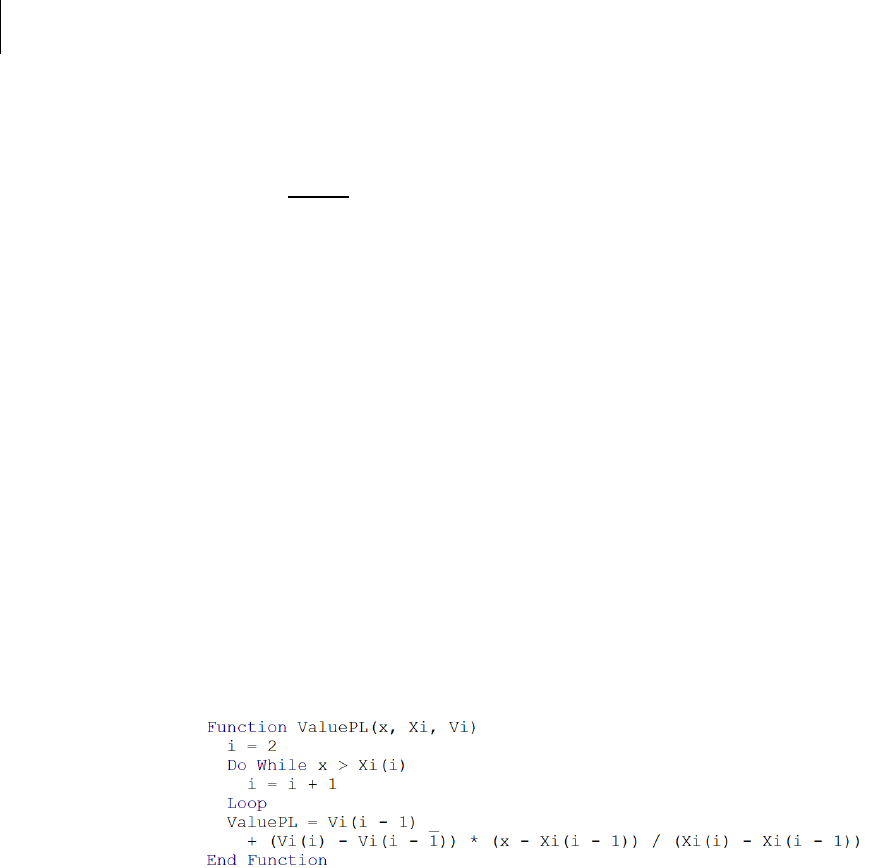
Greg Parnell to illustrate MODA, raw statistics of each player will be evaluated using a macro called

ValuePL, a macro within Excel created by Craig Kirkwood that uses a piecewise linear interpolation. The

essence of this model is captured in the equation below:









  



  

















 

The equation represents the ValuePL for Tyrell Williams’ targets/snap. As seen in Table 2 above, his

0.088 targets/snaps are in between the x values 0 and 0.1 which correspond to the v(x) range of 0 and

60. The ValuePL function then uses the equation above to interpolate between the x and v(x) range to

find his actual v(x), or value, based on the scale that has been defined in the hierarchy. The code iterates

through the possible values of x until it finds that proper range that corresponds with a player’s raw

statistic and then the equation above is performed. The code from the macro can be seen below in

Figure 3 as well.

Figure 3: Code structure of ValuePL function within MODA model.

This process is done for all the value metrics within the value hierarchy and their associated raw player

data. An output for all the processed metrics, or v(x)’s for Tyrell Williams can be seen below in table 3.

Table 3: Example of Player Value Scores V(X)

Player

Snap

Count

Targets/

Snap

Receptions/Target

Yards/Rec

Touchdowns/Rec

Fumbles/Rec

Tyrell

Williams

68.5

52.8

86.3

80.4

58.6

100

The last component of the model is the incorporation of swing weights. Each value metric is

included in a swing weight matrix, with this matrix dependent on 2 categories: the importance of a given

metric and the impact of player variation on this variable. An example of the swing weight matrix from

the model can be seen in Figure 4.

Figure 4: Swing Weight Matrix in MODA Model

As Figure 4 shows, the metrics with the highest f(i), or swing weight values, are those in the category of

“Critical Metric” and “Significant Impact of Player Variation.” The metrics then decrease in swing weight

value, going from “critical metric” to “important metric” across the row and “significant variation” to

“minor variation” down the column. The f(i) value represents the raw swing weight value that a user can

decide upon, and the w(i) represents the normalized swing weight value which is determined by the

individual f(i) value for a metric divided by the sum of all f(i) values. Swing weights are determined by

decision maker preferences, so in the case of this model swing weights were determined by research

Swing Weight Matrix

fi wi fi wi

3. Receptions/Target 65 0.18

1. Total Snap Counts 100 0.28

4. Yards/Reception 55 0.15

2. Targets/Snap 70 0.19 5. Touchdowns/Rec 45 0.13

6. Fumbles/Rec 25 0.07

Significant

impact of Player

Variation

Some impact of

Player variation

Minor impact of

player variation

Critical Metric

Important Metric

sum of fi 360

within the realm of NFL, but decision makers, or general managers, on each team may tend to place

more weight on different metrics than others which will inevitably change the value of swing weights for

these metrics. The swing weights of each metric are then used to weight the (v)x scores for each player’s

individual statistics. An example of the swing weights can be seen in Table 4.

Table 4: Swing Weight for Pre-Determined Value Measures

Snap

Count

Targets/

Snap

Receptions/Target

Yards/Rec

Touchdowns/Rec

Fumbles/Rec

Swing

Weight

0.28

0.19

0.18

0.15

0.13

0.07

Once these swing weights are multiplied by the v(x)’s for a player in each category, the overall value can

be found for a given player by adding up the components of each players w(i)*v(i). Iterating through the

model with Tyrell Williams who is the example above, the overall value can be seen below in Table 5.

Table 5: Total Value Components and Overall Value for Tyrell Williams

Player

Snap

Count

Targets/

Snap

Receptions/

Target

Yards/Rec

Touchdowns/

Rec

Fumbles/Rec

Overall

Value

Tyrell

Williams

19.0

10.3

15.6

12.3

7.3

6.9

2.4 Model Analysis

After the overall value of each player is computed, a value component chart can be created in

order to portray both an individual player’s overall value as well as the components that contribute to

this value. Figure 5 shows the value component chart for Tyrell Williams after iterating through the

model:

Figure 5: Tyrell Williams Value Component Chart

As Figure 5 demonstrates, the length of the whole bar represents the overall value that Tyrell Williams

provides, this being a 71, while the different individual multi-colored sections designate varying metrics

that make up this overall value with the legend for these colors being seen to the right. This type of

chart is extremely valuable to a decision maker because it portrays where a player is collecting value and

where they might be falling behind. As the chart shows, Tyrell Williams collects a high percentage of his

value from total snap counts and receptions/target, but these components are largely determined by

the associated swing weights as discussed. Swing weight variation can have a large impact on the

magnitude of the different components, as will be discussed later in section 2.3.4. While it is valuable to

look at the value component chart for one player, these charts are much more revealing when doing

comparisons among other players to see which categories are ahead and behind similar peers. Figure 6

represents a value component chart for all of the free agents from the 2019-2020 season.

Figure 6: Value component chart for every 2019 free agent for season following free agency

Figure 6 demonstrates the value of each player analyzed in the model broken into the individual

components according to the legend on the right-hand side, allowing the user to see the areas where a

certain player provides more value as well as areas where a player might be lagging behind his peers. It

is important to notice the ideal bar located on the right of Figure 6, with this representing a hypothetical

player who has the maximum value in every value measure. This ideal will be used throughout the rest

of the methodology as a comparison for players. In order to better analyze a general manager’s decision

though, it is important that not only value is incorporated into the decision-making process, but also

salary. Table 6 shows the overall numerical value that a player provides based on this model, as well as

the salary that they were owed during the 2019-2020 season (Sportrac, 2021).

Table 6: Cost and overall value data for 2019 Free Agents

Salary ($M)

Value

Tyrell Williams

11.08

Golden Tate

9.38

Adam Humphries

9.00

Cole Beasley

7.25

Jamison Crowder

9.50

John Brown

9.00

Antonio Brown

10.50

Cordarrelle

Patterson

5.00

Devin Funchess

10.00

Donte Moncrief

4.50

Randall Cobb

5.00

Josh Bellamy

2.50

Andre Roberts

2.30

Chris Conley

2.30

Danny Amendola

4.50

Breshad Perriman

4.00

Michael Crabtree

3.25

Demaryius Thomas

2.91

Allen Hurns

2.50

Seth Roberts

2.00

Tavon Austin

1.75

Dwayne Harris

1.60

Russell Shepard

1.50

Cody Latimer

1.50

Chris Hogan

1.45

Justin Hardy

0.90

Geremy Davis

0.90

Bennie Fowler

0.90

Ryan Grant

0.81

Damiere Byrd

0.72

Marvin Hall

0.65

Conclusions from this data can be better drawn by plotting each players’ overall value vs. their salary,

which can be seen in Figure 7:

Figure 7: Cost vs. Value Chart of 2019 Free agents for season following free agency

The red outline in Figure 7 is seen as the targeted area for a decision maker to look at, that being the

players of low salary and high value. In looking at Figure 7 it is seen that for the free agent class of 2019,

John Brown has the highest overall value at 75 and Chris Conley has the 2

highest value at 74.

However, as the salary vs. value chart shows Chris Conley comes at a $6.6 million discount, something

that must be accounted for by a decision maker in this situation.

2.5 Sensitivity Analysis

Swing weights, as discussed, are an important element of this model and are critical to

establishing a level of importance for each metric. The swing weights that have been decided upon for

this model are discussed above, but there is also sensitivity on these swing weights that can be

examined. Swing weights for each metric can range from a level of 0-100 and these weights can have a

significant impact on a player’s overall value depending on how a metric is weighted. Swing weight

sensitivity can be measured using a dynamic data table as seen in Figure 8:

Figure 8: Data table used for swing weight sensitivity

Figure 8 represents the swing weight values at 0,20,40,60,80 and 100 for the metric fumbles per

reception and the corresponding overall value that occur with these changes. In the model used, this

metric of fumbles per reception was given a value of 25 for the swing weight as discussed, but as the

data table shows a player’s overall value can change significantly based on the decision maker’s

preference on swing weight for this metric. A similar trend of varying overall values can be seen in

looking at the sensitivity of the other metrics as well. The results from the data tables created for each

metric can be looked at by graphing the varying values across the different sensitivity weight values for

each player.

0.00 20.00 40.00 60.00 80.00 100.00

Tyrell Williams 71.41 69.28 71.01 72.55 73.94 75.20 76.34

Golden Tate 69.59 68.23 69.33 70.31 71.20 72.00 72.72

Adam Humphries 60.10 58.33 59.76 61.04 62.19 63.23 64.18

Cole Beasley 70.55 68.36 70.14 71.73 73.16 74.46 75.63

Jamison Crowder 70.90 68.73 70.49 72.06 73.48 74.76 75.92

John Brown 74.81 72.93 74.45 75.81 77.04 78.15 79.15

Antonio Brown 61.72 58.87 61.19 63.26 65.12 66.80 68.32

Cordarrelle Patterson 47.38 43.45 46.64 49.48 52.04 54.35 56.45

Devin Funchess 46.22 42.20 45.46 48.37 50.98 53.35 55.49

Donte Moncrief 40.62 36.19 39.78 42.99 45.88 48.49 50.86

Randall Cobb 67.84 67.07 67.70 68.26 68.76 69.21 69.62

Josh Bellamy 39.65 35.14 38.80 42.06 45.00 47.65 50.05

Andre Roberts 33.25 34.49 33.48 32.59 31.78 31.05 30.39

Chris Conley 73.75 71.79 73.38 74.80 76.07 77.23 78.27

Danny Amendola 64.20 61.53 63.70 65.64 67.38 68.95 70.38

Breshad Perriman 71.46 69.33 71.05 72.60 73.98 75.24 76.38

Michael Crabtree 45.17 41.08 44.40 47.36 50.03 52.44 54.62

Demaryius Thomas 61.14 58.24 60.59 62.70 64.58 66.29 67.84

Allen Hurns 62.15 60.72 61.88 62.91 63.84 64.68 65.44

Seth Roberts 61.77 58.91 61.23 63.30 65.16 66.83 68.36

Tavon Austin 55.80 55.14 55.68 56.16 56.58 56.97 57.32

Dwayne Harris 48.07 44.20 47.34 50.15 52.68 54.96 57.03

Russell Shepard 42.45 38.16 41.64 44.76 47.55 50.08 52.38

Cody Latimer 62.42 59.61 61.89 63.92 65.75 67.40 68.90

Chris Hogan 46.89 42.92 46.14 49.01 51.59 53.93 56.04

Justin Hardy 52.61 49.08 51.94 54.51 56.81 58.89 60.78

Geremy Davis 43.11 38.86 42.31 45.38 48.15 50.65 52.92

Bennie Fowler 54.32 50.91 53.67 56.14 58.36 60.37 62.19

Ryan Grant 39.88 35.39 39.03 42.28 45.21 47.85 50.24

Damiere Byrd 59.04 57.39 58.73 59.93 61.01 61.99 62.87

Marvin Hall 59.45 56.43 58.88 61.07 63.04 64.83 66.44

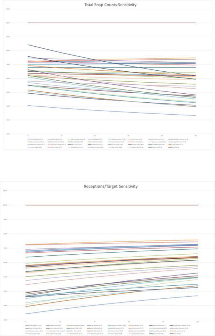
Figure 9: Swing Weight Sensitivity Graph for Total Snap Counts

Figure 10: Swing Weight Sensitivity for Receptions/Target

Figures 9 and 10 represent two extremes for the swing weight sensitivities of the different metrics, with

the “Ideal” on both graphs representing a hypothetical player that has the highest possible value score

for every metric. Figure 10, exhibiting the changes in overall value for each player regarding the

sensitivity of the receptions/target metric is the least volatile of the metrics. Volatility in this case can be

seen as how often the different lines, or players, cross each other. As can be seen, some of the players

do overtake or move below other players, but in general the players overall ranking compared to their

peers are similar for the far-left swing weight value of 0 and the far-right swing weight value of 100. This

can be contrasted with the swing weight graph seen in Figure 9 for the metric total snap counts. As

shown, there is significant volatility in a player’s ranking as the swing weight increases across the chart.

For example, when total snap counts have a swing weight value of 0, the dark blue line representing

Antonio Brown is seen as the player with the highest overall value based on the model computations.

However, as this swing weight value increases, Antonio Brown’s overall value begins to go down

significantly and by the time this swing weight value is 100 he is ranked in the middle of the pack

compared to his peers in this free agency class. These two graphs represent the two extremes of

volatility using sensitivity analysis on the various metrics, with sensitivity volatility of the other metrics

falling in between the metrics for receptions/target(lowest) and total snap counts(highest) and these

can be seen within the appendix.

2.6 Forecasting Using MODA

MODA has many different uses and there are numerous ways of performing analysis on the

results as has been discussed. One interesting way to look at the results is to look at a common group of

players and use the previous year’s data to see how well it predicts the overall value of a player in the

next year. This was performed using the set group of wide receivers that has been discussed throughout

the rest of the methodology, the 2019-2020 free agent class. 2018-2019 data, the year before the

groups’ free agency, was used and compared to the 2019-2020 data and results that has been previously

discussed. Figure 11 shows the results of this process, with 2018 being the data set acting as the

predictor and 2019 being the other year in the comparison. The percent difference from this was also

calculated for each player year over year which can also be seen in Figure 11 as well.

Figure 11: Comparison of Percent Error for Value Year over Year and variation in metrics

As Figure 11 demonstrates, for some of the players such as Marvin Hall, Danny Amendola, and Tyrell

Williams the data from 2018 does an excellent job of predicting the performance of these players for the

next year, with % differences of 1% each. However, some of the players have very high % differences

with some players seeing over 20% differentials year over year. In looking at some of the possible

reasons for these large differentials, it became clear that snap count variation had a huge impact on the

overall value variation. The percent change for all metrics was calculated year over year, with the

exception of touchdowns and fumbles since these values are 0 for many players, and it can be seen that

the players with the highest value differential also saw the highest impacts from snap count variation on

average. Snap counts can vary widely based on a specific player mainly due to injuries, but also a

number of other qualitative factors as well. The effect of snap count variation can be seen in Figure 12:

Figure 12: Overall Value % Change vs. Snap Count % Change 2018 vs. 2019

50%

100%

150%

200%

250%

0% 20% 40% 60% 80% 100%

Snap Count % Change

Overall Value % Change

Overall Value % Change vs. Snap Count % Change

2018 vs. 2019

This graph demonstrates that players that saw a relatively low snap count percentage change also had a

relatively low overall value % change. This indicates that, based on this sample of players, when a player

receives the same amount of snap counts year over year the model does a good job of predicting future

value for a certain player. When high snap count variation happens though, the model is not as precise

in predicting the future value as the player’s opportunities to collect value is limited. While not much

can be done about this in the current model, this limitation will be further expanded in the next section.

3. Future Improvements

As discussed throughout the methodology, there are numerous ways to analyze and interpret

the results of the MODA process in the context of NFL players in a position group. MODA is not a

methodology that has been used much at all in the context of the NFL, and as this research has shown it

demonstrates some very promising results. With this being said, there is still plenty of space for future

development on this work to improve model accuracy and advance the methodology as a whole.

The metrics that were chosen on this research were based on widely used statistics that have

been shown by experts to be very important to measuring a player’s success on the field. However,

changing or adding to these statistics may prove to further increase the accuracy or validity of the model

for wide receivers. This model is purely focused on on-the-field statistics, but to get a wholistic view of a

player it may be important to a decision maker to incorporate many more types of factors such as age,

physical measurables, and aspects such as injury or off-the-field incidents. Another aspect of this specific

application of MODA that may be improved upon is using many years of data to look at how the results

hold up over time. In the methodology, the results of MODA were compared year over year to see how

well the model acted as a predictor for the next year. This can be further expanded by looking at a

player’s statistics over the course of several years, not just one year, to see its accuracy over a longer

period of time.

This paper also only shows the effects of MODA for one position group, wide receivers. While

the statistics that are being incorporated in the model will change for differing position groups, the

methodology will stay the same leaving room for this model to be applied to a variety of position groups

on which a general manager will need to make decisions. Another application of this model can be

deciding the allocation of money for different position groups as a whole. This research is for making

player to player comparisons within a specific position group, but it can also be used to develop a

hierarchy for fund allocation for different position groups on an entire team based on a decision maker’s

preferences.

Appendix:

Table representing data used in MODA model for each player from 2019-2020 season

Figure of Target/Snap Count Sensitivity

Figure of Yards/Reception Sensitivity

Figure of Touchdowns/Reception Sensitivity

Figure of Fumbles/Reception Sensitivity

References

Dadelo, S., Turskis, Z., Zavadskas, E. K., & Dadeliene, R. (2014). Multi-criteria assessment and ranking

system of sport team formation based on objective-measured values of criteria set. Expert

Systems with Applications, 6106-6113.

Deehr, J. (2017, August 28). Multi Objective Decision Analysis in R. Retrieved from https://rstudio-pubs-

static.s3.amazonaws.com/300421_0e5019919ff146ab9d16e27b09fbf767.html

Gaines, C. (2014, September 18). Look How Much More Quarterbacks Are Paid Than Everyone Else.

Retrieved from Business Insider: https://www.businessinsider.com/nfl-highest-paid-positions-

2014-9

Hernandez, T. (2018, July 31). The Most Predictable Wide Receiver Stats. Retrieved from Sports

Illustrated: https://www.si.com/nfl/2018/07/31/fantasy-football-2018-most-predictable-wide-

receiver-stats

HowMuch. (2016, July 1). Which Professional Sports Leagues Make the Most Money? (howmuch)

Retrieved 2020, from https://howmuch.net/articles/sports-leagues-by-revenue

Jones, K. (2019, January 20). NFL Television Ratings Rose 5% in 2018. Retrieved from Sports Illustrated:

https://www.si.com/nfl/2019/01/03/nfl-television-ratings-viewership-rise-five-percent-2018

Lineups. (2021). 2020 NFL Snap Counts (Live Update). Retrieved from Lineups:

https://www.lineups.com/nfl/snap-counts

Porter, J. (2018). Predictive Analytics for Fantasy Football: Predicting Player Performance Across the NFL.

University of New Hampshire Scholars Repository.

Pro Football Reference. (2020). 2019 NFL Receiving. Retrieved from Pro Football Reference:

https://www.pro-football-reference.com/years/2019/receiving.htm

Sportrac. (2021). 2019 NFL Free Agents. Retrieved from Sportrac: https://www.spotrac.com/nfl/free-

agents/2019/wide-receiver/

Tani, S. N., Johnson, E. R., Parnell, G. S., & Bresnick , T. (2013). Handbook of Decision Analysis .