Price Performance in the CAISO's Energy Markets

MQCRA/MA&F/GBA 1

Price Performance in the CAISO’s Energy

Markets

June 18, 2019

Prepared by:

Market Analysis and Forecasting

California Independent System Operator

MQCRA/MA&F/GBA 2

MQCRA/MA&F/GBA     3 
 
Table of Contents 
 
Acronyms ...................................................................................................................................................... 4 
Background and Scope .................................................................................................................................. 5 
Responses to Stakeholders Comments ......................................................................................................... 6 
Market Structure and Price Performance ..................................................................................................... 9 
Gas-Electric Price Dynamics ........................................................................................................................ 23 
Load Adjustments ....................................................................................................................................... 26 
Load and Market Requirements ................................................................................................................. 32 
Exceptional Dispatches ............................................................................................................................... 46 
Detailed Analysis of Price Performance ...................................................................................................... 49 
Price divergence in July 2018 .................................................................................................................. 49 
Price divergence on March 1, 2018 ........................................................................................................ 61 
Price divergence on September 5, 2017 ................................................................................................. 62 
Price divergence in March 1, 2019 ......................................................................................................... 62 
Price divergence in June 19, 2017 ........................................................................................................... 64 
Price divergence in March 3, 2019 ......................................................................................................... 64 
Scheduling of VER resources in IFM ........................................................................................................ 65 
RUC adjustment for day-ahead market of July 8, 2018. ......................................................................... 66 
Marginal Units ............................................................................................................................................. 69 
Proposed Plan for Analysis .......................................................................................................................... 73 
Scope of analysis ..................................................................................................................................... 73 
Stages of analysis .................................................................................................................................... 74 
Proposed schedule ...................................................................................................................................... 75 
Appendix ..................................................................................................................................................... 76 
 
   

MQCRA/MA&F/GBA 4

Acronyms

BAA

Balancing authority area

Convergence bid

DAM

Day-ahead market

DOT

Dispatch operating target

Exceptional dispatch

EIM

Energy imbalance market

FMM

Fifteen-minute market

HASP

Hour ahead scheduling pre-dispatch

IFM

Integrated forward market

LMP

Locational marginal price

MCC

Marginal congestion component

MLC

Marginal Losses component

RTD

Real-time dispatch

RUC

Residual unit commitment

SMEC

System marginal energy component

VER

Variable energy resource

MQCRA/MA&F/GBA 5

Background and Scope

In early 2019, the CAISO committed to analyze price formation in its electricity markets. In this context,

the term price formation refers to the underlying principles that define the electricity prices under

locational marginal pricing. The Federal Energy Regulatory Commission (FERC) launched a price formation

effort in 2014 to address areas such as scarcity and shortage pricing, fast-start resource pricing, offer bids

and caps, among others

. The California ISO, like other ISOs and RTOs, actively participated in each of

these initiatives. The analysis in this effort focuses more narrowly on price performance across the CAISO’s

markets.

CAISO stakeholders have raised concerns about i) whether real-time prices adequately reflect constrained

system conditions, ii) the fact that real-time prices have trended lower than day-ahead prices, and iii)

concerns about the market rules for intertie energy deviation settlements, which are documented in the

CAISO Market Surveillance Committee opinions

The goal of this effort is to identify and analyze the dynamics and drivers of price performance across the

CAISO’s markets. Based on feedback from participants, the analysis will use a longer timeframe, spanning

from January 2017 to March 2019 so that it is extensive enough to account for seasonal variations as well

as to capture the trends over a longer horizon. In addition, the analysis will only look into the real-time

market for the CAISO balancing area. However, the results may prove relevant to the EIM balancing

authority areas as well.

The outcome of this analysis will inform potential action items to address identified price performance

issues. Throughout this effort, there will be opportunities for market participants to engage and provide

feedback and suggestions about direction for further analysis. IF needed, the CAISO will refine the scope

of its analysis.

As scheduled in the original plan, this report provides market participants an update on the progress of

the analysis and solicits feedback on the direction the CAISO should continue to work. All metrics

presented in this partial update are subject to further validation and adjustment.

FERC initiative on price formation can be found at

https://www.ferc.gov/industries/electric/indus-act/rto/energy-price-formation.asp

MSC Opinion Intertie Deviation Settlement: http://www.caiso.com/Documents/MSC-

OpiniononIntertieDeviationSettlment-Jan18_2019.pdf#search=MSC%20intertie

MQCRA/MA&F/GBA 6

Responses to Stakeholders Comments

When the ISO committed to launch this analysis effort, stakeholders expressed interest in actively

participating and helping set the direction of the analysis to address specific concerns regarding price

performance. In order to accommodate this interest, the ISO organized this analysis effort in such a

manner to allow engagement and feedback from participants as the ISO progresses on this analysis.

The ISO appreciates stakeholder comments in response to the proposal for analysis of price performance.

The ISO posted a white paper on April 3, 2019 and held a conference call on April 10, 2019 to discuss the

scope and schedule of this analysis effort. Previously, the ISO discussed this analysis effort in the Market

Surveillance Committee (MSC) session of April 5, 2019. The ISO received 12 sets of comments

Calpine suggested complementing the analysis with an evaluation of bid cost recovery as a vehicle to

identify potential drivers of price performance. The ISO will consider this item for potential analysis.

Calpine seconded the questions raised by the MSC in their opinion about the Intertie Decline effort to

analyze flexible ramp product performance and the manual intertie dispatches. These two areas are

within the scope of this analysis. Calpine similarly requested the ISO to select specific days with

problematic price performance and rerun the market under a perfect dispatch construct in which all actual

conditions are used. In this regard, this concept of perfect dispatch may naturally apply to an ex-post

market that relies on actual conditions to come with prices. In contrast, the ISO uses an ex-ante construct

in which the market clears and the prices are set based on projected conditions. This makes a rerun of a

counterfactual dispatch using actual conditions more problematic. In the RTM, where the current solution

heavily depends on the previous solution, changing one condition in a given interval will change not only

the market outcome of that interval but the setup and market solution for any subsequent market,

effectively creating a parallel world of market solutions. For the scope of this specific analysis effort, the

current ISO technology is not setup to be able to create a counterfactual market that can accurately

internalize the actual conditions. The ISO still sees merit with the overall concept of having specific cases

rerun with some changes included to realize the effect of that change, such as the inclusion of operator

actions.

The California Large Energy Consumers Association (CLECA) suggested adding the impact of Reliability

Demand Response Resources (RDRR) to the price performance scope. Based on historical outcomes, RDRR

are only dispatched in the real-time market once the ISO system is in or is eminently getting into a system

emergency. These instances are infrequent and isolated and, thus, RDRR performance is not a primary

driver of the more recurrent price performance concerns. The ISO will consider this suggestion as a

potential item in the analysis.

Pacific Corporation (PAC) seeks clarification regarding the intended actions to be taken from the outcome

of this effort. This ISO notes that this is an analysis effort and not a policy effort. The ISO envisions that

this analysis effort can shed light into the drivers of price performance issues; these drivers, in turn, may

The straw proposal and as well as the stakeholder comments are available at

http://www.caiso.com/Pages/documentsbygroup.aspx?GroupID=6C9CDFDA-E9A0-4F65-9FC6-4CB01C1ADAA5

MQCRA/MA&F/GBA 7

point to different levels of next actions. There could be actions as simple as correcting identified defects

or gaps in the implementation of certain market functionality, identifying areas for potential

enhancements in the existing market functionality, or creating inputs for further policy evaluation

regarding market design. PAC supported the scope of the analysis, including operator actions as a whole,

and highlighted the role that integration of renewable resources may play in price performance. Lastly,

PAC put in context a broader discussion of the design of extended day-ahead market and the ongoing day-

ahead market enhancements. This analysis effort is not a substitute to any policy initiative but may instead

actually provide inputs and information to better guide these policy discussions.

Powerex indicated that the price formation issues discussed in the proposal have their origin in the design

of having an energy-only market, which creates a misalignment between the CAISO market and the actual

needs of the grid, and urged the ISO to consider this from a more underlying market design angle. Powerex

elaborated on their guiding principles by advocating for a more efficient market. They provided a white

paper on efficient markets (dated March 2019) which is perhaps more in the context of recent discussions

of the CAISO DAM enhancements. The white paper notes that rapid changes in the resource mix may be

exposing the CAISO’s limitations of the energy-only market. The ISO notes that the expected scope of this

effort is more on the evaluation of the existing and current market design, and not about exploration of

alternative market design. There are other efforts in the policy spectrum that may be better place to

discuss policy design. This analysis effort naturally might provide inputs to policy discussions such as the

ongoing DAME policy.

PG&E suggested focusing the analysis on how each contributing factors impacts price performance and

to what extent. It also suggested rerunning counterfactual cases to compare the effect of operator

actions. As part of this analysis, the ISO expects to cover these suggestions. NRG suggested making all data

available, while PG&E suggested releasing load conformance and exceptional dispatch data. The ISO will

consider these suggestions. Changes to existing applications to publish data, either publicly or through

participants portal, require system changes.

NRG and SCE suggested expanding the analysis period beyond the originally proposed period of 2018. The

ISO has considered this suggestion, and will expand the analysis period to cover 2017 through the first

quarter of 2019. This will allow for a longer period of analysis while still being recent enough to ensure

drivers are still relevant. Additionally, this period will cover the peak days of September 1, 2017, July 25

2018 and March 31, 2019 which are useful as peak days tend to demonstrate unusual conditions that

“stress test” the markets. NRG also suggested that this effort go one level deeper in analyzing the impact

of market operator actions on price performance. The ISO expects to be able to analyze the impact of the

various operator actions on the price performance. NRG also suggested that the ISO use case studies to

provide detailed analysis of price performance issues. This type of analysis is within the scope of this effort

and, in this partial update, the ISO is providing some cases studies already analyzed in response to this

suggestion.

SCE suggested analyzing the potential impact of load forecast accuracy, virtual bids, and gas-related

drivers since these factors can have an impact on price performance. For instance, load forecast errors

can influence the procurement of ancillary services. These items are all within the scope of this analysis

effort. SCE suggested allowing stakeholders to submit comments after the release of the first report. The

MQCRA/MA&F/GBA 8

ISO has adjusted the schedule to include a time window during which participants can review the report

and submit comments. Depending on the extent of these comments and their potential to trigger changes

in the scope of the analysis, this may impact the suggested analysis completion date.

Seattle City Light (SCL) generally supported the ISO’s suggested scope and suggested using counterfactual

cases (reruns) to analyze the effect of certain market aspects such as the inclusion of virtual bids. The

ongoing analysis effort is doing this type of analysis. Furthermore, SCL suggested expanding the analysis

to explore implications of having an energy-only market and this situation’s interplay with firm energy.

The ISO notes that expected scope of this effort is more on the evaluation of the existing and current

market design; there are other efforts in the policy spectrum that may be better place to discuss policy

design. This analysis effort may provide inputs to policy discussion such as the ongoing DAME policy. SCL

also suggests that this effort should become a regular and recurrent effort and evaluation. Based on the

outcome of this effort, the ISO may evaluate if there is any need beyond this scheduled deliverable.

Shell suggested including analysis on price formation at the interties as well as analysis based on

counterfactual market outcomes and very specific market cases. The ISO notes that this ongoing effort is

explicitly looking at the performance of interties and also uses case studies based on counterfactual

solutions. Some of these results are provided in this partial report.

The cities of Anaheim, Azusa, Banning, Colton, Pasadena, and Riverside, California (“Six Cities”) suggested

comparing the frequency and magnitude of price divergence with other ISOs’ markets. The ISO will search

for such metrics to see if they are readily available for comparison but, given the tight schedule for this

analysis, the ISO may not commit to do any direct comparisons with other ISOs’ markets.

WPTF generally supported the proposed scope and encouraged the ISO to connect this effort with other

policy discussions such as the enhancements for the DAM. It also encouraged the ISO to re-visit the

schedule if needed to produce a comprehensive study, and to consider the importance of transparency

for a well-functioning market. It suggested also analyzing the transmission differences. The ISO notes that

this area has not been envisioned within the original scope of analysis, although is a critical component in

the proper functioning of the LMP-based markets. The ISO proposes to continue working on the original

scope and consider a potential second effort to target transmission- and congestion-related efforts.

MQCRA/MA&F/GBA 9

Market Structure and Price Performance

Based on the CAISO market design for the Day-Ahead Market (DAM) and the Real-Time Market (RTM),

prices between these markets are expected to converge to a reasonable degree, subject to changes in

system conditions. The level of price convergence across markets, and the degree to which prices reflect

actual system conditions are natural indicators of robust price performance in the CAISO markets.

The RTM is composed of three sequential sub-markets that are run at different times, granularities, and

forward looking horizons. There is a fifteen-minute market (FMM), in which both internal generation and

intertie resources can be economically cleared based on submitted bids. The outcome of this market is

financially binding for both internal and intertie resources. The FMM runs for a horizon of up to four and

a half hours ahead and as short as one hour ahead, and runs approximately 37.5 minutes ahead of the

binding interval. For intertie resources participating on an hourly basis, the financially binding schedules

are determined in the hour ahead scheduling process (HASP) instead of the FMM. However, the FMM

clearing prices are used to settle hourly resources. For internal resources, the FMM schedules are

financially binding, but they do not set physical operational instructions for energy because they are

ultimately subject to the five-minute real-time dispatch (RTD). FMM commitment instructions -start-ups,

shutdowns and transitions- are, however, physically and financially binding. In the RTD market, both

dispatches and prices are operationally and financially binding. The RTD runs for a horizon of up to one

hour and five minutes and runs 7.5 minutes ahead of the binding interval. The CAISO follows a standard

multi-step settlements process, in which the DAM is settled fully and subsequent markets are settled

incrementally, i.e., FMM schedules settle with respect to the integrated forward market (IFM) awards,

and RTD settles with respect to those in the FMM. The CAISO settles the volumetric difference of hourly

schedules relative to IFM schedules, based on FMM prices. When prices diverge persistently across the

multi-step settlements, resources could arbitrage across markets. Convergence bidding is intended, in

part, to help converge prices between the DAM and RTM.

Prices in the CAISO market consist of three main components – the system marginal energy cost (SMEC),

the marginal congestion cost (MCC), and the marginal cost of losses (MCL). The SMEC reflects the marginal

cost of meeting the system-wide demand. The MCC is based on the binding transmission constraints in

the system and varies by location. The MCL reflects the sensitivity of a location to system losses. Price

performance, such as convergence, at the system level can be measured using the SMEC, which will

illustrate price convergence to meet system-wide supply and demand. Although the price decomposition

of locational marginal prices is relative to the selection of the slack node, the SMEC can generally provide

a reasonable reference of the power balance (supply equals demand) at the system level.

Another option is to rely on a different construct that is independent of the slack selection, in this case

taking the full locational marginal prices. Typically, Default Load Aggregation Points (DLAP) or Trading

Hubs (THs) have been used as a reference. In this report, a reference price is constructed by taking a

weighted average of the four DLAPs in the CAISO system, namely, DLAP_PG&E, DLAP_SCE, DLAP_SDG&E

and DLAP_VEA. The weights are the amount of load cleared at each DLAP. Such price will be called system-

MQCRA/MA&F/GBA 10

weighted price. The difference between the SMEC price and the system-weighted price will reflect the

marginal losses and congestion observed at the DLAP level.

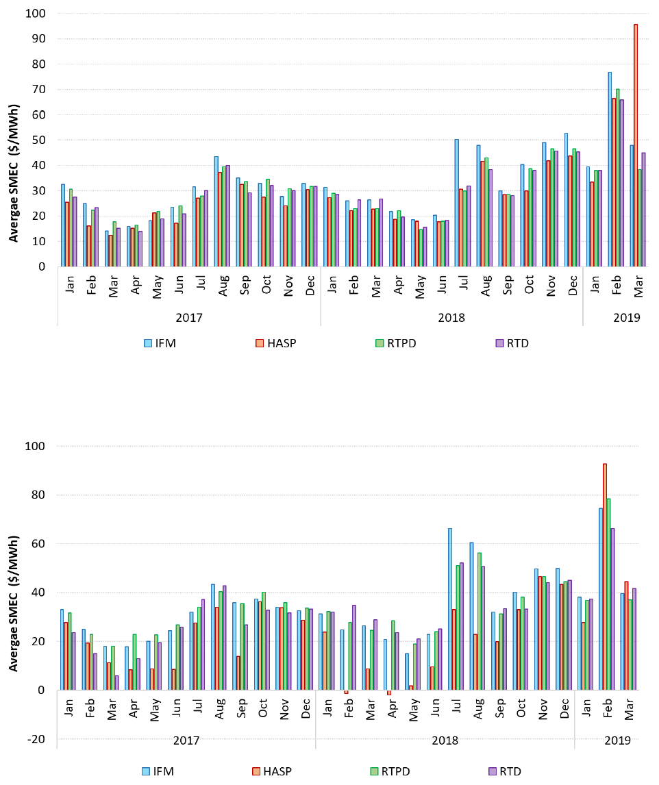
Figure 1 through Figure 4 show the simple averages of system weighted prices compared across the

various CAISO markets

. Figure 1 shows a monthly trend, while Figures 2 through 4 show the averages on

an hourly profile broken out by calendar year. Overall, IFM prices in 2018 tended to be higher than real-

time prices for most times of the day, with the largest divergence observed in the summer months. Within

the various runs of the real-time market, the trend of price divergence is less pronounced and has a less

persistent trend as compared to the IFM. The Appendix shows the same metrics using instead the SMEC

component only. In comparison to the statistics with the weighted average price, those based on SMEC

prices and presented in the Appendix show similar trends of price convergence, even though some

months generally show a larger divergence using SMECs. The monthly trend also shows an interesting

factor of the market dynamic fairly influenced by the gas-system dynamic. Months like July 2018, or

February and March 2019 are a reflection of higher and more volatile gas conditions. With the ISO market

relaying fairly on gas resources, the electric prices –either SMEC or DLAPs- will move accordingly, with

higher electric prices when gas prices increased.

Figure 1: Monthly comparison of average system- weighted prices across the CAISO markets

Figure 2 illustrates the price convergence on an hourly profile, which shows that IFM prices are

persistently higher than real-time prices starting in 2018 and continue in 2019. This divergence is more

pronounced during peak hours when the system is naturally tighter in supply. As discussed in subsequent

All prices in IFM, FMM and RTD are financially binding, i.e., they are validated and corrected when necessary.

However, the HASP pries are not financially binding, and they are not corrected after the fact. The IFM, FMM and

RTD prices used in this analysis are the financially binding, validated and corrected prices, but the HASP prices are

the original prices produced by the HASP market and do not reflect any price corrections.

MQCRA/MA&F/GBA 11

sections, the CAISO markets are experiencing the highest prices not during the gross peak hours but more

pronounced during the hours of the net load peak.

Figure 2: 2017 hourly comparison of average system-weighed prices across the CAISO markets

Figure 3: 2018 hourly comparison of average system-weighted prices across the CAISO markets

MQCRA/MA&F/GBA 12

Figure 4: 2019 hourly comparison of average system-wide prices across the CAISO markets

Either SMEC or the system weighed price can provide an accurate reference of price performance at the

system level. However, the price performance at scheduling points of interties may be different from a

system-based performance. This is because there may be specific design features in the CAISO markets

related to the treatment of interties, which may lead to congestion differences among markets that

metrics on either SMEC or DLAPs will not capture explicitly. As part of this analysis, the ISO is also

investigating the price performance on interties. Figure 5 through Figure 7 illustrate price convergence at

representative scheduling points for the interties of Malin, NOB and Paloverde. These three interties are

taken as a proxy reference for intertie performance since they are the main interties at which a significant

volume of energy is traded in the CAISO system.

Although HASP prices are not used to financially settle interties, this market produces financially binding

schedules for hourly intertie, which are then settled at the FMM prices. Intertie resources can participate

in the CAISO markets under different formats. They can opt to use i) hourly interties, which means they

are scheduled with a flat hourly profile in the HASP market; ii) fifteen-minute resources what are

scheduled in FMM on fifteen-minute basis, and for which their schedule may vary from interval to interval

in the hour; and iii) one-time adjustments, which allows resources to make an adjustments to their hourly

schedule through the FMM. Regardless of these scheduling options, intertie schedules are all settled

based on the FMM prices. Hourly interties are by large the main type of interties participating in the CAISO

markets. Thus, divergence between HASP and FMM prices have direct implications in the real-time

markets. Both Paloverde and Malin interties reflect similar trends to the system weighed prices during

some of the most pronounced periods, such as the summer of 2018 when IFM prices were fairly higher

than real-time prices. However, NOB intertie particularly shows a more pronounced divergence mainly at

MQCRA/MA&F/GBA 13

the HASP market. Generally, NOB intertie has observed fairly lower prices in HASP relative to the other

markets.

Figure 5: Monthly average LMP at Malin scheduling point

Figure 6: Monthly average LMP at NOB scheduling point

MQCRA/MA&F/GBA 14

Figure 7: Monthly average LMP at Palo Verde scheduling point

Although averages can provide a rough visualization of how prices may be evolving overtime, they are too

coarse to capture the frequency and magnitude of the price spreads across markets. Figure 8 through

Figure 11 show the price distribution of each market using box-whisker plots. The boxes stand for the 10

and 90

percentile, the whisker stand for the samples between the minimum value and the 10

percentile, and from the 90

percentile to the maximum value. The blue marker in the box stands for the

median (50

percentile), while the red marker stands for the simple average price. In order to graphically

show a meaningful level of prices, these figures have been limited to a price range between -$50/MWh

and $150/MWh. The plots with a full price range are shown in Figure 84 through Figure 87 in the Appendix.

There are certain months in which the price variation increased largely, these happened in the months of

July, and August 2018 when peaking conditions occurred in the system combined with high gas prices,

and also in February and March 2019 when volatile gas conditions were observed in the west. In these

months, 80 percent of the prices move in a range of $90/MWh, in comparison to the price window of

$35/MWh observed in other months.

MQCRA/MA&F/GBA 15

Figure 8: Monthly prices in IFM

Figure 9: Monthly price in HASP

MQCRA/MA&F/GBA 16

Figure 10: Monthly prices in FMM

Figure 11: Monthly prices in RTD

MQCRA/MA&F/GBA 17

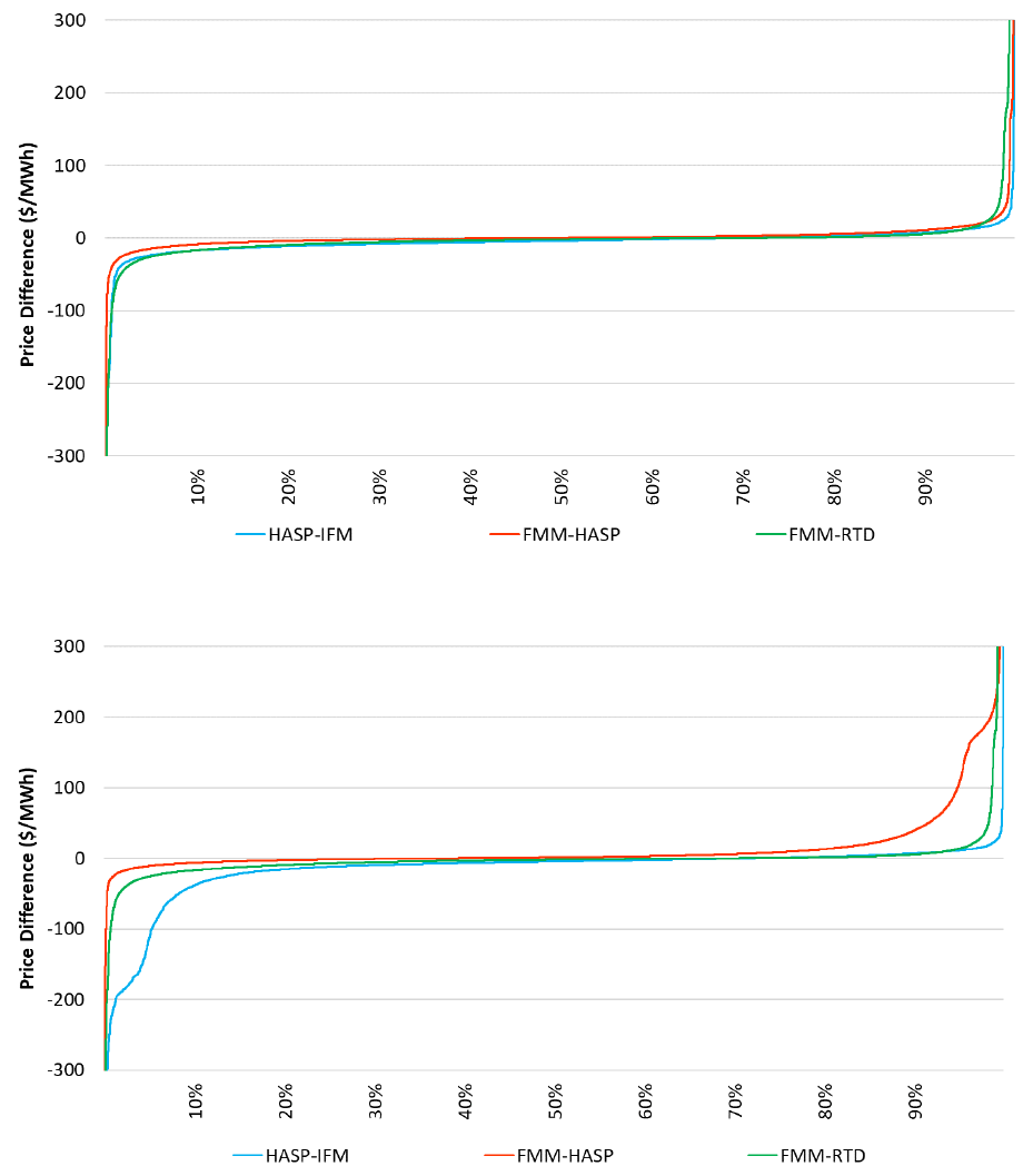
Figure 12 through Figure 14 show the distribution of price between two CAISO markets; these spreads

are calculated with the system-weighted average prices from DLAPs

Figure 12: Price spreads between IFM and HASP

Figure 13: Price spreads between HASP and FMM

The spreads are calculated as (HASP-IFM), (FMM-HASP) and (RTD-FMM).

MQCRA/MA&F/GBA 18

Figure 14: Price spreads between FMM and RTD

In order to see a meaningful trend, these plots narrow the display in a range of ±$60/MWh. The largest

spread are observed between the IFM and HASP markets, and more pronounced in the months of July

2018 and February 2019. The HASP-IFM spread are more concentrated in the negative range, which

indicates a higher frequency of price divergence between these two markets is when IFM prices are higher

than HASP prices. This is the same pattern observed with simple averages introduced in earlier metrics.

Across the months, FMM-HASP spreads are more evenly distributed, which would reflect a better

performance than HASP-IFM spreads. These spreads also show that the simple averages may not be as

reflective to measure price convergence. For the RTD-FMM spreads, a larger volume is concentrated in

the negative range, which indicates that a higher frequency of spreads show higher prices in FMM, while

the simple averages may also not properly show the price dynamic.

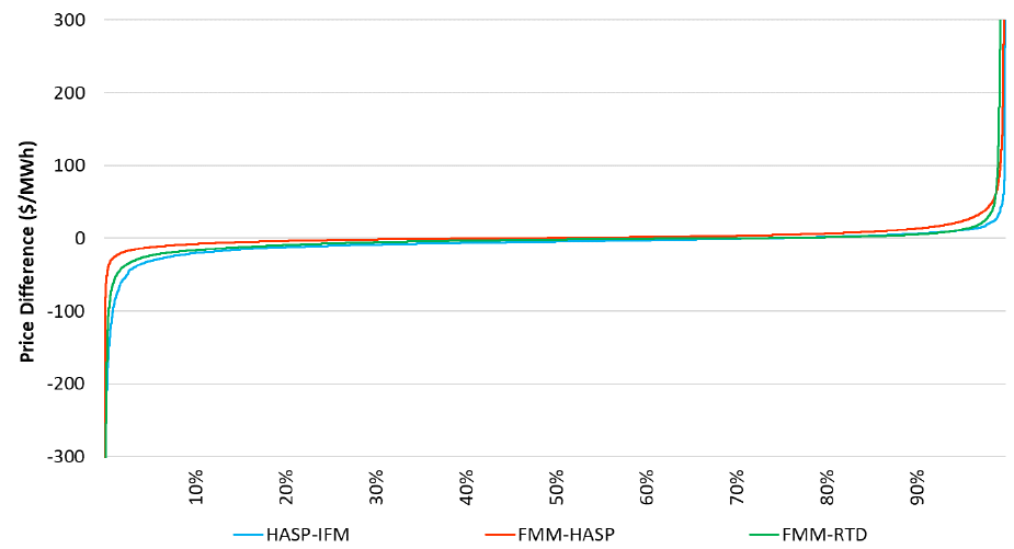
Figure 15 shows a simple correlation plot for the price spreads between markets. A large volume of the

spreads is concentrated in the low-price range, and as the spreads become larger the correlation is

weaker, with price spreads largely scatter mainly in the positive quadrant of the price spreads. This is

significant in the RTD-FMM spreads. Some price spreads can reach a $1000/MWh and typically may

happen when the price in one market spikes to the scarcity point while the price in the other market stays

low or even negative.

MQCRA/MA&F/GBA 19

Figure 15: Price correlation between CAISO markets

In addition to the magnitude, the frequency of price divergence conveys important information. Figure 16

shows the frequency when the price in one market is higher than the price in other market used in the

spread calculation. Under this metric, prices are compared side to side between markets for each

interval

. For instance, the hourly price observed in a given hour of the IFM is compared against the hourly

price of the HASP market. Similarly, the hourly price in the HASP market is compared against the four

prices of its according four intervals of FMM. For the correlation between FMM and RTD markets, there

is a marked area of divergence along the y axis, these points reflect instances where the FMM prices is

within normal price range, but RTD prices are all the way up to $1000/MWh. This is expected to some

extend because the RTD market may experience temporary ramping constraints, which typically arise due

In order to avoid very small price differences distorting the metric, price difference within 25 cents –positive or

negative- are not included in this metric.

MQCRA/MA&F/GBA 20

to the inherent changing conditions in the RTD market. This condition is not that pervasive in the other

markets, which are optimized over longer periods (fifteen or hourly), because those markets’ running

horizon can absorb the ramping and changing conditions and they are exposed to less volatile conditions.

For example, in July 2018, the bar in blue stands for the price divergence between IFM and HASP market

and is about 80 percent. This means that about 80 percent of the time (hours) in that month, the price in

IFM was higher than the price of the HASP market. For the bar in red, it indicates that about 50 percent

of the FMM intervals in that month the prices in the HASP market were higher than the prices observed

in FMM.

Figure 16: Monthly frequency of price divergence between markets

When analyzing frequencies, it is expected to see frequencies of about 50 percent, which would mean a

half of the time prices in one market are higher than prices in the other market. This would indicate normal

distribution of price spreads. Values much different than 50 percent would simply mean that there is a

more systemic and persistent price divergence between markets. For the period under analysis,

frequency-wise the price differences between HASP and FMM are evenly distributed as each month is

about 50 percent. This is not the case for the price differences between IFM and HASP and FMM and RTD,

which observed frequencies of about 64 to 61 percent, and in some specific months this frequency was

as high as 80 percent. This frequency alone still does not provide a meaningful reference about the

magnitude of such price divergence. However, it may highlight how pervasive the price divergence may

be.

Regarding interties, similar frequency of price divergence is illustrated with a duration curve in Figure 17

through

MQCRA/MA&F/GBA 21

Figure 19 for the year of 2018. For Malin and Palo Verde, such curves illustrate that the price spreads are

more evenly distributed between positive and negative spreads. However, NOB intertie shows a

significant divergence between markets, mainly driven by prices in the HASP market. To fully understand

the drivers of this divergence, some specific intervals were taken for a detailed analysis; that analysis is

introduced in subsequent sections.

Figure 17: Duration curve for prices at Malin scheduling point

Figure 18: Duration curve for prices at NOB scheduling point

MQCRA/MA&F/GBA 22

Figure 19: Duration curve for prices at Palo Verde scheduling point

MQCRA/MA&F/GBA 23

Gas-Electric Price Dynamics

Currently, the ISO relies on gas prices to calculate caps on commitment costs and default energy bids. For

resources using proxy-cost option for commitment costs, the ISO uses next-day gas prices from up to three

vendors (NG, Platts and SNL). The ISO uses the gas indices for the hubs SoCal City gate, PG&E Citygate,

and Kern River delivery pool. These gas indices with transportation costs and other miscellaneous costs,

are used to calculated different fuel region prices, which in turn are used to estimate the commitment

costs and DEB. This calculation is done daily and overnight, so that it can be used for the real-time market

for next trading date. Without the Aliso Canyon provisions, this same index would be used for DAM as

well that is run next morning for the subsequent trading date. For the DAM and under the Aliso Canyon

provisions, the ISO takes every morning, when gas trades occur, the estimated weighted average price

from the Intercontinental Exchange (ICE) and replaces the previous night calculated index as described

above. In this way, the DAM runs with the most recent price trends because the one day lag is eliminated.

For weekends and holidays, when there are no gas trades on ICE, the system falls back to use the most

recent index available which is the index calculated the previous night. Note that the variable cost for gas

resources can be bid directly by market participants and cap to $1000/MWh. If any resource is mitigated

as part of the market power process, its variable-energy bids will be mitigated to the highest of the

competitive locational marginal price or the DEB.

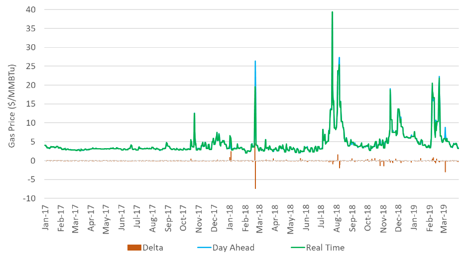
Figure 20: Trend of gas prices between the day-ahead and real-time markets

Figure 20 shows the comparison of the commodity price used for SoCal resources, which is derived from

the So Cal city gas hub. For RTM, it reflects the blended index from the gas prices available from the

various vendors; for DAM, it reflects the estimated ICE weighted price obtained in the morning just prior

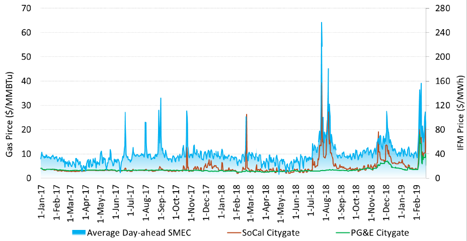
MQCRA/MA&F/GBA 24

to the DAM. These prices also reflects any price that may have been applied by using the internal ISO

fallback logic, when for any reason the gas price for next day was not available. As expected, the majority

of time the day-ahead price tracks closely the real-time price given the manual update that takes place

every morning and that has helped to eliminate the additional one-day lag. There is a relative small set of

days with divergence in gas prices between the day-ahead and real-time markets, as shown by the bars

in red. This is observed when there is volatility in the gas market.

There are two main aspects where gas dynamics can lead to an electric price divergence. First, bids will

reflect the gas prices difference in the DAM and RTM and drive the clearing prices in the electric market.

In other words if gas prices are higher in the RTM, commitment costs and DEBs will reflect these higher

prices. Secondly, bids will internalize the price differentials, and thus the bids clearing the RTM may be

priced accordingly to the higher gas prices. Thus, even if the same supply is bid in real time, it may come

at higher bid prices. Consequently, either commitment costs, DEBs or variable energy bids may drive the

market clearing prices and the price divergence between markets.

Figure 21: Trend of gas and electric prices in the day-ahead market

Figure 21 shows both gas and electric prices for the day-ahead timeframe for the period under analysis.

For gas prices, the PG&E and SoCal city gates hub prices are shown, since these are the two main hubs

used to define the fuel regions in the CISO markets. There is a strong influence of gas prices in the electric

prices. For the period of analysis, there was gas price volatility in the SoCal region that directly translated

into the electric prices. Figure 22 shows a strong correlation between gas and electric prices in all ranges

of prices. The electric prices are simple daily average prices in order to march the daily nature of the gas

prices.

MQCRA/MA&F/GBA 25

Figure 22: Correlation of gas and electric prices in day-ahead market

MQCRA/MA&F/GBA 26

Load Adjustments

The SMEC reflects the marginal cost to meet supply and demand. In all the CAISO markets but the IFM

operators can adjust either the demand or supply sides based on expected system conditions. This

adjustment, nevertheless, can influence the market clearing prices. System demand typically refers to the

market requirements, which in the IFM accounts for bid-in demand, bid-in exports, and virtual demand.

In the RUC process, the demand considers the CAISO forecast for CAISO demand, exports, and any

adjustment done by operators based on expected system conditions and system losses. The adjustment

to the load forecast in the day-ahead is referred as RUC net short while in the real-time market it is

referred to as Load conformance.

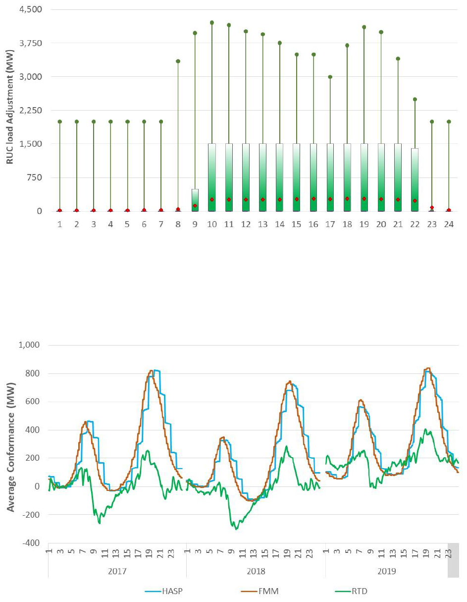
Figure 23 shows the monthly trends for load adjustments made to the RUC forecast, while Figure 24 shows

the same data organized in an hourly profile. During July 2018, when the system experienced load peaking

conditions and there were uncertainties about ramp and load forecast, the RUC adjustment maxed at

4,205 MW.

Figure 23: Monthly profile of RUC load adjustments

These additional requirements imposed by the load adjustments will be met with supply scheduled in

RUC. Some resources –internal generation and interties– will be incrementally scheduled above the IFM

schedules. In other cases, such RUC adjustments may lead to additional unit commitments that may be

binding for the trading day in RTM, i.e., they will be committed per RUC instruction, since there is no

sufficient time for re-optimization in the RTM. In such cases, the RUC adjustment will have a material

impact on the commitment of supply resources in RTM. The summer months have seen the majority of

the RUC adjustments and they typically apply in the ramp and peak hours of the day.

MQCRA/MA&F/GBA 27

Figure 24: Hourly RUC adjustments

In the real-time markets, the overall load requirements include the CAISO load forecast, exports, any load

conformance as well as system losses. Figure 25 illustrates the simple average of load conformance

applied to the real-time markets in an hourly profile and with a real-time interval granularity.

Figure 25: Hourly profiles of load conformance in the real-time markets

MQCRA/MA&F/GBA 28

These adjustments can effectively increase or decrease the overall demand requirements that the market

optimization uses to clear against supply. Operators may use load adjustments to true up the market to

the real-time system based on projected or observed system conditions.

Figure 26: Monthly distribution of load conformance used in the HASP market

Figure 26 through Figure 28 show the pattern of load conformance imbalance in the FMM and RTD

markets for 2018 and organized by month. Similar to previous discussion on prices, simple averages may

not show the more complex dynamics of t conformance. The box covers the 10

and 90

percentile while

the whisker covers between the minimum value and the 10

percentile, and the 90

percentile and the

maximum value of the samples. The line market within the box stands for the 50

percentile while the

red dot shows the simple average

. This trends show that the real-time markets have been frequently

clearing with an adjustment to the load forecast; these adjustment effectively imposed additional

requirements to meet with available supply.

The load conformance applied to the HASP and FMM markets align very well and follow a close profile

mimicking the load profile. In contrast, the load conformance applied to the RTD market divergence from

HASP and FMM and has a less defined hourly profile. The profile of the HASP and FMM conformance may

suggest the main driver is to position these markets to the real-time conditions while the RTD

conformance is to manage more the minute-to-minute imbalances in the real-time system. In each of the

markets, the spread of the load conformance is wide, ranging from -2,500MW to 3,000MW.

These figures show that HASP conformance applies predominantly in the upward direction. For instance,

it shows that from July 2018 through March 2019 more than 90 percent of the time the HASP conformance

The data sample used to determine the percentiles includes also the data points in which the load conformance

was zero MW, which effectively means there was no conformance applied to that interval.

MQCRA/MA&F/GBA 29

was an increase to the load forecast. Only in the transitional months, such as March and April, a higher

frequency of conformance was applied in the downward direction, which may be attributed to handle the

low-load conditions, high penetration of hydro and VER resources coming to full production. FMM

observes a similar pattern of conformance.

Figure 27: Monthly distribution of load conformance used in FMM

Figure 28: Monthly spreads of load conformance in the RTD market

MQCRA/MA&F/GBA 30

Figure 29: Hourly spreads of load conformance in the HASP market

Figure 30: Hourly spreads of load conformance in the FMM

MQCRA/MA&F/GBA 31

Figure 31: Hourly spreads of load conformance in the RTD market

MQCRA/MA&F/GBA 32

Load and Market Requirements

Changes to the load forecast itself can lead to misalignments between markets given the fact that

different markets use different look-ahead horizons. In cases of poor weather forecasts leading to

inaccurate load forecasting, the divergence between DAM and RTM could be significant. In the past, the

CAISO has analyzed extreme days, when missed temperatures forecast had a significant impact on the

load forecast accuracy. These inaccuracies, in turn, may lead operators to conservatively mitigate such

risks and uncertainties by securing more capacity through different operators’ actions, such as load

conformance or exceptional dispatches. Figure 32 through Figure 35 show the load forecast error for both

DAM and RTM, organized by month and by hourly profile. Not surprisingly, some of the most significant

errors, both under-forecasting and over-forecasting, have been observed when the system experienced

peaking conditions like September 2017 and July 2018.

In addition, these forecast errors appear to be more concentrated around the peak hours of the day,

which under extreme weather conditions happen to be the more uncertain periods. In some cases, the

forecasting error maybe over 3,000MW. As expected, the forecasting error is more significant in the DAM,

when there is an inherent time lag to actual conditions and rapid weather changes. For the RTM, with

more certainty of weather conditions and load evolution, the forecast errors will be inherently smaller.

Figure 32: Load forecast error in the day-ahead market

MQCRA/MA&F/GBA 33

Figure 33: Load forecast error in the real-time market

Figure 34: Hourly load forecast error in the day-ahead market

MQCRA/MA&F/GBA 34

Figure 35: Hourly load forecast error in the real-time market

As demand increases, the system may rely on higher priced bids to meet such levels of demand and, thus,

it is expected that price may rise accordingly and reflect the demand needs. While in the DAM the higher

price is often attributed to scarcity-driven conditions, in RTM, high prices are associated with more volatile

system conditions from interval to interval, temporal and ramp limitations.

Figure 36 shows a correlation between day-ahead prices and demand levels. For prices below $300/MWh,

a positive correlation is observed between prices and demand. At a higher range of prices, such correlation

becomes weaker, since there are cases in which for similar levels of demand prices can vary largely. This

is expected as demand levels is only one factors that defines the clearing prices. Higher and more volatile

gas prices is another factor. For similar levels of demand, if gas prices are different, it is expected that

electric prices will be different. For instance, the highest prices observed in the day-ahead market belong

to July 24 and 25, 2018. In addition to being the peak days of the year with relatively high loads, these

days also observed the highest gas prices, reaching up to $39/MMBTu. In contrast, there are many other

instances with load levels within same range but with much lower gas prices, which consequently result

in lower day-ahead prices. The correlation between electric prices, load levels and gas prices is shown in

Figure 36. The size of the bubble stands for the value of the gas prices; the higher the gas price the larger

the bubble depicted in the plot.

MQCRA/MA&F/GBA 35

Figure 36: Day-head prices correlated to demand level

The high energy prices observed in the market coincide with both higher load levels and high gas prices.

Hours with the highest load levels, like those of September 1, 2017, did not coincide with extreme gas

prices but still saw relative high electric prices. There are other instances with mild load levels but

relatively high electric prices due mainly to higher gas prices.

All of the CAISO markets optimally dispatch supply to meet the overall system load or bid-in. For the RUC,

HASP, FMM and RTD, the overall load that needs to be met with all available supply (internal generation

and imports) consists mainly of load forecast but also system losses and any load adjustments done by

operators. The difference between the load forecast and the actual market requirements can vary from

interval to interval, in the range of few thousands MW. This overall market requirement is effectively what

the market clears and relies on to set the prices. The divergence of these market requirements between

markets can naturally lead to price divergence because at a different market requirement to meet, the

market will clear at a different price level of the supply stack.

Figure 37 compares the overall market requirements across the different markets. For the IFM, there are

two variations of these requirements: one for physical supply, while a second version includes the

contribution of virtual bids (net between supply and demand). The former version is useful when

compared against the other markets that are based only on physical supply, while the latter provides a

reference of how much displacement (or convergence) the virtual bids introduced to the IFM. The

remainder of the markets also include any load forecast adjustments done by operators. These hourly

MQCRA/MA&F/GBA 36

trends are based on simple averages for each calendar year under analysis. The market requirements

diverge the most during the morning and evening peak hours. Both IFM and RUC tend to diverge more

from the real-time markets in the first hours of the day. One potential driver for this is explained in a

subsequent section below.

Figure 37: Total load across the various CAISO markets

Currently, VER resources have the flexibility to economically bid into the IFM. However, the CAISO has

observed that VER resources are consistently under-scheduling in the IFM as compared to the capacity

made available by these resources in the RTM. The ISO has since developed and implemented a true-up

process in RUC, where IFM bids for VER resources are increased to the forecasted generation values to

avoid over-committing generation in RUC. To the extent of the accuracy of the day-ahead VER forecast,

this functionality prevents over-generation conditions in the RTM arising from the under-scheduling of

VER generation in IFM that eventually will materialize in RTM.

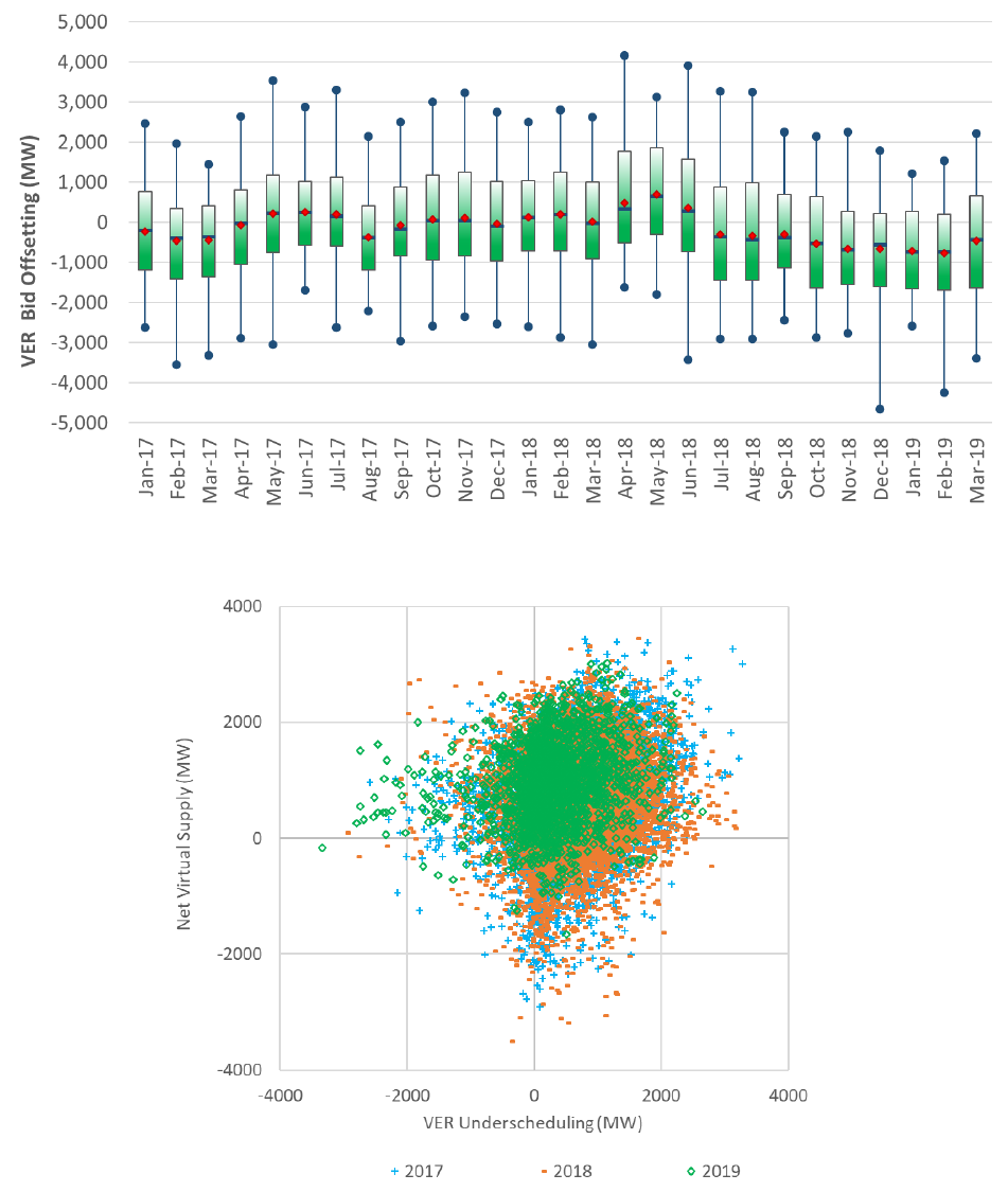
Figure 38 shows, on average, the difference between the VER supply considered in RUC in comparison to

the VER scheduled in IFM

. Overall, this is additional supply available in the RUC process to meet the day-

ahead load forecast, and is represented with blue bars.

This average applies to both solar and wind and may be skewed on the conservative side since it is over all hours

of the day, while solar may have no capacity for the first and last hours of the day. This metric will also be revised in

a subsequent version to take the maximum bid from IFM instead of the IFM schedule for VER. This current version

compares IFM schedules against VER day-ahead forecast; however, VER resources with economical bids in IFM may

be actually dispatched downward economically. The current metric does not differentiate between under-bidding

and dispatched downward economically in IFM.

MQCRA/MA&F/GBA 37

Figure 38: Average VER true-up up in the RUC process

Figure 39: Net load across the various CAISO markets

Currently, this true-up process is in place only for resources that bid into IFM. There may be cases in which

VER resources do not bid in IFM and this true-up process will not apply. Thus, there may be VER supply

still not considered in the RUC process that is projected to be available in the real-time market based on

MQCRA/MA&F/GBA 38

the VER day-ahead forecast; that additional capacity is identified with bars in red. Both types of capacity

followed the production pattern of renewables over the seasons.

Figure 39 provides an hourly profile on an annual basis for these two types of capacities associated with

VER under-scheduling. For all quarters of the year are considered for 2017 and 2018, but only the first

quarter is considered for 2019, due to the timing for doing the analysis.

Convergence bids

participate only in IFM and are liquidated in the real-time market at the FMM prices

because there are no physical resources to back them up. The main goal of virtual bids is to help converge

the day-ahead and real-time markets by identifying price difference to arbitrage, which may lead to more

efficient market outcomes. The RUC process does not consider virtual bids, but virtual bids can effectively

influence the commitment in the day-ahead market by displacing generation or creating additional

requirements for demand. One identified gap between the IFM and the real-time market is the VER under-

scheduling described above, so it is natural to expect that virtual bids can fill in that gap. Figure 40

provides the spreads of such convergence. This metric takes the difference of VER under-scheduling

between what was cleared in IFM and what cleared for VERs in the RTD market and compare s it against

the net virtual supply cleared in IFM

. A positive value is when the IFM under-schedule is greater than

the cleared net virtual supply. This hourly profile shows that there is a fairly large and symmetrical

distribution of how close virtual bids fill in for the gap of IFM VER under-schedule.

Figure 40: Hourly difference between IFM under-schedule and net virtual supply

The terms convergence bids or virtual bids are used interchangeably in this document.

The RTD dispatches are used in this metric because they are the ultimate supplied cleared by the market and that

materializes in a dispatch. However, other references can be taken for this metric; one could be the fifteen-minute

VER forecast or schedules under the premise that virtual bids are actually liquidated in FMM. The ISO may further

explore these variations in subsequent analysis.

MQCRA/MA&F/GBA 39

Similar spreads can be observed when trended overtime as shown in Figure 41. It is important to realize

that there may be other drives, as discussed in this analysis, that also play a role in market divergence

and for which virtual bids can be playing a role.

Figure 41: Hourly difference between IFM under-schedule and net virtual supply

Figure 42: Comparison between IFM under-schedule and net virtual supply

MQCRA/MA&F/GBA 40

Figure 42 shows the correlation between IFM under-schedule and net virtual supply; the correlation is

grouped by calendar year. A large volume of records are concentrated in a small range, and in general,

there seems to be a weak correlation between these two variables.

Figure 43 takes a step further and compares the net load across the various markets by subtracting the

contribution to meeting demand from VER resources –both wind and solar. The net load helps quantify

concurrently the variations not only from load but also from VER resources. This helps measure the overall

uncertainty that each market has to handle by using historical variations. The calculation of the IFM net

load relies on the overall cleared market requirements, the net virtual supply and cleared VER schedules.

For the RUC net load, the calculation uses the overall market requirements, that include any RUC

adjustment from operators, and the day-ahead VER forecast. For real-time, the net load uses the overall

market requirements, which includes load conformance, as well as the real-time VER forecasts (fifteen-

and five-minute accordingly). In contrast to the gross load, the divergence of net load across the markets

reduces for the morning and peak hours. It appears that the variation of VERs across markets offsets to

some extent the variations in the gross load among the markets.

Figure 43: Net load across the various CAISO markets

This metric, however, is a simple average that may hide the more granular variations, which sometimes

may be offsetting between positive and negative values. The relative differences between the day-ahead

market and the real-time markets also provide helpful information to understand the potential drivers for

price performance. This metric follows closely the concept to calculate the differences for net load

between markets to determine the uncertainty used for the flexible ramp requirements

. Figure 44

The use of box-whisker plots allows for an intuitive graphical representation of the distribution of differences.

Since these differences are based on multiple data points, namely, load forecast, VER forecast clear values,

MQCRA/MA&F/GBA 41

through Figure 51 show the net load differences between IFM, RUC, FMM and RTD, in both hourly and

monthly trends.

All these trends show that there is a significant uncertainty in meeting the net load across the ISO markets;

maximum values for these uncertainties can be as high as 9,000MW. This may typically happen when the

variations of the load forecast (accuracy) compounds with the variations of VER resources. Effectively this

means that positioning the supply needs from the day-ahead period in order to meet the real-time

conditions may represent quite a challenge. Currently, there is no explicit market mechanism to reconcile

such uncertainty from the day-ahead to the real-time market, and currently it is left up to the real-time

market and operators’ judgment in some degree to ensure the supply is properly position to meet the

actual system needs. For an illustration consider hour ending 19 in 2018, the range of variation from IFM

to FMM can be anywhere between -7,800 MW and +5,000MW; this represent an uncertainty range of

more than 12,000MW at the peak hour.

Figure 44: Hourly profile of net load differences between IFM and FMM

dispatches, market adjustments at the interval granularity, some intervals may have a data quality issue as many of

these data points are not subject to corrections after the fact. The data used for metrics throughout this report have

been clean up to the extent possible. When one data point is of no good quality, the whole data set for that interval

is dropped. For instance, if there is a missing value for an RTD dispatch, all data points such as forecast, IFM

schedules, VER forecast, RUC forecast, etc., are also ignored to avoid false differences. About four percent of the

overall data set has been omitted in this analysis due to potential data quality issues.

MQCRA/MA&F/GBA 42

Figure 45: Hourly profile of net load differences between IFM and RTD

Figure 46: Hourly profile of net load differences between RUC and FMM

MQCRA/MA&F/GBA 43

Figure 47: Hourly profile of net load differences between RUC and RTD

Figure 48: Monthly profile of net load differences between IFM and FMM

MQCRA/MA&F/GBA 44

Figure 49: Monthly profile of net load differences between IFM and RTD

Figure 50: Monthly profile of net load differences between RUC and FMM

MQCRA/MA&F/GBA 45

Figure 51: Monthly profile of net load differences between RUC and RTD

MQCRA/MA&F/GBA 46

Exceptional Dispatches

Operators can instruct specific resources to follow certain dispatch instructions to start up, shut down,

transition to a higher or lower configuration, operate at a specific MW dispatch, not exceed a specific MW

value and/or not fall below a specific MW value. Generally, EDs are issued during the real-time market;

i.e. post-day-ahead market, but there may be conditions in which EDs can be d prior to the day-ahead

market.

This type of operator action can insert out-of-merit generation into the supply stack that otherwise would

not have been available given the economics of the market. This in turn may distort the otherwise

economical market clearing price, potentially resulting in lower prices (when more capacity is

exceptionally dispatched) or higher prices (when EDs limit the available supply). Furthermore, EDs may

cause discrepancy between the capacity cleared in the DAM and the capacity used to clear the RTM, and

hence driving price divergence.

Out-of-the-market intertie dispatches is a variation of EDs in which operators may agree to buy/sell

additional energy with scheduling coordinators. When looking to address system –wide conditions the

reference typically are bids that did not clear in the HASP market and may be potentially available, and

when looking to address congestion specific interties may be more appropriate. These dispatches on

interties are at a given negotiated price. The negotiated price is paid only to the intertie resources that

were dispatched out of the market, and does not set the price for the rest of the market. The agreed upon

intertie energy is made available to the market as tagged (fixed) energy (as opposed to an economic bid

that can be cleared based on market prices) and is used in the overall power balance. Generally, such

manual dispatches on interties happen after the HASP market run. Depending how quickly the participants

submits the tag for the negotiated energy, the intertie energy may not be available for some of the

intervals of the hour. The out-of-market negotiated energy at the ties is a less frequent event than the

EDs issued for internal resources and are generally occur with constrained system conditions or projected

high levels of uncertainty. These will lead to a supply discrepancy between the HASP, and the FMM and

RTD markets, which in turn may influence the clearing prices, with higher prices in the HASP market and

lower prices in the FMM and RTD markets.

Over the years, the CAISO has developed different metrics and discussed to quantify the volume of manual

interventions in the CAISO markets. For example, the ISO closely tracks and reports EDs in different

forums, including the FERC monthly reports (Table 1 and Table 2), 120-days FERC report, monthly market

performance report, and Market Performance Forum Meetings. Anecdotally, the ISO has discussed

implications of EDs and other market interventions. In this analysis effort, the ISO is seeking to not only

more comprehensively quantify the extent of market interventions but most importantly to correlate,

identify, and to the extent possible, quantify their effect on price performance; namely, the impact that

the EDs creates on price performance.

Figure 52 shows the monthly volume of energy associated with all EDs, including intertie schedules, during

the 2018 calendar year, organized by reason. The largest volume of EDs occurred during the summer

months. Figure 53 shows the volume of energy issued with all exceptional dispatches averaged across

MQCRA/MA&F/GBA 47

hourly intervals during the 2018 calendar year. Exceptional dispatches are issued in higher volumes during

peak hours

Figure 52: Volume of Exceptional Dispatches in the CAISO market

Figure 53: 2018 Volume of exceptional dispatches in the CAISO market

Following discussion on the summer performance, the ISO worked on better classify prospectively the reasons for

exceptional dispatches because the load forecast uncertainties group was accounting for other types of uncertainties

such as fire risks.

MQCRA/MA&F/GBA 48

Figure 54 organizes the volume of exceptional dispatches in two groups, one for internal generation and

another for intertie resources. Generally, exceptional dispatches on interties is about 1 percent of the

overall volume in the reported period, even though in the months of August and September 2017, the

interties represented up to about 10 percent of the total volume of exceptional dispatches. These interties

can be for either imports or exports; exports are generally associated with emergency energy to other

balancing areas.

Figure 54: 2018 Volume of exceptional dispatches by type of resources

The IFM clears supply with bid-in demand based on the economics of the bids. The cleared IFM demand

may not align with the ISO load forecast for next trading date, thus, the RUC process is in place to ensure

sufficient capacity is procured to meet the forecasted load

. Resources committed in the RUC process, or

after the IFM, may result in additional capacity being available in the RTM than IFM. Consequently, this

may lead to lower RTM prices relative to those in IFM.

However, with the existing RUC provisions, RUC cannot de-commit resources from IFM; this may be of relevance

for periods of oversupply, and low or negative prices.

MQCRA/MA&F/GBA 49

Detailed Analysis of Price Performance

While overall trends aid pattern observation, analyzing specific market outcomes can help complement

and unravel dynamics in the price construct. For this type of analysis, the ISO took some of the instances

identified in previous sections with the largest price divergence between markets. Below is a sample of

deeper analysis undertaken to understand specific cases of price performance.

Price divergence in July 2018

As discussed in the analysis and trends in previous sections, July 2018 is a month in which the ISO observed

large and system-wide price divergence. This makes it an ideal month on which to perform more detailed

analysis to understand the underlying drivers of observed price performance. Figure 55 and Figure 56

show a more granular trend of prices for the month of July 2018, on a daily and hourly basis.

Figure 55: Daily system-weighted price across the CAISO markets

IFM prices were higher than the real-time prices on average for 29 days in July 2018, indicating a persistent

trend. When this pattern is organized by trading hour, the largest divergence is observed during the peak

hours. In particular, July 24 and 25 saw the largest price divergence between IFM and the real-time

markets as shown in the box-whisker plot in Figure 57. The divergence of average prices between the

various real-time markets, as illustrated through price spreads, are in general less frequent and are

characterized by a smaller range of spreads. Naturally, the real-time market may observe more volatile

prices that may lead to outliers in the spread, as shown in Figure 58 and Figure 59.

MQCRA/MA&F/GBA 50

Figure 56: Hourly system-weighted price across the CAISO markets. July 2018

Figure 57: Price spreads between IFM and HASP markets. July 2018

MQCRA/MA&F/GBA 51

Figure 58: Price spreads between HASP and FMM markets. July 2018

Figure 59: Price spreads between FMM and RTD markets. July 2018

MQCRA/MA&F/GBA 52

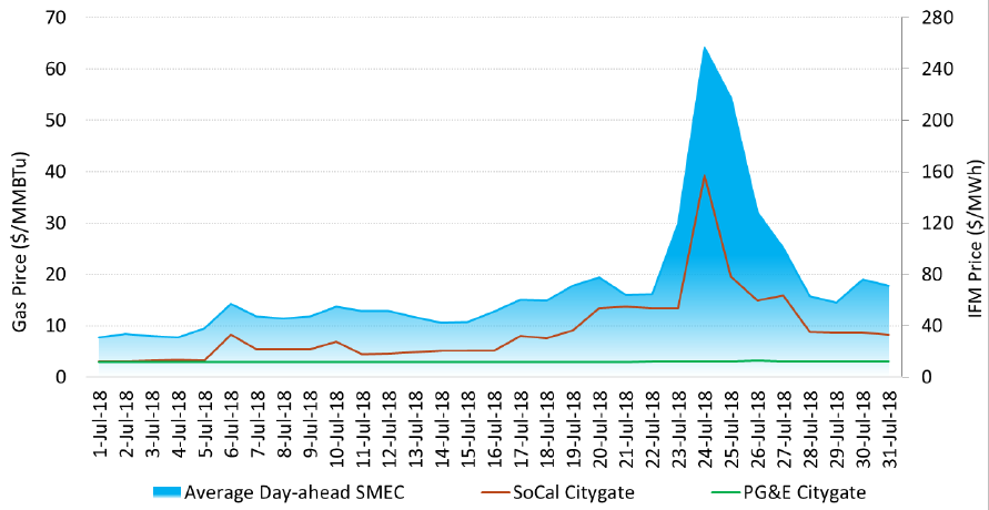
The month of July 2018 was operationally challenging; gas prices in Southern California were volatile and

particularly high on July 24 and 25, reaching about $39/MMBTu. Figure 60 shows a more granular trend

of the correlation between electric and gas prices. Given the meaningful contribution of gas resources to

the electric system and their tendency to be marginal, such high gas prices consequently led to high

electric prices. While the high gas prices can explain the high electric prices observed in IFM, they may not

fully justify a large price divergence between IFM and the real-time markets.

Figure 60: Electric and gas prices in the CAISO IFM

High temperatures that led to peak load conditions was a key factor during the month of July. CAISO

experienced the peak demand of the summer on Wednesday, July 25. This day was the third week day of

heat buildup experienced throughout the state of California. During this week, all regions experienced

above-normal maximum temperatures, minimum temperatures, and average temperatures throughout

the day exceeding these values by 2 to 12 degrees. This summer season was characterized by record-

breaking heat in coastal cities with San Diego reported its warmest August since records began in 1939

averaging 78.1 degrees Fahrenheit, 6.5 degrees above normal. In addition, Los Angeles reported its 3rd

warmest July since records began in 1877 at 78.8 degrees Fahrenheit, 5.5 degrees above normal. Inland

areas also saw records with Fresno setting a record all-time hottest calendar month at 88.2 degrees

Fahrenheit, 5.2 degrees above normal. One specific factor observed this summer is the record warm

minimum temperatures, which can have a big impact overall on the mean temperatures throughout July

and August, leading to potential higher loads in the electric system. With such challenging conditions, the

ISO system observed significant forecast errors in the day-ahead timeframe.

Figure 61 shows a comparison between the price spreads (HASP-IFM) against the maximum day-ahead

load forecast error. The largest errors, some in excess of 2500 MW, were observed on July 25 (the peak

MQCRA/MA&F/GBA 53

day of the year) and July 26

. Although the load forecast is not used directly in IFM, the challenging

conditions may affect the IFM because bids into this market may rely on forecasted conditions for the

trading date. If the ISO forecast observed such an error based on the temperature errors, other forecasts

used by SCs for bidding purposes may also suffer similar challenges. On these two days, the day-ahead

market was overscheduling the load. With such increased load requirements, the RUC market may have

committed excess resources to meet the lower actual load realized in the real-time markets. July 25 and

subsequent days had the largest over-forecasting error and coincide with the period with the largest price

divergence between day-ahead and real-time market.

Figure 61: Price spreads compared with day-ahead load forecast error in July 2018

July 25th was also the day with the largest price spreads, making it a good candidate to further explore

the conditions leading to such divergence. Figure 62 shows comparison across the various CAISO markets

of what each market cleared against supply. The market requirement determines that enough supply is

available to meet demand including any system losses and operator adjustments to the load forecast (i.e.

the RUC adjustment in RUC, and load conformances in HASP, FMM and RTD). For IFM, this is the total

demand cleared in the market, including losses. Accordingly, this measure compares the load

requirements across the markets on the same basis. There are two lines to represent IFM, one is for

physical demand only which can be a good reference against RUC requirements, and a second one that

includes the displacement introduced with net virtual demand. In this specific day, the net virtual was net

supply for all hours and effectively converged the IFM requirements closer towards the real-time

requirements. This brought IFM closer to the real-time conditions since IFM physical and RUC were

The load forecast errors have a sign convention to reflect overscheduling with a negative value.

MQCRA/MA&F/GBA 54

clearing above the actual conditions for that day. RUC used an over-forecast for this day and, given the

uncertainties, operators had an additional RUC adjustment of 2,000MW.

Figure 62: Demand needs across the CAISO markets on July 25, 2018.

Figure 63: Gross and net demand requirements in IFM for July 25, 2018.

This meant that the capacity schedule in IFM based on physical resources was already in excess to meet

actual system conditions, and naturally cleared higher in the bid supply stack at a correspondingly higher

price. RUC dispatched even more capacity above IFM. Then, with the extra capacity scheduled in RUC, and

MQCRA/MA&F/GBA 55

real-time conditions coming lower than forecast, the real-time market may effectively have plenty of

supply.

Figure 63 compares the IFM prices with the gross and net demand requirements. The net requirements

are estimated by taking the gross requirement and subtracting the VER awards in IFM. As discussed in

previous forums

, the highest prices observed in the day-ahead market typically occurs at the peak of the

net load, which is when the more stringent ramping needs are observed in the system as the solar

production diminishes with sunset. During these forums, the ISO also discussed what type of resources

can actually set prices above $200/MWh. Marginality that defines prices can be beyond standard heat

rates from conventional units. In addition to conventional fuel generation, imports, proxy demand

resources, batteries or convergence bids can become marginal and set prices.

In the specific case of July 25, convergence bids were setting the price during peak hours. The ISO

performed a counterfactual analysis in order to see convergence bids’ effect on prices. The ISO took the

original solution of the day-ahead market for July 25 and reran the market with and without consideration

of convergence bids. Figure 64 shows the comparison of prices between these two reruns.

Figure 64: Comparison of IFM solution when virtual bids are not considered

In this simulation, IFM prices increased up to $1,000/MWh in the net load peak hours when convergence

bids were not included in the market. In the solution with convergence bids included, convergence bids

were the marginal bids during peak hours. In the rerun simulation (i.e. in the absence of the convergence

bids), proxy-demand resources were marginal at about $1,000/MWh. The use of the highest-price bids in

For a reference on this discussion please refer to http://www.caiso.com/Documents/Presentation-

MarketPerformance-PlanningForum-Dec11_2018.pdf

MQCRA/MA&F/GBA 56

the market simply reflects the fact that, for this day, there was a tight supply condition in the day-ahead

market leading the market to clear in the upper-end of the supply stack

The over-forecasting of the load partly explains this outcome. Although the load forecast is not explicitly

used in the IFM market, bid-in demand most likely relied on over-forecasts. A secondary effect on the IFM

is the determination of the operating reserves. Generally, the full amount of operating reserves are

expected to be procured from IFM while any incremental procurement is done through the real-time

market. One of the components that may determine the level of operating reserves is the six percent of

the load forecast

. Thus, if the load is over-forecasted, the operating reserves may also be over-

forecasted. For July 25, the IFM was experiencing an over-forecast and the potential for over-forecasting

the requirements for operating reserves was under 200MW. The hourly profile of this over-forecast of

requirements is illustrated in Figure 65.

Figure 65: Comparison of IFM solution when virtual bids are not considered

This additional requirement for operating reserves will put upward pressure in the supply stack available

and naturally will have the market clearing higher in the bid stack.

To compare the supply available in both the IFM and RTM, consider hour ending 20 for a reference.

Figure 66 shows a comparison of supply bid stacks between IFM and HASP. The bids below -150$/MW

are self-scheduled, which prices are associated with penalty prices. It can been seen that the total bid-in

This aspect of the margin on supply was part of the discussion on system market power; material is available at

http://www.caiso.com/Documents/Presentation-SystemMarketPowerAnalysisJune7_2019.pdf

Effective January 1, 2018 as per new standard BAL-002 the operating reserves requirements also account for the

PDCI schedules as part of largest single contingency. So either this component or the 6% of load requirement will

set the level of operating reserves: when loads are not that high, the PDCI schedules will typically set the

requirements; when loads exceed certain level, the 6% of load will set the requirements. On July 25, 2018 with

loads exceeding 45, 000MW, the 6% requirements set the level of operating reserves.

MQCRA/MA&F/GBA 57

capacity (MW) of the two markets is very close. The bids are tracking closely in the range of $150/MWh

to $850/MWh. There is a shift of bids in the range between self schedules and $150/MWh. Figure 67

and Figure 68 show the differences of bid-in supply between the IFM and HASP markets. The net

between these two sets is relatively small.

Figure 66: Bid stack for IFM and HASP markets. July 25

Figure 67: Bid supply in IFM that is not in HASP

MQCRA/MA&F/GBA 58

Figure 68: Bid supply in HASP is not in IFM

For a more targeted comparison, each resource’s bid is compared between markets. Even though the

capacities of bids can be the same, the bids may be priced differently between markets. Therefore, the

price distributions of bids could contribute to price divergence between DAM and RTM.

Figure 69 and Figure 70 show the price distribution of bids in both IFM and HASP, organized by the type

of resource. The statistics in the figures take a bin range of $50/MWh. For example, bids priced anywhere

between $100/MWh and $150/MWh are counted in the bin of $100/MWh. If there are bids from both

markets in a given bin, one bar per market will be depicted. If there are bids only in one market, then only

one bar will show.

Two sets of resources have major shifts of the bid prices. The first set concentrates at a lower price range

(less than zero), which can be explained by the fact that economical bids in IFM come now as real-time

self-schedules. These resources are primarily wind, solar, geothermal, and biomass, hydro, pump storage

and import. However, if some resources were infra-marginal in IFM in the economical range to the point

of influencing the market clearing price, by the time they become self schedule in the real-time market

they no longer influence the clearing price in terms of price, but only in terms of the capacity they displace

in the bid stack.

MQCRA/MA&F/GBA 59

Figure 69: Bid price distribution

MQCRA/MA&F/GBA 60

Figure 70: Bid price distribution by resource price

MQCRA/MA&F/GBA 61

Price divergence on March 1, 2018

On March 1, 2018, in hour ending 19, the HASP price was about $48/MWh, the FMM interval 4 price

spiked to $1,000/MWh, and the RTD interval 12 price was about $36/MWh. These price differences were

driven by differences in load conformance across the real-time markets.

Four elements caused the FMM to clear an additional 1,300MW more than HASP: 1) load conformance

was 500MW higher in the HASP market in comparison to the conformance used in FMM; 2) the load

forecast came in 500MW higher in the FMM timeframe; 3) an increase of over 100MW in a particular

export; and 4) renewable resources came in about 200 MW lower in FMM than originally shown in the

HASP market. Clearing this higher load level naturally set the market in a higher range of the supply stack

where higher prices can be expected. Figure 71 shows the load conformance profile across the various

real-time markets for the period under analysis. The interval circled in yellow illustrates the large delta of

conformances. Then, when the RTD market ran, the price dropped to $36/MWh as a primary result of

having a load conformance of -350MW, which was a reduction of load of 1,450 MW with respect to FMM.

Figure 71: Load conformance across the real-time markets

The flexible ramp capacity that was procured for the system was in the range of 900 MW for the entire

EIM area footprint. About 620 MW out of that was procured within the PAC West area. However, this was

undeliverable to the ISO due to transfer (ETSR) limitations into the ISO creating a situation where flexible

ramp capacity is procured and then gets stranded due to transfer limitations. These types of situations

were addressed later in 2018 with a software enhancement that took into consideration the transfer

capability when awarding flexible ramp. The remaining of the flexible ramp capacity was procured within

ISO area, with about 50 MW not being deliverable due to gas limitations imposed in the market. The rest

MQCRA/MA&F/GBA 62

of flexible capacity (about 133 MW from conventional generation and about 96 from proxy demand

resources) was dispatched in FMM but was not sufficient to absorb the changes observed in FMM.

The export that increased by 100MW was not an actual intertie resource but rather a record introduced

in the real-time market reflecting the consideration of losses between the CAISO balancing area and an

adjacent area. This specific instance of in-kind losses is only in the FMM and RTD timeframe; neither the

HASP market nor the IFM consider this additional requirement, and may create a modest, but relatively

persistent, misalignment between the IFM and HASP versus the FMM and RTD markets.

Price divergence on September 5, 2017

On September 5, 2017, in hour ending 18, the IFM price was $74/MWh, the HASP price was $76/MWh,

RTD interval 7 price was $80/MWh, while the FMM price spiked to near $1,000/MWh.

Forecasting differences and outages drove these price divergences. On September 5, California system

and parts of the West were experiencing the end of a heat wave. The ISO load levels during this hour

where over 43,000MW. For HE18, the real-time forecast came in about 1,000MW higher than forecasted

in the day-ahead. There were also losses of over 700MW due to generation outages when going from day-

ahead to real-time. HASP had run with the forecasted loads, renewable levels, tie capacities, and resource

schedules that had been determined at the start of the run. However, by the time FMM ran for this hour,

there had been over 250 WM of tie cuts at SYLMAR due to a derating of a line and about 70MW of

additional exports to address losses with another balancing area. The load forecast increased 846 MW,

renewable forecast decreased 117 MW, and two resources were lagging or didn’t start, resulting in a loss

of over 450 MWs in comparison to HASP. Additionally, in the RTD market, the VER forecast increased by

430 MWs and the load conformance was 1,100 MW lower than it had been in FMM also leading to price

divergences. EIM transfers helped address this loss by contributing 500 MW but weren’t enough to cover

the lost supply and demand increases.

Price divergence in March 1, 2019

On March 1, 2019, in hour ending 14, FMM interval 4, the prices at the scheduling point for the NOB

intertie diverged across markets: IFM saw a price of about $151/MWh (with $113/MWh of marginal

congestion), HASP had a price of $999/MWh , FMM had a price -$9.85/MWh (with -$67/MWh of marginal

congestion) while RTD saw a price of -$20.5/MWh (-$113.78/MWh of marginal congestion). The daily

price trend for NOB intertie is shown in Figure 72.

MQCRA/MA&F/GBA 63

Figure 72: LMPs at the NOB scheduling point for March 1, 2019

The main concern in this case is the large divergence of the HASP market with respect to IFM, FMM and

RTD markets which can be attributed to weather conditions, gas market dynamics, and transfer issues.

An intense late-season polar cold blast led to large natural gas spot price increases on March 1, including

a record-setting spike in the Pacific Northwest

. The high natural gas prices drove high energy prices for

cities like Portland, OR and Seattle, WA. In the IFM, the NOB inter-tie had a zero MW limit in the export

direction and 1,622 MW in the import direction. The constraint was binding in the export direction based

on economical bids for both imports and exports at a shadow price of $151.68. For the HASP, the IFM

awards are self-scheduled, implying a net zero MW flow. Additionally, there were self-schedule export

bids for volumes greater than the economical bids in the import direction. Because the self-schedule could

not be fully offset with the economical import bids, the export bids were curtailed. This leads to

$1,000/MWh price based on a penalty price for constraint relaxation. In the HASP market, the NOB intertie

was binding at the shadow price of about $952/MWh which was set by the export bid. In this case, the

HASP market resolves the overscheduling and achieves feasibility for the tie limit. Once the FMM and RTD

markets ran and the cleared schedules from HASP were shown as tagged values, no congestion

management was needed on NOB and the tie was no longer binding. Additionally, there was congestion

from other constraints, such as the 30060_MIDWAY_500_24156 and VINCENT _500_BR_2 _3 lines,

contributing to the marginal congestion component at NOB scheduling point.

Source: https://www.naturalgasintel.com/articles/117595-sumas-hits-200-mark-as-natural-gas-spot-markets-

soar-on-cold-blast-futures-tepid

MQCRA/MA&F/GBA 64

Price divergence in June 19, 2017

On June 19, 2017, in hour ending 19, FMM interval 2, prices were about $116/MWh, $498/MWh,

$1,984/MWh and $49/MWh in IFM, HASP, FMM and RTD, respectively.

Two main items explain the large divergence of the FMM prices. First, an additional requirement of 700

MW through load conformance compounded with an increase in load forecast with respect to the HASP

market while solar ramping down contributed to a tighter supply condition. Second, a solution for this

particular market could not be improved further within the time the market had to run producing what

seemed to be a suboptimal solution. This same market was rerun with more recent software version and

the solution looks more optimal and prices reduced by about half of the original prices.

Price divergence in March 3, 2019

On March 3, 2019, in hour ending 17, FMM interval 1, the price at the Malin scheduling point (MALIN_ISL)

diverged significantly in the HASP market. In this interval, prices were $52/MWh, $1000/MWh, $10/MWh,

and $14/MWh in the IFM, HASP, FMM and RTD markets, respectively.

When the DAM ran, two outages on MALIN_ISL limited the export capacity. These were the OMS 6081202-

Roung Mountain Table mountain line outage and OMS 6081202-VACA Tesla series compensator outage,

the latter of which limited the export direction on the tie to 1465 MW. When the DAM ran, these outages

were expected to be completed by 9AM (or hour ending 10) and then the capacity would go up to 2450

MW. However, the outages did not return by that scheduled time. So in HASP for hour ending 17, the

export operating transfer capacity (OTC) limit was 1463 MWs. In the ISO markets, there is functionality to

protect for Existing Transmission Contracts (ETCs) and Transmission Operating Reservations (TORs)

contracts. These contracts are most often 75-minute contracts meaning that they can be used up till 75

minute before the hour. If the contracts are not used prior to that time, the capacity must be reserved.

Effectively that capacity is not available to the markets to be optimized. This results in an Available

Transfer Capacity calculation for un-used ETCs or TORs prior to the contract expiration. T-75 contracts are

still considered in the HASP. Because of this, the ATC in the HASP run was much less than OTC capacity to

reserve the capacity un-used ETCs and TORs. Because of this ATC being much lower than the DA ATC, DA

export schedules had to be cut in the HASP market resulting in the high price in HASP. Due to the cuts in

HASP making flows feasible but also with the release of the ETC and TOR contracts capacity into the FMM,

this constraint was no longer binding and FMM prices were within reasonable economical range.

MQCRA/MA&F/GBA 65

Scheduling of VER resources in IFM

Currently, VER resources can participate in IFM with same flexibility as conventional resources. They may

use a self-schedule or an economical bid. When it comes to the real-time market, their bids are capped

by the CAISO forecast even if they have economical bids. RUC uses similar logic. However, in IFM VER

resources are not limited in their bids by the CAISO forecast since this is a financial market. Historically,

because VER resources have under-scheduled in IFM, the ISO developed a logic to true up VER bids up to

the forecast level in the RUC process so that RUC can better determine the supply needs for the real-time

market. If this true up is not implemented, RUC will fail to consider additional VER capacity that is

forecasted to be available in the real-time and may over-schedule resources in RUC.

The ISO expects that under-scheduling of VER resources in IFM can be offset with virtual bids. Through

this analysis effort, the ISO found that some VER resources are actually over-scheduling in IFM. This is

more visible for solar resources bidding up to their maximum capacity in hours with no sunlight, such as

in the first six hours of the day and the last four hours of the day, clear times when conventional solar

resources cannot produce.

Figure 73: Solar production profile for March 31, 2019

For instance, consider the VER bidding and dispatches for March 31, 2019 represented in Figure 73 and

Figure 74. The solar profile has a flat line of about 2300 MW for the first six hours of the day and the last

four hours of the day. This is driven by about three dozen resources bidding up to their maximum capacity.

Since these resources will not be able to produce at this level in the real-time market, this volume will be

liquidated in RTM at real-time prices. Effectively, these VER bids are acting like virtual bids without being

MQCRA/MA&F/GBA 66

virtual bids and without the settlements implications for virtual bids. For reporting purposes, this bidding

also blurs the tracking of VER scheduling as it does not reflect forecasting or actual production conditions.

Figure 74: Wind production profile for March 31, 2019

RUC adjustment for day-ahead market of July 8, 2018.

As described in previous sections, based on projected conditions operators may adjust the RUC forecast

to ensure the proper capacity is positioned for RTM. During the month of July 2018, RUC adjustment were

significant. However, these adjustments to the load forecast do not necessary have a straightforward

impact on what resources will be committed for the real-time market. If 1,000 MW of additional

adjustment is imposed on RUC, it does not mean the market will commit an additional 1,000 MW of

generation relative to the IFM solution. For a more detailed analysis, July 8, 2018 was chosen because this

was the day in which the largest adjustment to the RUC forecast was applied (in the order of 4,250 MW

in hour ending 8). These adjustments effectively increased the overall RUC requirement that the market

takes as the reference to clear against supply. Figure 75 shows the profile of the RUC adjustment and the

RUC requirement with and without the adjustments, and compares it with the reference of what IFM

cleared. The original case that included the RUC adjustment was modified to take out such an adjustment

and then this modified DAM was rerun in order to compare the original solution with the adjustment

versus the solution obtained after removing the RUC adjustment. This comparison can help quantify the

impact of the RUC adjustment on the original market solution.

Figure 75: Demand requirements in the day-ahead market of July 8, 2018

MQCRA/MA&F/GBA 67

The additional requirement imposed by the adjustment increases the need for additional capacity to be

cleared in RUC. Figure 76 shows the additional capacity cleared by having the additional RUC requirement.

This capacity is organized by the type of dispatch and the type of resource procuring for the additional

requirement. First, in the early hours of the day when the additional requirements reached 4,250 MW,

the market run was actually infeasible to meet such capacity. The bars in brown show the amount of

capacity from the RUC adjustment that could not be procured in RUC, which reached about -1,400 MW.

Figure 76: Incremental RUC capacity due to operator adjustment

MQCRA/MA&F/GBA 68

This capacity was not procured because the power balance constraint was relaxed instead. From the

capacity that was actually procured to meet the RUC adjustment, over 80 percent was achieved by

incrementally dispatching resources already committed. Such capacity has no direct impact on the pool

of resources that are made available to RTM since it does not involve additional commitment instructions.

The majority of such incremental capacity was procured by dispatching up MSG units and other non-MSG

thermal resources, as well as some imports and proxy demand resources.

For the resources that were committed due to the extra RUC requirement, only two resources, amounting

to less than 200 MW, had a RUC binding commitment. This status refers to the condition in which the

resource commitment is defined in the DAM since the RTM cannot re-optimize its commitment. Thus the

start-up instruction from RUC is binding and will lead to the resource to be online for the real-time market.

Finally, for resources dispatched incrementally due to the additional RUC adjustment, a certain level of

that dispatch will be naturally covered by resource adequacy capacity and will have no associated costs in

the RUC market. The capacity above the RA level is identified as RUC awards and will be have associated

payments based on RUC prices. Figure 77 compares the RUC awards between the rerun market with no

adjustments and the original RUC awards due to the additional RUC adjustments; relatively speaking these

were modest RUC awards given the level of the adjustments. For instance, in hour ending 8 when the net

requirements adjustments were over 2,500MW, the RUC awards were less than 200MW.

Figure 77: Comparison of RUC awards for July 8, 2018

MQCRA/MA&F/GBA 69

Marginal Units

As part of the analysis of price performance, a typical concern is about marginality, i.e., what resources

are setting the price. In a given market interval, it is common to have more than one resource being

marginal due to all the constraints that may be binding in the market and also by the way bids are

constructed in step-wise format in the CAISO markets. Generally, resources will be cleared at the breaking

point between two segments and thus the standard concept of marginality where the bid equals the

clearing price may not capture all conditions of marginality. All type of resources in the CAISO markets

can set the prices. In particular, in the IFM, both supply and demand will be marginal, since demand can

participate with bids. In the RTMs, only supply will define marginal resources, since demand is inelastic

and defined by the load forecast. In IFM and HASP, however, exports which are equivalent to demand

may set the prices as well. Figure 78 and Figure 79 below shows the frequency of marginal resources

organized by the type of resources for day-ahead and real-time markets. This is presented in an hourly

profile for each quarter from January 2017 through March 2019. Each plot has both sides of the power

balance, showing the type of resources being marginal in the supply and also on the demand sides.

Figure 78: Marginal resources in the day-ahead market by type of technology

MQCRA/MA&F/GBA 70

MQCRA/MA&F/GBA 71

Figure 79: Marginal resources in the real-time market by type of technology

MQCRA/MA&F/GBA 72

MQCRA/MA&F/GBA 73

Proposed Plan for Analysis

This section summarizes the proposed plan for this effort. First, the initial scope of the analysis effort has

been identified and will be further revised based on feedback from stakeholders and the Market

Surveillance Committee. The second sub-section proposes deliverable phases and proposed schedules.

Scope of analysis

The following items have been identified as the initial scope of this effort:

1. Metrics to determine price performance – As previously stated, given the design of the CAISO

markets, price convergence across the different markets is a good indicator of a robust and

optimal market. There is a need to define metrics and meaningful ways to measure and identify

price convergence issues.

2. Operator interventions on the supply side. Over the years, the CAISO has developed different

metrics and discussed to quantify the volume of manual interventions in the CAISO markets. For

example, EDs are closely tracked and reported in different forums including the FERC monthly

reports (Table 1 and Table 2), 120-days FERC report, monthly market performance report, and

Market Performance Forum Meetings. Anecdotally, the ISO has discussed implications of EDs and

other market interventions. In this analysis effort, the ISO is seeking to not only more

comprehensively quantify the extent of market interventions but most importantly to correlate,

identify, and to the extent possible, quantify their effect on price performance; namely, the

impact on price divergence created by these market interventions, including

a. Exceptional dispatches of internal resources.

b. Manual dispatches of interties resources; this will include the various items raised by the

market surveillance committee about price formation concerns on interties.

c. Blocking of instructions.

3. Divergence of load requirements. All of the CAISO markets optimally dispatch supply to meet the

load forecast or bid-in load plus any operator adjustments. The CAISO will analyze

a. the market requirements for which the market cleared against in the various markets to

determine the effect of load requirement differences on price divergence. This will be

closely related to the analysis done on the divergence of supply capacity.

b. the effect of RUC net short adjustments in the RUC process and load conformance

imbalance in real-time markets.

c. the effect of load accuracy at different market timeframes. System load itself can change

among markets with no market intervention and such changes can create uncertainty on

system conditions, which in turn may lead operators to take actions to mitigate risks.

4. Divergence of supply capacity. The CAISO will analyze the divergence of supply capacity made

available across the markets either through the economics of the market or manual interventions

MQCRA/MA&F/GBA 74

to analyze its impact on price convergence and the potential incentives or arbitrage opportunities

that may be created across markets. This will include -

a. VER deviations across markets

b. Conventional resource deviations

c. The continuation of analysis on price formation previously discussed in the Intertie

Deviation Initiative for intertie resources, including the incentives and opportunities

created by divergence among these markets.

5. Dynamics of markets. The CAISO will also analyze -

a. the marginality of the markets; i.e., identifying resources which set the market clearing

prices, and conditions when prices are not reflective of fuel based conditions.

b. the effect of having only real time market consider EIM transfers into the CAISO system

and the resulting contribution to price divergence as compared to the day-ahead market.

c. the impact of convergence bids, and bidding more generally, in the different CAISO’s

markets, and the potential effect on price performance.

d. impacts of flex alerts, demand response into the market clearing of the real-time markets.

Stages of analysis

The analysis effort will be approached with two deliverables. In the first deliverable, the analysis effort

will be focused on measuring the various factors that may play a role in price formation. This will consist

of an initial report with a series of metrics, indices and trends of the multiple factors described in previous

sections of this report. In the second phase, the analysis objective will be to determine to the extent

possible, the correlations, causes, and effect of the areas identified in the first phase on price formation.

The analytical effort is itself an organic process that may be redirected based on findings throughout the

analysis. In very contained and insulated scenarios, the CAISO may be able to rerun some markets by

adjusting inputs or develop back of the envelope approximations to potentially quantify the effect of

certain factors. This analysis and associated discussions will inform potential solutions or enhancements

to improve the price performance.

MQCRA/MA&F/GBA 75

Proposed schedule

In order to provide opportunities for engagement and to shape the direction of this analysis, as well as to

discuss the analysis findings, the CAISO is planning to carry this analysis effort through a more formal

stakeholder engagement. The proposed timeline below highlights the main milestones.

Task

Schedule

Draft proposal for analysis

Monday April 3, 2019

Discussion at MSC meeting

Friday April 5, 2019

Stakeholder call

Wednesday April 10, 2019

Stakeholder comments

Wednesday April 17, 2019

Posting of first report

Monday June 17, 2019

Stakeholder call

Friday June 21, 2019

Stakeholder comments

Wednesday, July 3, 2019

Final report

Wednesday July 31, 2019

Stakeholder call

Wednesday August 7, 2019

MQCRA/MA&F/GBA 76

Appendix

This section provides additional metrics to complement the analysis and discussion presented in

previous sections.

Figure 80: Monthly comparison of average SMEC prices across the CAISO markets

Figure 81: 2017 Hourly comparison of average SMEC prices across the CAISO markets

MQCRA/MA&F/GBA 77

Figure 82: 2018 Hourly comparison of average SMEC prices across the CAISO markets

Figure 83: 2019 Hourly comparison of average SMEC prices across the CAISO markets

MQCRA/MA&F/GBA 78

Figure 84: Monthly system-weighted price spreads in IFM –Full price range

Figure 85: Monthly system-weighted price spreads in HASP –Full price range

MQCRA/MA&F/GBA 79

Figure 86: Monthly system-weighted price spreads in FMM –Full price range

Figure 87: Monthly system-weighted price spreads in RTD –Full price range

MQCRA/MA&F/GBA 80

Figure 88: Correlation between HASP and FMM load conformance

Figure 89: Correlation between FMM and RTD conformance

MQCRA/MA&F/GBA 81

Figure 90: Correlation between day-ahead prices and forecast error