The effect of upzoning on house prices and redevelopment premiums in Auckland, New Zealand

Article

Urban Studies

2021, Vol. 58(5) 959–976

Ó Urban Studies Journal Limited 2020

Article reuse guidelines:

sagepub.com/journals-permissions

DOI: 10.1177/0042098020940602

journals.sagepub.com/home/usj

The effect of upzoning on house

prices and redevelopment premiums

in Auckland, New Zealand

Ryan Greenaway-McGrevy

University of Auckland

Gail Pacheco

Auckland University of Technology

Kade Sorensen

University of Auckland

Abstract

We study the short-run effects of a large-scale upzoning on house prices and redevelopment pre-

miums in Auckland, New Zealand. Upzoning significantly increases the redevelopment premium

but the overall effect on house prices depends on the economic potential for site redevelopment,

with underdeveloped properties appreciating relative to intensively developed properties.

Notably, intensively developed properties decrease in value relative to similar dwellings that were

not upzoned, showing that the large-scale upzoning had an immediate depreciative effect on pre-

existing intensive housing. Our results show that the economic potential for site redevelopment

is fundamental to understanding the impact of changes in land use regulations on property values.

Keywords

house prices, land use regulations, redevelopment option, redevelopment premium, upzoning

Received April 2019; accepted June 2020

᪈㾱

ᡁԜ⹄ウҶᯠ㾯ޠྕݻޠབྷ㿴⁑㿴ࡂॷ㓗ሩᡯԧ઼䟽ᔪⓒԧⲴ⸝ᵏᖡ૽Ǆ㿴ࡂॷ㓗ᱮ㪇໎

࣐Ҷ޽ᔰਁⓒԧˈնሩᡯԧⲴᙫփᖡ૽ਆߣҾ൪ൠ޽ᔰਁⲴ㓿⍾▌࣋ˈ⴨ሩҾ儈ᇶᓖᡯӗˈ

վᇶᓖᡯӗॷ٬Ǆ٬ᗇ⌘᜿Ⲵᱟˈо㿴ࡂᵚॷ㓗Ⲵ㊫լտᆵ⴨∄ˈ儈ᇶᓖᡯӗⲴԧ٬л䱽ˈ

䘉㺘᰾བྷ㿴⁑㿴ࡂॷ㓗ሩݸࡽᆈ൘Ⲵ儈ᇶᓖտᆵӗ⭏Ҷⴤ᧕Ⲵ䍜٬᭸ᓄǄᡁԜⲴ⹄ウ㔃᷌

㺘᰾ˈ൪ൠ޽ᔰਁⲴ㓿⍾▌࣋ᱟ⨶䀓൏ൠ֯⭘ᶑֻਈॆሩᡯൠӗԧ٬ᖡ૽Ⲵส⹰Ǆ

ޣ䭞䇽

ᡯԧǃ൏ൠ֯⭘ᶑֻǃ䟽ᔪ䘹亩ǃ䟽ᔪⓒԧǃ㿴ࡂॷ㓗

Introduction

Upzoning is increasingly being advocated as a

solution to unaffordable housing (Freeman

and Schuetz, 2017; Glaeser and Gyourko,

2003). It refers to changes in regulatory land

use regulations (LURs) that enable more-

intensive site development (Gabbe, 2018).

Because LURs increase house prices by

restricting supply (Gyourko and Molloy,

2015), it is thought that a relaxation of these

regulations through upzoning can reduce

dwelling prices by enabling construction of

intensive housing (Freeman and Schuetz,

2017; Glaeser and Gyourko, 2003). Several

major cities in the USA have recently upzoned

large areas in response to rising housing costs,

including Minneapolis, Portland and Seattle

(National Public Radio, 2019).

However, our understanding of the

impact of upzoning on house prices is limited

by a lack of empirical research on the topic

(Freemark, 2019a; Schill, 2005).

Real option

theory suggests that upzoning might instead

increase house prices by enhancing the rede-

velopment premium embedded in property

values. The option to augment or tear down

and replace a residential structure can carry

a significant premium (Clapp and Salavei,

2010; Clapp et al., 2012a, 2012b) and upzon-

ing may increase the value of this redevelop-

ment premium by enhancing the extent of

permissible development on a parcel of land.

Understanding how these opposing apprecia-

tory and depreciatory effects of upzoning are

mediated by various factors, such as the

redevelopment potential of affected parcels,

the scale of the policy and the passage of

time, is critical to evaluating the efficacy of

upzoning to enhance housing affordability.

In this paper we examine the short-run

impact of upzoning on house prices using an

empirical method that distinguishes increases

in redevelopment premiums from other mar-

ket equilibrium effects of the policy, such as

increases in housing supply. Our study is

based on a policy intervention that upzoned

large areas within the metropolitan region of

Auckland, New Zealand (NZ). To analyse

the effects of this policy change, we embed a

difference-in-differences structure in a hedo-

nic pricing function, wherein an upzoning

quasi-treatment is interacted with a conven-

tional measure of site development: intensity.

Intensity is the ratio of the value of improve-

ments to the total property value and is often

used in empirical hedonic regressions to

measure redevelopment premiums because it

reflects the economic potential for site rede-

velopment (Clapp and Salavei, 2010; Clapp

et al., 2012a). Intuitively, the opportunity

cost in terms of foregone rent from tearing

down an apartment block (with a corre-

spondingly high intensity ratio) is much

greater than the opportunity cost of tearing

down a small house on a large land parcel

(with a low intensity ratio). The former

therefore has less economic potential for

redevelopment than the latter and corre-

spondingly carries a smaller redevelopment

premium. By conditioning on intensity, we

can isolate enhancements in redevelopment

premiums from other policy effects on

prices, such as decreases in prices due to

actual or anticipated construction. These

ideas are theoretically formalised in the third

section of this paper using the Clapp and

Salavei (2010) real option model.

We find that upzoning significantly

increases the hedonic estimate of the redeve-

lopment premium. However, the net effect

on house prices is decreasing in intensity,

meaning that underdeveloped properties

appreciate relative to intensively developed

properties. Further, upzoned properties that

Corresponding author:

Ryan Greenaway-McGrevy, University of Auckland, Economics, 12 Grafton Road, Auckland 1024, New Zealand.

Email: r.mcgrevy@auckland.ac.nz

960 Urban Studies 58(5)

exceeded a sufficiently high level of intensity

decreased in price relative to non-upzoned

properties, illustrating that the large-scale

upzoning had an immediate depreciative

effect on pre-existing forms of intensive

housing. The existing extent of site develop-

ment is therefore identified as a key attribute

mediating the appreciatory and depreciatory

impacts of upzoning. These results hold

under several robustness checks and placebo

tests.

This paper makes several contributions to

the literature. First, while a tremendous

amount of research has focused on the

static effect of cross-sectional variation in

LURs (see Gyourko and Molloy, 2015;

Pogodzinski and Sass, 1991; Quigley and

Raphael, 2005, for reviews), there has been

much less research on the effects of dynamic

changes in zoning restrictions, in part

because large-scale changes in regulations

are rare (Freeman and Schuetz, 2017).

break new ground on this understudied topic

by examining a policy intervention in which

most of the residential land in the metropoli-

tan urban area was upzoned. Second, by

identifying intensity as a key attribute med-

iating price effects, we reconcile the fact that

upzoning can decrease average dwelling

prices by enabling supply of more intensive

forms of housing, while increasing the value

of properties that are more-endowed with

land relative to those that are less-endowed,

as predicted by real option theory. In eco-

nomic terms, upzoning reduces the minimum

amount of land required to produce a dwell-

ing, and this increase in land productivity is

captured both by consumers, through lower

dwelling prices, and by landowners, through

larger factor payments to land. Because a

property is a bundle of land and dwelling,

the net price effect of upzoning depends on

the relative value of its land endowment.

Finally, our approach helps assess the cred-

ibility of market-led policies to improve

housing affordability. Housing construction

can be impeded by land assembly problems

(O’Flaherty, 1994) and other regulatory bar-

riers (Schill, 2005). Our hedonic model per-

mits us to price intensively developed (i.e.

high intensity) dwellings to uncover whether

prices on such properties decrease after the

policy is announced.

Our data set offers some unique advan-

tages that assist in identifying the effects of

upzoning. First, non-upzoned houses pro-

vide a quasi-control, thereby permitting a

difference-in-differences approach that miti-

gates some of the concerns related to the

endogeneity of regulations in the cross-

sectional setting (Gyourko and Molloy,

2015). Second, there is a unique identifier

for each property, which enables use of

repeat sales to control for time-invariant fac-

tors affecting house prices over the sample

period. Third, the dataset is sufficiently

detailed so that we can control for numerous

other potential confounding factors, such as

proximity to the central business district

(CBD). Finally, we can match the transacted

property to its residential planning zone, so

that we can pinpoint upzoning in space and

time, rather than estimating where and when

rezoning occurred.

The remainder of the paper is organised

as follows. The following section reviews the

extant literature on zoning, house prices,

and affordability. The third section contains

a detailed description of the institutional

background underlying our study. The next

section presents the theoretical foundation

for our empirical regressions. Empirics are

contained in the penultimate section and the

final section concludes.

Literature review

Numerous studies have analysed the rela-

tionship between zoning regulations and a

variety of outcomes, including house prices

and affordability, construction and rents

(surveys include Gyourko and Molloy, 2015;

Greenaway-McGrevy et al. 961

Pogodzinski and Sass, 1991; Quigley and

Raphael, 2005). The majority of studies find

that locations with more regulation have

higher house prices and less construction,

although planning endogeneity limits our

ability to infer causality from these correla-

tions (Gyourko and Molloy, 2015).

Nonetheless, empirical studies that account

for endogeneity frequently find that tighter

LURs cause increases in house prices

(Dalton and Zabel, 2011; Hilber and

Vermeulen, 2016; Ihlanfeldt, 2007; Jackson,

2016) and decreases in construction

(Chakraborty et al., 2010; Glaeser and

Ward, 2009; Jackson, 2016).

On the basis of this and other work,

many researchers argue that a relaxation of

LURs will improve affordability and acces-

sibility by enabling more housing construc-

tion (Freeman and Schuetz, 2017; Glaeser

and Gyourko, 2003; Manville et al., 2020).

Yet, many others remain sceptical of the

capacity for upzoning to deliver affordable

housing, arguing that benefits to lower-

income households are limited (Favilukis

et al., 2019; Rodriguez-Pose and Storper,

2020). Part of the problem is that our under-

standing of the manifold impact of upzoning

on prices is limited by an acute lack of

empirical research on the topic (Freeman

and Schuetz, 2017; Schill, 2005). Research

adopting a quasi-experimental approach to

examine price effects of zoning changes is

limited to Atkinson-Palombo (2010) and

Freemark (2019a). Notably, Freemark

(2019a) finds that multifamily buildings

appreciated relative to controls in Chicago

after transit-oriented upzoning.

In addition to upzoning, other policies

intended to reduce impediments to market-

led supply include relaxing urban growth

boundaries (Anacker, 2019); reducing unne-

cessary regulations and making the develop-

ment process more certain and transparent

(Freeman and Schuetz, 2017); and accelerat-

ing land-use and construction approvals

(Anacker, 2019). Other researchers instead

advocate for direct state intervention.

Wetzstein (2019) argues that non-market-

based housing supply, demand-side interven-

tions and urban land market interventions

are required to ensure housing affordability,

while Favilukis et al. (2019) show that direct

state-led interventions, such as vouchers and

accurately targeted inclusionary zoning,

more effectively enhance affordability in a

calibrated spatial equilibrium model.

Meanwhile Been et al. (2019) argue for a

broad policy package that includes both

state intervention and the removal of impedi-

ments to market-led construction. Freemark

(2019b) also advocates for a combination of

large-scale state-led intervention and regula-

tory reform, pointing out that housing unit

construction doubled in Paris after renewed

government support for affordable housing,

repurposing of public land, LUR reform and

the introduction of financial incentives for

private-sector construction.

Institutional background

Auckland is the largest city in NZ, with an

estimated population of approximately

1.7 million in 2017 (Auckland Council,

2017). The region covers 489,363 ha, of

which 50,550 ha constitute the core urban

area (Auckland Council, 2017). From

November 2010 the entire region fell under

the jurisdiction of the Auckland Council

(AC), formed after amalgamation of eight

different city and district councils. Auckland

has a population-weighted density of

approximately 4310 people per km

(source:

authors’ calculations based on 2013 census

data), and the population is evenly distribu-

ted outside the CBD (see Figure A1 in the

online Supplemental Material).

962 Urban Studies 58(5)

Auckland’s house prices roughly doubled

between 2009 and 2016 (see Supplemental

Figure A2), which resulted its housing being

ranked among the most unaffordable in the

world (Demographia, 2018). This increase

was predominantly unique to Auckland

within NZ. Prices have remained flat since

2016, coinciding with successive govern-

ments implementing policies to stem demand

and the central bank restricting credit

through tighter macroprudential policies.

Recent changes under the Auckland

Unitary Plan (AUP) make Auckland an

ideal case study to investigate the effects of

large-scale upzoning in a metropolitan area.

The AUP relaxed regulations to permit

increased density in large areas of the city

(Balderston and Fredrickson, 2014: 21). Key

milestones in development and implementa-

tion of the AUP are summarised below:



July 2010: The Local Government Act

2010 passed by the NZ government

requires AC to develop a consistent set

of urban planning rules.



15 March 2013: AC released the ‘draft’

AUP, followed by 11 weeks of public

consultation.



30 September 2013: AC released the

Proposed AUP (PAUP) and notified the

public that the PAUP was open for

submissions.



April 2014 to May 2016: An

Independent Hearings Panel (IHP) was

appointed by the NZ government and

subsequently held 249 days of hearings.



22 July 2016: the IHP set out recom-

mended changes to the PAUP. One of

the significant recommendations was

abolition of minimum lot sizes (except

for new subdivisions). AC considered

and voted on the IHP recommendations

over the next 20 working days.



19 August 2016: AC released the ‘deci-

sions’ version of the AUP. Several of the

IHP’s recommendations were voted

down but abolition of minimum lot sizes

was maintained.



8 November 2016: AC notified the pub-

lic through the media that the final AUP

version would become operational 15

November 2016.

All AUP versions (‘draft’, ‘proposed’, ‘deci-

sions’ and ‘final’) proposed new zoning regu-

lations that were easily viewed online. Any

interested member of the public could

observe the proposed regulations applying

to any given parcel in the city.

We focus on four residential zones intro-

duced under the AUP, listed in declining lev-

els of permissible site development: Terrace

Housing and Apartments; Mixed Housing

Urban; Mixed Housing Suburban; and Single

House. See Supplemental Table A1 for an

overview of the LURs by zone. These regula-

tions include site coverage ratios and height

restrictions, among others. For example,

between five and seven storeys and a maxi-

mum site coverage ratio of 50% is permitted

in Terrace Housing and Apartments, whereas

only two storeys and a coverage ratio of

35% is permitted in Single House. Together,

these four zones comprise over 90% of the

transactions in our sample.

AC estimated that the new zones

increased capacity for new dwellings by over

300%,

illustrating the large-scale nature of

the upzoning policy. Figure 1 depicts the

geographic distribution of the four zones

across the city. Mixed Housing Suburban is

the largest zone by area, covering 44.6% of

all residential land (source: authors’ calcula-

tions), while Mixed Housing Urban covers

22.5%. Single House is predominantly

located either very close to or at the CBD

outskirts, and covers 25.5% of residential

land. Terrace Housing and Apartments cov-

ers only 7.4% of residential land.

Our empirical design treats the AUP

announcement as a quasi-natural experiment

(where Single House acts as the control; see

Greenaway-McGrevy et al. 963

section ‘Econometric model’). We therefore

must select a time period ‘before’ and ‘after’

the treatment has occurred. Unfortunately, as

is clear from the timeline above, there is no

clean, singular announcement. We adopt a

conservative approach and take the years

between 2010 and 2012 (inclusive) as pre-

treatment (whic h pre-dates release of the

(first) draft AUP), and September 2016 to

December 2017 as post-treatment (immedi-

ately after the final ‘decisions’ AUP version is

released). We explore several other time peri-

ods in our robustness checks.

Theoretical framework

In this section we repurpose the Clapp and

Salavei (2010) real option model of housing

redevelopment to examine what happens to

property values when restrictions on devel-

opment are relaxed (as occurs under upzon-

ing). These theoretical predictions are

empirically tested in the following section.

Full details are provided in the Supplemental

Material.

The set-up is as follows. Each developed

property has a vector of characteristics q

that earn rents p and depreciate at rate d.

Future rents p (and characteristics q

) are

known with certainty. The property owner is

permitted to redevelop to the standard given

by q

. The cost of redevelopment is k qðÞ,

such that the construction costs are a func-

tion of q 2 R

, and where we assume that

k qðÞ. 0, so costs are positive. Then the

value of the property is

Figure 1. Residential zones in Auckland.

Notes: The dot close to the centre of the maps is the location of the ‘Skytower’ within the CBD. Solid black lines

demarcate coastline.

964 Urban Studies 58(5)

+ v

 q

ðÞk(q

)ðÞ

 k(q

)



r + d



ð1Þ

where v =

r + d

and r is the discount rate.

The redevelopment premium is the second

term. It disappears if q

= q

. We assume

v#(q

)>k(q

We consider what happens to V

when

the policymaker increases an element of q

that represents an overall measure of devel-

opment intensity (call it q

iðÞ

). We can there-

fore think of upzoning as an exogenous

increase in q

iðÞ

. By taking the partial deriva-

tive of V

with respect to q

iðÞ

(refer to the

Supplemental Material for details), we obtain

two key results to be empirically tested:

(1) An increase in q

iðÞ

through upzoning

increases the property value, all else

equal.

(2) The increase in property value is

decreasing in q

iðÞ

, meaning that a prop-

erty with a lower initial level of site

development will experience a larger

increase in price from upzoning, all else

equal.

Although the model abstracts from mar-

ket equilibrium effects of upzoning, such as

the impact of increased housing supply on

house prices, it can straightforwardly accom-

modate common changes in house prices

brought about by shifts in supply and

demand. If housing in upzoned and non-

upzoned areas become imperfect substitutes

after upzoning, this reasoning yields a third

prediction:

(3) Anticipated dwelling construction in

upzoned areas decrease property prices

in upzoned areas relative to non-

upzoned areas.

Thus, the appreciatory effects of upzoning

via the redevelopment channel (1) are poten-

tially offset or altogether dominated by the

depreciatory effects of increased construc-

tion (3). The relative magnitude of these

opposing effects is mediated by the extent of

site development, q

iðÞ

, as stipulated under

(2). For example, properties that are already

developed to the extent permitted after

upzoning might depreciate relative to simi-

larly developed properties that were not

upzoned, since these properties have no

redevelopment potential.

Note that effects (1) and (3) become evi-

dent by comparing outcomes in upzoned

areas relative to non-upzoned areas. Our

conceptual framework does not, therefore,

identify average changes in redevelopment

premiums and house prices across the city. It

does, however, permit us to uncover evi-

dence of these city-wide effects because it

suggests that upzoning manifests as a dis-

tinct and identifiable pattern in house price

changes between upzoned and non-upzoned

areas provided we condition on site develop-

ment. Specifically, (3) should manifest as

upzoned, pre-existing high intensity dwell-

ings appreciating relative to non-upzoned,

pre-existing high intensity dwellings.

Meanwhile, (1) manifests as underdeveloped,

upzoned properties appreciating relative to

underdeveloped, non-upzoned properties.

Finally, note that (3) can be consistent

with no overall increase in the city’s dwelling

stock if upzoning only reallocates antici-

pated future construction from non-upzoned

to upzoned areas. It is therefore critical to

carefully check for evidence of this potential

demand shift on house prices and, if neces-

sary, control for it, before concluding that

the policy generated an overall increase in

Greenaway-McGrevy et al. 965

anticipated dwellings. We explore this possi-

bility in our spillover robustness checks (sec-

tion ‘Treatment spillovers’).

Empirics

Data

Our primary dataset consists of all residen-

tial property sales in Auckland between 2010

and 2017 (inclusive). The dataset contains

various information on the transacted prop-

erties, including: the sales price (excluding

chattels); date of sale; assessed value of land

and improvements; land area (in hectares),

where applicable; floor area and site foot-

print (in square metres); whether the land

title is freehold or leasehold; dwelling type

(house, unit or apartment); number of bed-

rooms and bathrooms; decade of construc-

tion; latitude and longitude of the property;

and Area Unit (AU) in which the property is

located.

Each house has a unique identifier,

so we can track sales of individual properties

over time. We clean the data to remove

transactions that appear to have had infor-

mation incorrectly coded or omitted, that

appear to be non-market transactions or

that are not relevant to our study (see the

Supplemental Material for details).

We also identify properties with joint

ownership of the land underlying the build-

ing, such as apartments and cross-leases.

In our preferred specification we limit the

sample to titles with exclusive land owner-

ship, since redevelopment of these sites is

not affected by title assembly problems

(O’Flaherty, 1994). However, a robustness

check reveals that this has no impact on our

results (see section ‘Including properties with

joint land ownership’).

The intensity ratio plays a significant role

in our empirics. It is constructed as:

intensity =

= 1 

ð2Þ

where AV is total assessed value, LV is

assessed land value and IV is the improved

value (or capital value) of the property. IV

=AV2 LV holds as an identity. Assessed

values are based on local government valua-

tions for levying property taxes. The redeve-

lopment premium is decreasing in intensity,

meaning that negative coefficients on inten-

sity in hedonic regressions indicate a positive

premium. By construction the ratio lies

between zero and one, but the ratio does not

exceed 0.8 in our sample.

We use longitude and latitude to identify

the planning zone in which the property is

located, retaining transactions in the four

main residential zones introduced in the

third section: Terrace Housing and

Apartments (which we refer to as ‘Zone 4’);

Mixed Housing Urban (‘Zone 3’); Mixed

Housing Suburban (‘Zone 2’); and Single

House (‘Zone 1’).

Additional variables are generated and

employed as controls. We identify houses

with two or more storeys (by comparing

floor area to site footprint), we derive the

approximate building age (difference

between the date of sale and decade in which

the building was constructed),

and longi-

tude and latitude are used to calculate dis-

tance to the CBD.

To control for

neighbourhood income, we use the median

household income for the AU in which the

property is located.

Econometric model

Suppose that the policy is announced in time

period t

. Our regression is

i, t

 p

i, t

1

ðÞ= b

s = 2

zone

s, i

+ d

intensity

s = 2

zone

s, i

intensity

+ g

+ e

ð3Þ

966 Urban Studies 58(5)

where:



i=1,.,n indexes the transactions

(houses) in the sample.



i, t

1

is log sales price (excluding chat-

tels) of house i in period t

1

(i.e.

before the announcement); p

i, t

is log

sales price (excl. chattels) of house i in

period t

1

. A property is there-

fore included in our sample if it was sold

in period t

1

and in period t

. In our

baseline empirical specification, we use

the years 2010 through 2012 (inclusive)

for t

1

and September 2016 to December

2017 for t

, which leaves 2340 observa-

tions. If a house was sold more than

once within t

1

or t

, we use the first

transaction in the period.



denotes the years between the sale of

house i in period t

1

and period t

,so

that the dependent variable is an annual-

ised rate of inflation. The average num-

ber of years between transactions is 5.64.



fzone

s, i

s = 2

are upzoning dummies for

Zone 2, Zone 3 and Zone 4, respectively.

Thus m=4. The reference group is

Zone 1 (Single House).



intensity

is intensity (see eq. (2)) in

period t

1



is a vector of controls including prop-

erty attributes and neighbourhood infor-

mation: (log) land area; (log) floor area;

a dummy variable indicating two or

more storeys; number of bedrooms;

number of bathrooms; approximate

building age; (log) distance to CBD;

and (log) median household income for

the AU. We report regression results

with and without these controls.

Eq. (3) is the first difference of a conven-

tional difference-in-differences regression

where the treatment i s interacted with

intensity. In the Supplemental Material we

demonstrate this equivalence step-by-step.

Table 1 documents sample descriptive

statistics for the variables in the model.

Supplemental Table A2 contains these

descriptives stratified by residential zone,

showing that sales in zones that permit more

intensive development tend to be closer to

downtown and in suburbs with lower

incomes. Average intensity is similar across

all four zones.

Approximately one-quarter of the trans-

actions (25.5% = 597/2340) fall into the

Single House zone, which acts as our quasi-

control. 51.2% (= 1199/2340) are in Mixed

Table 1. Summary statistics.

Mean Median Std dev. Skew 1st perc 5th perc 95th perc 99th perc

Price appreciation 0.12 0.12 0.03 20.80 0.04 0.07 0.18 0.21

Intensity 0.43 0.44 0.13 20.25 0.10 0.21 0.63 0.70

Land area (ha) 0.07 0.07 0.03 4.85 0.02 0.03 0.11 0.18

Floor area (m

) 154.61 140.00 62.34 1.02 70.00 80.00 274.50 340.60

Bedrooms 3.48 3.00 0.74 0.40 2.00 3.00 5.00 5.00

Bathrooms 1.65 2.00 0.74 1.04 1.00 1.00 3.00 4.00

Building age (yr) 38.72 40.00 26.40 0.64 1.00 2.00 92.00 102.00

Dist. to CBD (km) 17.89 14.37 11.43 1.25 2.24 4.47 41.91 51.27

AU income

(NZ$ 000)

64.60 61.60 15.52 0.01 36.90 42.00 95.50 100.00

Notes: Price appreciation is the average annual change in log prices and is based on repeat sale residential transactions

between the pre-treatment sample (January 2010 to December 2012) and the post-treatment sample (September 2016

to December 2017). AU income is median household income (NZ$) in the Area Unit (suburb) of the transaction and is

obtained from the 2006 census. ‘Skew’ denotes skewness, while ‘perc’ denotes percentile.

Greenaway-McGrevy et al. 967

Housing Suburban and 18.3% (= 428/2340)

fall into Mixed Housing Urban. Only 5% (=

116/2340) of the transactions fall into the

Terrace Housing and Apartments zone, which

permits the most site development.

Several features of eq. (3) are worth

remarking on.

(1) The coefficients d

s = 2

capture the

effect of upzoning on the redevelop-

ment premium. Recall that the coeffi-

cient on the intensity ratio from

hedonic regressions is used to estimate

the redevelopment premium. The coef-

ficient d

therefore captures the change

in the redevelopment premium for the

reference group (Zone 1), which was

not subject to upzoning. In turn, coeffi-

cient d

captures the change in the

redevelopment premium for houses

located in Zone 4 relative to the change

in the redevelopment premium for

houses in Zone 1. A priori we expect

this coefficient to be negative since the

redevelopment premium is decreasing

in intensity and upzoning should

increase the redevelopment premium.

Similar statements can be made about

and d

for Zones 2 and 3.

(2) Because the dependent variable is the

change in individual house prices, the

empirical model controls for time-

invariant confounding factors affecting

house prices over the sample period. In

this regard, our approach is like that

advocated by Dalton and Zabel (2011)

and Gyourko and Molloy (2015: 1303–

1304), who suggest panel data can be

used to address the endogeneity of reg-

ulations. Note that our difference-in-

differences model is not based on a

repeated cross section (c.f. Freemark,

2019a), but a panel.

(3) The vector X

includes property attri-

butes and geographic characteristics to

control for any remaining confounding

factors that vary over the sample

period. For example, an increase in

transport congestion may have inflated

the premium for houses closer to

downtown, hence we control for dis-

tance to the CBD. Because the empiri-

cal model is a time-differenced hedonic

regression, the parameters associated

with X

can be interpreted as changes

in the hedonic coefficients on the attri-

butes between t

1

and t

Regression results

Column (A) in Table 2 reports regression

results. It includes results for when all con-

trols are omitted and when controls related

to the geographic characteristics (household

income and distance to downtown) are

omitted. See columns (B) and (C).

The coefficients on the three upzoning

dummy variables interacted with intensity

are negative and statistically significant.

This is strong evidence of upzoning increas-

ing the redevelopment premium (see Remark

(1) in the preceding section). Furthermore,

note that the magnitudes of these coefficients

correspond to the ordinal ranking of permis-

sible site development under each zone.

The coefficients on the upzoning dummy

variables (not interacted) are positive and

statistically significant, indicating that an

upzoned property with intensity of zero (i.e.

equivalent to an empty lot) appreciated rela-

tive to non-upzoned properties. The magni-

tudes of the estimated coefficients again

correspond to the ordinal ranking of permis-

sible development under each zone.

Interestingly, the coefficient on intensity

(not interacted) is statistically indistinguish-

able from zero. This suggests that there was

no change in the redevelopment premium

for the quasi-control group after the

announcement.

Next, to illustrate how the effect of

upzoning on overall house prices depends

968 Urban Studies 58(5)

on existing site development, we use the

estimated regression model to construct pre-

dicted changes in house prices conditional

on both the residential zone and the inten-

sity ratio. For each of the four zones,

Figure 2 plots the expected annualised price

appreciation conditional on intensity. For

this exercise we set the control variables in

to their sample means to construct pre-

dicted values.

First, we consider Zone 4, which permits

the most site development. Holding all else

equal, the model implies that houses located

in this zone appreciated by between 14.7%

(intensity = 0) and 9.3% per year (intensity

= 1). This illustrates how intensity mediates

the impact of upzoning on house prices,

with properties that had relatively little site

development (i.e. low intensity) appreciating

relative to properties with more site develop-

ment (i.e. high intensity).

However, recall that intensity does not

exceed 0.8 in our sample. We therefore also

consider appreciation rates for houses with

Table 2. Regression results.

(A) (B) (C) (D) (E) (F)

Constant 0.324*** 0.214*** 0.129*** 0.360*** 0.189*** 0.126***

Zone 4 0.037*** 0.042*** 0.042*** 0.027*** 0.033*** 0.033***

Zone 3 0.032*** 0.034*** 0.034*** 0.026*** 0.029*** 0.028***

Zone 2 0.020*** 0.021*** 0.015*** 0.018*** 0.020*** 0.014***

Intensity 0.003 0.003 –0.044*** 20.003 0.005 –0.034***

Zone 4

3 Intensity

20.057*** 20.064*** 20.056** 20.050*** 20.059*** 20.056**

Zone 3

3 Intensity

20.048*** 20.050*** 20.044*** 20.039*** 20.041*** 20.036***

Zone 2

3 Intensity

0.027** 20.029*** 20.017 20.026*** 20.030*** 20.017*

ln(land) 0.001 20.002 20.002 20.001

ln(floor) 20.025*** 2 0.026*** 20.020*** 20.023***

Bedrooms 0.002 0.002 0.003*** 0.003***

Bathrooms 0.003** 0.003** 0.002** 0.002*

multiple storey

dummy

20.000 0.005 20.001 20.001

ln(age) 0.003*** 0.003*** 0.004*** 0.004***

Land dummy 0.002 0.003

Apartment

dummy

20.005 20.006

ln(distance) 20.004** 20.002**

ln(AU income) 20.009** 20.016***

R-squared 0.147 0.143 0.092 0.127 0.120 0.067

Adjusted

R-squared

0.141 0.138 0.089 0.123 0.116 0.065

Observations 2340 2340 2340 3695 3695 3695

Notes: OLS estimates of the regression equation (3). (A), (B) and (C) are based on the sample of properties with exclusive

land ownership. (D), (E) and (F) are based on the sample that includes properties with joint land ownership on the title (such

as apartments and houses on cross-leased parcels). We include dummy variables for properties with exclusive land titles and

apartments or units in models (E) and (F). The dependent variable is annualised percent change in repeat sale residential

transactions between the pre-tre atment sample (January 2010 to December 2012) and the post-treatment sample

(September 2016 to December 2017). ***, **, * denote significance at the 1%, 5%, and 10% levels, respectively , based on

Conley (1999) spatial dependence and heteroscedasticity robust standard errors with a 10 km bandwidth. Zone 4 is the most

intensive residential zone under the new LURs; Zone 1 is the least intensive. R-squareds are expressed as a proportion of 1.

Greenaway-McGrevy et al. 969

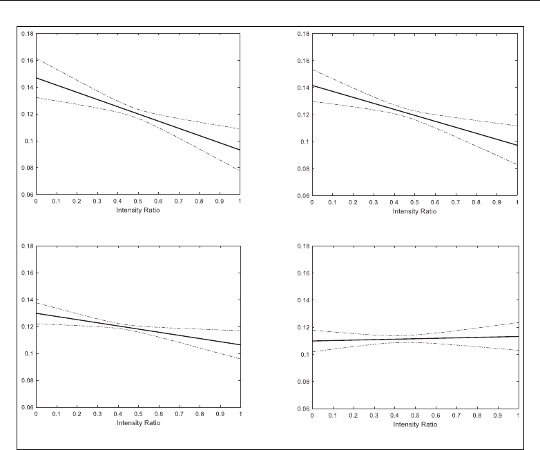
an intensity at either end of the empirical

distribution – specifically at the 1st and 99th

percentiles. Across all zones, the 1st and

99th percentiles of the intensity ratio are

0.103 and 0.705 (see Table 1). The model

implies that Zone 4 properties at the 1st per-

centile appreciated by 14.1% on average,

whereas properties at the 99th percentile

appreciated by 10.9%.

Next, we consider Zone 1, which permits

the least site development and is the quasi-

control. The coefficient on intensity is close

to zero, which implies very little variation in

expected house price appreciation condi-

tional on intensity, varying between 11.0%

(intensity = 0) and 11.3% (intensity = 1).

The difference in appreciation rates at the

1st and 99th percentiles of intensity is smaller

(11.0% versus 11.2%).

The difference in appreciation rates

between Zone 4 (upzoned) and Zone 1 (non-

upzoned) reveals how the price impact of

upzoning depends on intensity. This differ-

ence is depicted in Supplemental Figure A4.

Notably, houses in Zone 4 with intensity

above 0.63 (the 95th percentile) depreciated

when compared with houses in Zone 1 with

intensity above 0.63. This implies that

upzoning decreased prices on pre-existing

high intensity housing. Conversely, houses

Terrace Housing and Apartments (Zone 4) Mixed Housing Urban (Zone 3)

Mixed Housing Suburban (Zone 2) Single House (Zone 1)

Figure 2. Expected price appreciation conditional on intensity ratio and residential zone.

Notes: Conditional expectations are based on OLS estimation of (3). See Table 2 for estimated coefficients. Dashed lines

represent 95% confidence intervals. Standard errors are robust to spatial dependence and heteroscedasticity.

970 Urban Studies 58(5)

in Zone 4 with intensity below 0.63 appre-

ciated relative to houses in Zone 1 with

intensity below 0.63, implying that upzoning

increased prices of moderate and low inten-

sity housing.

Predicted price changes in Zones 2 and 3

further corroborate the predictions of the

real option model. Houses located in Zone 3

(which permits more development than

Zones 1 and 2, but less than Zone 4) appre-

ciated by between 14.1% (intensity = 0) and

9.7% (intensity = 1). Corresponding figures

at the 1st and 99th percentiles are 13.7% and

11.1%. Houses located in Zone 2 (which per-

mits more development than Zone 1, but less

than Zones 3 and 4) appreciated by between

13.0% (intensity = 0) and 10.6% (intensity =

1) per year. Corresponding figures at the 1st

and 99th percentiles are 12.7% and 11.3%.

A consistent pattern emerges. The impact

of upzoning on prices diminishes as intensity

increases. Beyond a sufficiently high inten-

sity, the upzoned property depreciates rela-

tive to similar properties that were not

upzoned.

The statistically significant controls also

merit brief comment. House price apprecia-

tion is decreasing in distance to downtown

(perhaps reflecting increased congestion

costs), increasing in building age, and increas-

ing in number of bathrooms (consistent with

the well-documented increase in population

pressures in Auckland over the sample

period). Interestingly, however, after condi-

tioning other controls, including the number

of bedrooms and bathrooms, larger homes

appreciated by less over the sample period.

One potential drawback of our approach

is that we do not take into account the resi-

dential zone of the transacted house prior to

the AUP implementation.

For example,

houses rezoned to Terrace Housing and

Apartments may have already been in areas

that permitted intensive development.

However, there is no statistically significant

difference in either the average population

densities across the four zones in our sample

of transactions, suggesting that this is

unlikely.

Robustness checks

Including properties with joint land ownership. We

expand the sample to include properties that

have joint ownership of the underlying land

on the title, which includes apartments and

houses on cross-leased sites. We alter the

empirical specification slightly by including

dummy variables for properties with exclu-

sive land ownership

and for dwellings iden-

tified as apartments. Results are reported in

columns (D) through (F) of Table 2.

Our main findings are unaffected. First,

the coefficients on intensity interacted with

the upzoning treatments are negative and

statistically significant. Second, price appre-

ciation is decreasing in site intensity:

Supplemental Figure A3 shows that pre-

dicted price appreciations (by residential

zone and conditional on intensity) are very

similar to those exhibited in Figure 2.

However, the fitted model implies that a

larger proportion of upzoned houses

decreased in value relative to houses that

were not upzoned, with houses with intensity

above 0.55 (the 80th percentile) depreciating

when located in Zone 4 compared with Zone

1 (see Figure A4, available online). This is

unsurprising given that many of the dwell-

ings with joint land ownership are high

intensity (units and apartments) and further

corroborates upzoning having an immediate

depreciative effect on high intensity

dwellings.

Alternative pre- and post-treatment periods. We

also explore the extent to which our results

are sensitive to the selected pre-treatment

Greenaway-McGrevy et al. 971

and post-treatment periods. We consider

three different designs. The first examines

whether market participants anticipated

which areas would be targeted for upzoning

soon after the Local Government Act of

2010 required AC to generate a new unified

set of LURs (see section ‘Institutional back-

ground’), using 2007 to 2009 as the pre-

treatment period. The second examines

whether our findings are robust in a larger

sample that uses 2007 to 2012 as the pre-

treatment period. The third examines

whether houses prices adjusted immediately

after the draft AUP announcement in

March 2013, using 2014 to 2017 as the post-

treatment sample.

Columns (A) through (C) in Table A3

(available online) exhibit the results. Our

qualitative conclusions remain the same. The

coefficients on the upzoning dummies inter-

acted with intensity are negative and statisti-

cally significant at the 1% level (except in

two cases). Interestingly, the coefficient on

intensity is negative and statistically signifi-

cant when 2007 to 2009 is the pre-treatment

period, perhaps indicating that the redeve-

lopment premium was increasing across the

city as a whole over this longer sample

period.

Treatment spillovers. Upzoning may have real-

located development from non-upzoned to

upzoned areas, resulting in a demand spil-

lover that would cause our estimates to over-

state the price effects of upzoning. A

standard approach to control for spillovers

in difference-in-differences is to exploit var-

iation in the geographic distance between

treatment and control areas under the

assumption that the magnitude of the spil-

lover decreases with distance (Clarke, 2017).

We implement two robustness checks based

on this principle. We describe our main find-

ings below, but specific details and results

from the methods can be found in the

Supplemental Material.

First, we estimate the baseline regression

using a ‘doughnut’ sample.

The control

group consists only of Single House transac-

tions in townships that are located far from

the urban core of Auckland. These town-

ships contain no, or very little, land that has

been upzoned and thus are not subject to

the confounding demand-shifting spillover

within the township. Meanwhile, we restrict

our treatment sample to upzoned areas

within the urban core of Auckland. We find

that price appreciation rates conditional on

intensity are statistically indistinguishable

from those obtained from the baseline sam-

ple, suggesting that these spillover effects are

negligible, if present. Refer to Figure A6 and

the associated discussion in the

Supplemental Material.

Second, we implement the Clarke (2017)

method by constructing an indicator for con-

trol group (i.e. Single House) transactions

that are within a specified distance to a treat-

ment area. This proximity control dummy is

then included in the baseline regression and

is also interacted with intensity, so that the

upzoning treatment is measured relative to

control group observations that exceed the

specified distance to treatment areas. We use

both the 80th and 90th percentile distances

between Single House transactions and

upzoned areas as distance cut-offs, leaving

20% and 10% of the control sample, respec-

tively, to identify the treatment effects. The

regression results indicate no spillover effect.

Specifically, the proximity control dummy

indicator and the dummy interacted with

intensity are both statistically insignificant,

indicating that there is no statistical evidence

of a differential treatment effect between

proximate treatment and control groups

relative to distant treatment and control

groups. See Supplemental Table A5.

Placebo tests. We apply the placebo test pro-

posed by Chetty et al. (2009) by estimating

the same model over pre- and post-treatment

972 Urban Studies 58(5)

periods that altogether precede the AUP

announcement. These placebo tests serve

two purposes. First, they indicate whether

geographic variation in upzoning is related

with any omitted variables driving long-run

variation in house prices. Second, they tell us

whether the upzoning treatment was antici-

pated by the market prior to the draft AUP

announcement in 2013.

We focus on three placebo pre- and post-

treatment periods: 2005 to 2007 (pre) and

September 2011 to 2012 (post); 2004 to 2006

(pre) and September 2010 to 2011 (post);

and 2003 to 2005 (pre) and September 2009

to 2010 (post). These dates mimic the pre-

and post-treatment structure used in our

preferred specification, but the relevant peri-

ods have been pushed back in time by

between 5 and 7 years, so that the first draft

AUP announcement in March 2013 is

omitted altogether from the sample periods.

Columns (D) through (F) in Supplemental

Table A3 exhibit the results.

In all placebo samples the coefficients

on the upzoning dummies are mostly statis-

tically insignificant. The single exception is

the coefficients on the Zone 3 dummies in

the 2003–2005 to September 2009–2010

sample, which are significant at the 5%

level but incorrectly signed. From this we

may conclude that there is no d ifferential

effect of intensity on house price inflation

across the four zones prior to the draft

AUP announcement in 2013. This suggests

that the geographic variation in upzoning

is unrelated to any omitted variables driv-

ing l ong-run variation in house prices, and

that the market did not anticipate which

areas would be u pzoned prior to the first

announcement.

Conclusion

This paper examines the short-run impact

of a large-scale upzoning on house prices

and redevelopment premiums in Auckland.

Upzoning unambiguously increases redeve-

lopment premiums, as predicted by real

option theory, but the net effect of the policy

on house prices is mediated by the property’s

economic potential for site redevelopment,

with less-developed properties appreciating

relative to intensively developed properties.

These findings passed several robustness

checks and placebo tests.

Upzoning is increasingly advocated and

implemented in response to unaffordable

housing (Freeman and Schuetz, 2017;

National Public Radio, 2019), and our find-

ings have important implications for evalu-

ating the efficacy and impacts of upzoning

programmes. First, policy evaluation should

primarily be based on prices of targeted

intensive housing forms (apartments and

terraced housing), not those of underdeve-

loped, single house properties that are likely

to appreciate from upzoning. Second, there

are immediate distributive impacts of upzon-

ing on wealth within the population of

home-owning households, with owners of

underdeveloped properties realising an

increase in wealth relative to owners of

intensively developed properties.

We also find that properties that exceeded

a sufficiently high level of development

depreciated relative to similar non-upzoned

properties, indicating that upzoning can

have an immediate depreciative effect on

pre-existing high intensity housing.

Although this is consistent with the market

anticipating future construction of intensive

housing, concerns remain regarding the

capacity for upzoning to generate an

increase in construction sufficient to signifi-

cantly reduce house prices (Favilukis et al.,

2019) or improve housing affordability for

middle and lower income households

(Rodriguez-Pose and Storper, 2020;

Wetzstein, 2019). Thus, the long-run impact

of the AUP on house prices and affordabil-

ity hinges on a variety of additional factors

that merit further investigation. This

Greenaway-McGrevy et al. 973

includes the amount of intensive housing

construction generated; the pricing composi-

tion of that housing; distributional impacts

on housing accessibility and home owner-

ship across socioeconomic groups; and the

intersection and coordination of zoning with

urban transportation and development poli-

cies. These areas are beyond the scope of

this paper but are worthy potential future

research topics.

Acknowledgements

We thank Andrew Coleman, Arthur Grimes,

Jyh-Bang Jou, Will Larson, Kirdan Lees, Peter

Nunns, Chris Parker, Peer Skov, and seminar

participants at the Auckland University of

Technology, Otago University, the 2018 NZAE

meetings, and the joint MBIE Treasury workshop

in urban economics for helpful comments. We

thank Corelogic New Zealand for providing the

residential transaction dataset.

Author note

A previous version of this paper was circulated as

Greenaway-McGrevy R, Pacheco G and Sorensen

K (2018) Land use regulation, the redevelopment

premium and house prices. Working Paper 2018-02,

Auckland University of Technology, Department of

Economics.

Declaration of conflicting interests

The author(s) declared no potential conflicts of

interest with respect to the research, authorship,

and/or publication of this article.

Funding

The author(s) disclosed receipt of the following

financial support for the research, authorship, and/

or publication of this article: This work was sup-

ported in part by the Marsden Fund Council from

government funding, administered by the Royal

Society of New Zealand, under grant No. 16-

UOA-239. Sorensen gratefully acknowledges the

support of the Kelliher Trust PhD Scholarship.

ORCID iD

Ryan Greenaway-McGrevy https://orcid.org/

0000-0002-2822-9849

Notes

1. Freemark (2019a: 5) states: ‘Schill noted in

2005 that there has been insufficient study

of the effects of land use reforms on housing

supply and values, and that remains true

today’.

2. Freeman and Schuetz (2017: 229) state ‘[T]o

date no city has systematically upzoned large

shares of land as a mechanism to promote

affordability’.

3. Two elements of the AUP were not fully

operational at this time: (1) parts subject to

Environment Court and High Court under

the Local Government Act 2010, and (2) the

regional coastal plan of the PAUP, which

required Minister of Conservation approval.

4. Prior to the AUP, with infill and redevelop-

ment there was estimated capacity for

345,176 additional dwellings (Fredrickson

and Balderston, 2013: 15). After the AUP,

this figure was 1,076,267 (Auckland Council,

2017: 38).

5. DiNardo (2008) explains that quasi-natural

experiments are ‘serendipitous situations in

which persons are assigned randomly to a

treatment (or multiple treatments) and a

control group’, which permit analysis of out-

comes with respect to the particular treat-

ment. In our setting, the unit of observation

are properties and the treatment is upzoning.

6. AUs are non-administrative geographic

areas defined by Statistics NZ. Within resi-

dential urban areas, AUs are typically a col-

lection of city blocks or suburbs and contain

3000–5000 persons. For additional details

see http://aria.stats.govt.nz/aria/#Classifi

cationView:uri=http://stats.govt.nz/cms/

ClassificationVersion/cVYnMpeILgJRAY7E

7. Cross-leasing was an inexpensive alternative

to subdivision in NZ, whereby two or more

title holders jointly own the land underlying

the residential structures and lease use of the

land back to one-another at a peppercorn

rate.

974 Urban Studies 58(5)

8. AUP geographic vector data obtained from

the Department of Geography, University of

Auckland.

9. Because we only have the decade in which

the house was built, ages are approximated

based on the first year of the decade.

10. We use the location of the iconic ‘Skytower’.

11. 2006 census data. The next census is in 2013,

which is during the observation period.

Median incomes above NZ$100,000 are

truncated to NZ$100,000 for 19 of the

approximately 340 AUs.

12. We also considered the distance to the near-

est rail, ferry or express busway station

instead of distance to downtown. Our main

findings were unaffected but model fit

reduced marginally.

13. There was no uniform set of planning rules

for the region. Prior to amalgamation (see

section ‘Institutional background’) the seven

authorities used different plans, resulting in

approximately 99 residential zones.

14. Results not reported for brevity but are

available upon request.

15. The dummy is effectively interacted with

(log) land area because our dataset only has

land area for houses with exclusive owner-

ship of land on the title.

16. Without information on the entire stock of

dwellings we cannot use the model to esti-

mate the proportion of housing that

decreased in relative price from upzoning.

However, the model implies that 26.9%,

1.74% and 0.38% of the transacted houses

in Zones 4, 3 and 2, respectively, experienced

a decrease. However, selection effects mean

that this sample of transacted houses is

unlikely to be representative of Auckland’s

housing stock.

17. We thank an anonymous referee for suggest-

ing this approach.

References

Anacker KB (2019) Introduction: Housing

affordability and affordable housing. Interna-

tional Journal of Housing Policy 19(1): 1–16.

Atkinson-Palombo C (2010) Comparing the capi-

talisation benefits of light-rail transit and over-

lay zoning for single-family houses and

condos by neighborhood type in Metropolitan

Phoenix, Arizona. Urban Studies 47(11):

2409–2426.

Auckland Council (2017) National policy state-

ment on urban development capacity 2016:

Housing and business development capacity

assessment for Auckland. Auckland: Auck-

land Council. Available at: https://knowledge-

auckland.org.nz/publications/national-policy-

statement-on-urban-development-capacity-

2016-housing-and-business-development-

capacity-assessment-for-auckland/

Balderston K and Fredrickson C (2014) Capacity

for Growth Study 2013 (Proposed Auckland

Unitary Plan): Results. Auckland Council

technical report, TR2014/010. Auckland:

Auckland Council.

Been V, Ellen IG and O’Regan K (2019) Supply

skepticism: Housing supply and affordability.

Housing Policy Debate 29(1): 25–40.

Chakraborty A, Knaap G-J, Nguyen D, et al.

(2010) The effects of high-density zoning on

multifamily housing construction in the sub-

urbs of six US Metropolitan areas. Urban

Studies 47(2): 437–451.

Chetty R, Looney A and Kroft K (2009) Salience

and taxation: Theory and evidence. American

Economic Review 99(4): 1145–1177.

Clapp JM and Salavei K (2010) Hedonic pricing

with redevelopment options: A new approach

to estimating depreciation effects. Journal of

Urban Economics 67(3): 362–377.

Clapp JM, Jou J-B and Lee T (2012a) Hedonic

models with redevelopment options under

uncertainty. Real Estate Economics 40(2):

197–216.

Clapp JM, Salavei Bardos K and Wong SK

(2012b) Empirical estimation of the option pre-

mium for residential redevelopment. Regional

Science and Urban Economics 42(1): 240–256.

Clarke D (2017) Estimating difference-in-

differences in the presence of spillovers. Munich

Personal RePEc Archive (MRPA) Working

Paper 81604. Available at: https://mpra.u-

b.uni-muenchen.de/81604/

Conley TG (1999) GMM estimation with cross

sectional dependence. Journal of Econometrics

92(1): 1–45.

Dalton M and Zabel J (2011) The impact of mini-

mum lot size regulations on house prices in

Greenaway-McGrevy et al. 975

Eastern Massachusetts. Regional Science and

Urban Economics 41(6): 571–583.

Demographia (2018) 15th Annual Demographia

International Housing Affordability Survey.

Available at: http://demographia.com/dhi2019.

pdf

DiNardo J (2008) Natural experiments and quasi-

natural experiments. In: Macmillan Palgrave

(ed.) The New Palgrave Dictionary of Econom-

ics. London: Palgrave Macmillan.

Favilukis J, Mabille P and Van Nieuwerburgh S

(2019) Affordable housing and city welfare.

NBER Working Paper 25906. Cambridge,

MA: National Bureau of Economic Research.

Fredrickson C and Balderston K (2013) Capacity

for Growth Study 2012. Working Report,

Auckland Council. WR2012/006. Auckland:

Auckland Council. Available at: https://

www.aucklandcouncil.govt.nz/plans-projects-

policies-reports-bylaws/our-plans-strategies/

unitary-plan/history-unitary-plan/documents-

section32reportproposedaup/appendix-3-4-

8.pdf

Freeman L and Schuetz J (2017) Producing

affordable housing in rising markets: What

works? Cityscape: A Journal of Policy Devel-

opment and Research 19(1): 217–236.

Freemark Y (2019a) Upzoning Chicago: Impacts

of a zoning reform on property values and

housing construction. Urban Affairs Review

56(3): 758–789.

Freemark Y (2019b) Doubling housing produc-

tion in the Paris region: A multi-policy, multi-

jurisdictional response. International Journal

of Housing Policy. Epub ahead of print 19

December 2019. DOI: 10.1080/19491247.

2019.1682233

Gabbe CJ (2018) Why are regulations changed?

A parcel analysis of upzoning in Los Angeles.

Journal of Planning Education and Research

38(3): 289–300.

Glaeser EL and Gyourko J (2003) The impact of

building restrictions on housing affordability.

Economic Policy Review 9(2): 21–39.

Glaeser EL and Ward B (2009) The causes and

consequences of land use regulation: Evidence

from Greater Boston. Journal of Urban Eco-

nomics 65(3): 265–278.

Gyourko J and Molloy R (2015) Regulation and

housing supply. In: Duranton G, Henderson

JV and Strange WC (eds) Handbook of

Regional and Urban Economics. Vol. 5 of

Handbook of Regional and Urban Economics.

Amsterdam: Elsevier, pp. 1289–1337.

Hilber CA and Vermeulen W (2016) The impact

of supply constraints on house prices in Eng-

land. The Economic Journal 126(591): 358–405.

Ihlanfeldt K (2007) The effect of land use regula-

tion on housing and land prices. Journal of

Urban Economics 61: 420–435.

Jackson K (2016) Do land use regulations stifle resi-

dential development? Evidence from California

cities. Journal of Urban Economics 91: 45–56.

Manville M, Monkkonen P and Lens M (2020)

It’s time to end single-family zoning. Journal

of the American Planning Association 86(1):

106–112.

National Public Radio (2019) How U.S. cities are

tackling the housing affordability crisis. Avail-

able at: https://www.npr.org/2019/08/28/

755113175/1a-across-america-how-u-s-cities-

are-tackling-the-affordable-housing-crisis

(accessed 10 September 2019).

O’Flaherty B (1994) Land assembly and urban

renewal. Regional Science and Urban Econom-

ics 24(3): 287–300.

Pogodzinski JM and Sass TR (1991) Measuring

the effects of municipal zoning regulations: A

survey. Urban Studies 28(4): 597–621.

Quigley JM and Raphael S (2005) Regulation and

the high cost of housing in California. Ameri-

can Economic Review 95(2): 323–329.

Rodriguez-Pose A and Storper M (2020) Hous-

ing, urban growth and inequalities: The limits

to deregulation and upzoning in reducing eco-

nomic and spatial inequality. Urban Studies

57(2): 223–248.

Schill MH (2005) Regulations and housing devel-

opment: What we know. Cityscape: A Journal

of Policy Development and Research 8(1): 5–20.

Wetzstein S (2019) Assessing post-GFC housing

affordability interventions: A qualitative

exploration across five international cities.

International Journal of Housing Policy.Epub

ahead of print 30 October 2019. DOI:

10.1080/19491247.2019.1662639

976 Urban Studies 58(5)