
Understanding the “Whys”
Behind Juvenile Crime Trends
Grantee: University of Pennsylvania
Award Number: 2001-JN-FX-K001
1993 1994 1995 1996 1997 1998 1999 2000 2001 2002 2003
November 2012

Understanding the “Whys” Behind Juvenile Crime Trends
1
Preface
In 2001, the Office of Juvenile Justice and Delinquency Prevention (OJJDP) funded a multiyear
project called “Understanding the ‘Whys’ Behind Juvenile Crime Trends.” It was designed to examine
the various explanations offered for the drop in juvenile crime during the 1990s and to assess how
useful they were in developing leading indicators of future trends. More specifically, the project had
three distinct but related goals:
1. To better understand the national downturn in most measures of juvenile crime, which, for
most types of crime, began around 1993 following a large increase during the preceding 7
years;
2. To work with local jurisdictions to incorporate valid explanations and correlates into a tool
that could be applied to data they already collect, so they could monitor leading indicators
of future turning points in their juvenile crime trends; and
3. To disseminate to the juvenile justice field both a better understanding of juvenile crime
trends and the leading-indicator tools developed with the local partners.
This effort was complemented by a series of ongoing, supplemental research projects intended to
fill gaps in knowledge that could prove important to predicting juvenile crime.
In one study, Fabio and colleagues (2006) measured age, period, and cohort effects on the
association and time lag between precursor risky behaviors (e.g., school truancy) and serious juvenile
offending. In another, Weisburd and colleagues (2009) used Seattle data to address two questions: (1)
neighborhood trajectories of violent juvenile crime (Groff et al., 2009), and (2) the concentration of
juvenile crime in locations as small as street blocks and the influence of those locations on jurisdiction-
level trends in juvenile crime (Weisburd et al., 2007). The Seattle results also will be reported in a future
OJJDP Research Bulletin.
Additional research that contributed to this book included the following: Souryal-Shriver’s review
of published research on causes and correlates of juvenile crime; analyses by Koper and Daly of trends
in community characteristics, criminal and juvenile justice practices, and juvenile crime during the
1990s in large cities and counties; Lynch and Snyder’s analysis of the interplay between juvenile drug
dealing and other forms of economic crime by juveniles; and Huizinga’s analysis of Denver data to
measure the extent to which trends in known causes and correlates of juvenile crime may explain
jurisdiction-level juvenile crime trends.
Finally, two future papers by Koper, Shelley, and Roth will report the results of attempts to forecast
juvenile crime trends in Los Angeles and Philadelphia.
The authors gratefully acknowledge OJJDP’s financial support of this work through Grant #2001-
JN-FX-K001. The findings and opinions expressed in this report are those of the authors and do not
necessarily represent the official position or policy of OJJDP. We are extremely grateful for the advice
and assistance of two OJJDP grant monitors: Barbara Allen-Hagen, who began the project; and Janet
Chiancone, who saw it through to completion. The work of the researchers named above contributed
immeasurably to the quality of the study. We are also grateful to the following individuals who served
as advisors to the project in its early stages: David Farrington, David Huizinga, John Laub, Rolf Loeber,

Understanding the “Whys” Behind Juvenile Crime Trends
2
James Lynch, Doris McKenzie, Howard Snyder, David Weisburd, and Charles Wellford. The authors,
however, are solely responsible for all errors and omissions in this report.

Understanding the “Whys” Behind Juvenile Crime Trends
4
Chapter 1: The Whys of the Project
By examining national trends in serious violence, one gains a better understanding of why juvenile
crime dropped so dramatically during the 1990s and remained relatively low for at least a decade.
While most would agree that the decrease actually occurred, there still are those who contend that the
drop (or its continuation) is largely an artifact of manipulation of crime statistics by some police
departments and the Federal Bureau of Investigation (FBI) (Karmen, 2000). Measuring the decrease
through multiple lenses should put this speculation to rest.
Disaggregating overall trends in serious juvenile crime informs the use of more rigorous analytical
methods for identifying and isolating factors that preceded or accompanied the drop in crime. To the
extent that the decrease was greater for some types of crime than others, greater among some
populations, or greater in some specific places, that helps narrow the range of possible explanations. If
the crime drop occurred disproportionately in large central cities, for example, then the search for
explanations could focus on those places and determine what it is about them that could have
precipitated their more pronounced decreases. Finally, the crime trends can be used to check on the
adequacy of the explanations emerging from more sophisticated analysis. Factors identified from
theory and more fine-grained analysis as the likely causes of crime drop must be shown to fit the
national crime trends during that period. That is, these factors must be shown to (1) have a likely effect
on crime; (2) be of sufficient magnitude or prevalence that changes in them could account for a
substantial portion of the drop; and (3) be distributed in the population, over time, and across places
in a manner that would account for the observed trends. The description of crime trends presented
here, then, will not only suggest where to look for explanations but also test whether the factors
identified in other analyses could have produced the decreases observed.
The intent of this project is to meet a specific need in juvenile justice policy analysis rather than
provide a comprehensive review of all scientific literature on causes of juvenile crime.
This book has five chapters, Chapters 2–5, which will be summarized in the remainder of this
chapter:
Chapter 2 establishes the groundwork for the subsequent three, using data from the National
Crime Victimization Survey (NCVS) and the Uniform Crime Reports (UCR) to describe Nation-
level trends in serious juvenile crime.
Chapter 3 accounts for trends in measurable conditions and processes in communities which,
combined, contribute to national trends in serious and violent juvenile delinquency.
Chapter 4 focuses primarily on the cultural processes that influence families and, in turn,
children’s involvement in delinquency. It examines both risk and protective cultural factors
related to family, school, religiosity, the legitimacy of the criminal justice system, violence in the
media, use of firearms, and gang membership.
Chapter 5 includes evaluations of the impact of various public policies and practices on
juvenile crime trends.

Understanding the “Whys” Behind Juvenile Crime Trends
5
Overview of Chapter 2
Lynch and Snyder report that UCR arrest counts and NCVS victimization counts provide consistent
accounts of national trends in serious violent juvenile crime (i.e., homicide, rape, robbery, and
aggravated assault) between 1980 and 2000.
Figure 1-1. Juvenile Arrest Rate for Serious Violence, 1980–2004
Figure 1-1 displays annual UCR juvenile arrest rates for violent crimes for the period 1980–2000.
The rate hovered around 300 arrests per 100,000 juveniles from 1980 through 1987, when it began
rising steadily to a peak at about 530 in 1993. The trend reversed at that point; by 2000, the rate had
returned to about 300 arrests per 100,000, where it remained for the next several years.
0.0
100.0
200.0
300.0
400.0
500.0
600.0
700.0
800.0
1980
1981
1982
1983
1984
1985
1986
1987
1988
1989
1990
1991
1992
1993
1994
1995
1996
1997
1998
1999
2000
2001
2002
2003
2004
Years
Rates per 100,000 persons age 12-17
Violent Crime Index

Understanding the “Whys” Behind Juvenile Crime Trends
6
Figure 1-2. Serious Violent Offending Rates for Juveniles and Youth Adults with and
without Adult Co-offending, 1980–2004
Figure 1-2 shows that, over the same period, the NCVS rate of violent victimizations perpetrated by
at least one juvenile offender mirrored the juvenile arrest trend. In 1982, the offending rates for
juveniles and for 18- to 29-year-olds were both about 6,000 offenses per 100,000. However, by 1993,
the juvenile rate had approximately doubled to 12,000, while the young-adult rate remained just
below 6,000. At that point, both rates began falling. However, because the juvenile drop was so much
steeper, both rates were below 4,000 offenses per 100,000 by the year 2000.
When the overall trend is disaggregated by demographics and type of crime, specific patterns
emerge that serve as a starting point for understanding the increase and following decrease in serious
violent offending among juveniles. First, the trends in violent crime were more pronounced for
juvenile offenders than for adults. This was true for both the increase in crime between the mid-1980s
and 1993 and the drop in crime in the mid-1990s. This trend was similar but attenuated for young
adults, but not for older adults. This finding suggests that the factors driving the drop in crime are
significantly more pronounced in the juvenile and young-adult populations. Furthermore, the increase
in overall serious violent offending in the 1980s was not concentrated among black youth, with the
exception of homicide. However, the decrease in serious violent offending in the 1990s was greater for
black than for white youth.
Because males commit most violent crimes, it is not surprising that the male trends between 1980
and 2000 resemble the inverted U shape seen in overall trends. In contrast, violent female offending
rose throughout the entire period, doubling between 1980 and 2000. Female offending, however,
represents such a small percentage of serious and violent offending that it had little impact on
national crime trends.
The risk factors of an urban environment also figure prominently in many explanations of serious
and violent juvenile offending. For example, Blumstein and Wallace (2000) found that the 20 largest
0
2000
4000
6000
8000
10000
12000
14000
1980
1981
1982
1983
1984
1985
1986
1987
1988
1989
1990
1991
1992
1993
1994
1995
1996
1997
1998
1999
2000
2001
2002
2003
2004
Years
Rates per 100,000
<18 (1) 18-29 (1)
All <18 (2)
18-29 (2)

Understanding the “Whys” Behind Juvenile Crime Trends
7
cities in the United States account for 80 percent of juvenile homicides. However, serious violent
juvenile offending decreased during the 1990s not only in central cities, but also in suburban and rural
areas. Therefore, the explanation for the crime drop should not be focused solely on urban
environments.
Finally, the data show that between 1980 and 2000, patterns of offending by juveniles were
changing in several ways. During the overall crime drop in the 1990s, there were especially large
decreases in group offending, juvenile co-offending with adults, use of firearms, and stranger-on-
stranger offending. And patterns in drug offending and serious violent offending among juveniles
varied significantly based upon the race of the offender. For white juveniles, increases in drug arrests
were associated with decreases in arrests for serious violent offending. In contrast, for black juveniles,
decreases in drug arrests were associated with decreases in arrests for serious violent offending. This
difference is difficult to interpret. It may suggest a deterrent effect of drug arrests on serious violent
offending for white but not for black juveniles. But it may merely reflect police patrolling patterns:
more intensive patrolling in largely black neighborhoods may increase the chances that both drug
and violent offenses are discovered and followed by arrests.
Criminologists, criminal and juvenile justice practitioners, public health professionals and others all
have attempted to explain the national juvenile crime trends described above. The following chapters
examine many of the conditions and processes they have offered from two perspectives: (1) evidence
that they affect criminal behavior, and (2) evidence that their patterns and trends from 1980 to 2000
were consistent with juvenile crime trends during the 1990s.
Overview of Chapter 3
Chapter 3 considers community- and neighborhood-level characteristics and processes that may
combine to influence national trends. Five categories are examined: (1) the proportion of the
population in demographic categories that are most at risk for offending; (2) the extent and
concentration of poverty in a community; (3) the prevalence of dysfunctional family structures; (4)
social organization and informal social control; and (5) employment opportunities.
Criminologists generally agree that age and gender are two of the most important correlates of
criminality. Rates of crime escalate and peak during adolescent years and taper off as the individual
ages (e.g., Ezell & Cohen, 2005; Farrington, 1986; Hirschi & Gottfredson, 1983; Sampson & Laub, 1992).
Male juveniles are responsible for a disproportionate amount of crime, and an obvious implication of
this is that the size of the male juvenile and young-adult populations should coincide with changes in
the aggregate crime rates. The empirical evidence on the size of the high-risk youth population,
however, yields mixed results (Donohue & Levitt, 2001; Easterlin, 1978, 1987; Hay & Evans, 2006;
Lauritsen, 2003). Further analysis of Census data and National Center for Health Statistics (2004) data
indicates that the male juvenile population declined slightly from 1980 to 1990 when serious and
violent crime was rising, and it rose slightly while serious and violent juvenile offending was declining
during the 1990s. As such, the relative changes in the size of the male juvenile population do not seem
to provide a strong explanation for the rise and fall in violent delinquency.
Of course, not all juveniles share the same level of risk for delinquency. Youth born to teen
mothers, growing up in communities with higher concentrations of poverty, and living in single-
parent households are at greater risk. Trends in some of these risk factors parallel the trends of the
time period 1980–2004, while others do not. For example, the birthrate of children born to teen

Understanding the “Whys” Behind Juvenile Crime Trends
8
mothers declined from 1980 to 2000, trending toward older mothers and smaller families (Orlebeke,
2001). However, the national trends for families in poverty are fairly consistent with the juvenile crime
trends. Areas with high concentration of poverty have consistently higher crime rates, and
criminologists have long documented the relationship between difficult economic conditions and
crime. Poverty rates for children and families increased between 1985 and 1992 and decreased
between 1992 and 1998. This increase and decrease was greater for black families than for non-
Hispanic white families. Although these trends do not imply causation, they make clear that the two
issues are closely linked.
Another risk factor that is difficult to disentangle from poverty is family disruption. Youth living in
single-parent households are more likely to be poor than youth living in two-parent homes (Mack et
al., 2007). The empirical evidence documents both direct and indirect links between family disruption,
poverty, and delinquency (see Campbell, Hu, & Oberk, 2006; Demuth & Brown, 2004; Lauritsen, 2003).
A high prevalence of disrupted families is thought to increase delinquency both by its effects on
children and by weakening formal and informal community social controls. A low tax base in low-
income neighborhoods provides fewer resources to local law enforcement; children are more likely to
be unsupervised and more likely to associate with delinquent peers; and feelings of mutual obligation
are reduced, making residents of disorganized communities less likely to intervene in problems of
neighborhood children. Overall, the result is a reduction in community capacity to deter crime.
Trends in the number of poor, female-headed households with children were consistent with
juvenile crime trends. They both show an increase between 1985 and 1992 and then a decrease
between 1993 and 1998. Similar to the trends documented in Chapter 2, these increases and
decreases were more pronounced for black families than for whites. Employment opportunity, or the
lack thereof; routinization of the drug trade; and changes in economic opportunity in the drug
markets are three explanations offered for the crime drop. Changes in unemployment are somewhat
consistent with the crime drop; however, the relationship between unemployment and crime is
complex, especially for juveniles. Some have argued that increases in legitimate opportunity reduce
incentives for involvement in crime, reduce the burden and stress of unemployment, and strengthen
mechanisms of social control. Conversely, others argue that unemployment may contribute to a
reduction in crime by lowering the number of empty homes during the day, and may reduce the
number of potential targets by reducing the number of individuals traveling alone with valuables in
various neighborhoods at various points in the day. Furthermore, juveniles are less invested in the
labor market than their adult counterparts. The empirical evidence is mixed. Some evidence suggests
that juveniles who are employed are more likely to be delinquent than those who are not (e.g.,
Ploeger, 1997); other studies draw the opposite conclusion (e.g., Fergusson et al., 1997).
Blumstein (1995, 2006) argues that changes in the drug market and the punitive responses of the
criminal justice system influenced the rise and fall of serious violence committed by juveniles. The
expansion of the crack market involved recruiting and arming juveniles for participation in drug sales.
Juveniles were less expensive to hire, were not subject to the same consequences, and were less risk
averse than adults. Juveniles also were more vulnerable to robbery. Therefore, arming young males
who were involved in turf wars likely contributed to the escalation in violent offending during the late
1980s. However, the combination of changes in police practices, norms resulting from addiction, and
legitimate employment opportunities in the 1990s stabilized the drug markets and thus reduced the
related violence. This hypothesis seems to be consistent with the trends described in Chapter 2.

Understanding the “Whys” Behind Juvenile Crime Trends
9
Overview of Chapter 4
Chapter 4 considers family- and individual-level conditions, which may in turn reflect cultural,
social, or biological influences. Criminologists reference multiple cultural factors—such as family
characteristics, schools, religiosity, violence in the media, use of firearms, and gang membership—in
explaining serious and violent juvenile delinquency. In the study of the influence of family factors on
delinquency, there appears to be a great deal of variation in the predictions made. First is that changes
in the demographics and the value of the familial institution influence trends in delinquency (see
Popenoe, 1993). Accordingly, the decline of family values since the 1970s should result in an upward
trend of juvenile crime. However, with the exception of changes in divorce rates, which began to
decrease when the crime drop began, this argument is inconsistent with the trends presented in
Chapter 2.
The second theoretical approach to understanding the effects of family characteristics on juvenile
delinquency is through general studies on risk and protective factors, such as the direct negative
relationship between parental monitoring and delinquency. The third explanation involves the idea
that family characteristics are multidimensional, and so the effects of different family variables should
be distinguished from one another. For example, family size and structure are related to delinquency
but are moderated by parental monitoring, family conflict, family substance abuse, and family
members’ criminal backgrounds. Family size and structure indirectly influence delinquency through
the amount of time spent with children and the quality of familial bonds (attachment). There remains
a great deal of variation in this approach, and the patterns in this category of research are not as
simple as the patterns identified in the more general risk-and-protective-factors studies.
The trend toward smaller families influences the amount and quality of time that parents can
spend with their children. While it has been documented that children increasingly have two parents
participating in the labor force, Sandberg and Hofferth (2001) found that parents reported spending
more time with their kids when the crime drop began. It is possible that working parents begin
spending more time with their children when they are not working. While there is evidence for both
the direct and indirect effects of family characteristics on delinquency, the support for direct controls
is much stronger. One limitation of these studies, however, is that many of them focus on family
structure and process during adolescence, and little has been done on how these variables affect the
developmental process in early childhood.
Schools and religious institutions are also linked to the explanations of the juvenile crime drop in
the 1990s. Schools play an important role in the lives of adolescents; they spend most of their day in
the classroom and not only learn academics but also develop (or fail to develop) important social skills.
Variables such as attendance, positive attitudes toward school, academic achievement, aspirations,
and feeling a sense of community demonstrate negative relationships with delinquency. Much of the
research on the impact of schools on delinquency revolves around social control and changes in social
bonds (see Hirschi, 1969). However, the empirical evidence on changes in the social bonds and school
dropout rates are generally inconsistent with juvenile crime trends. On the other hand, trends in
weekly religious attendance among high school seniors are consistent with the juvenile crime trends.
Furthermore, there are noticeable differences in the magnitude of the importance of religion by race.
Throughout the 1990s, black students were more than twice as likely as white students to report that
religion played an important role in their lives. Religion is thought to decrease participation in
delinquency both directly and indirectly through belief in conventional norms, disapproval of

Understanding the “Whys” Behind Juvenile Crime Trends
10
delinquency, increased association with non-delinquent peers, and improved attachments to family
and school.
Trends of exposure to media violence also are inconsistent with the trends in juvenile crime.
Levels of violent media content did not decline during the 1990s. In fact, several scholars have
documented increases in the amount of violent content on television and in G-rated films. While
exposure to violence has been linked to aggressive and violence behavior in some people, a careful
review of the research indicates several methodological problems in many of the studies. Given the
limited empirical support for violence in the media as a causal mechanism for violence, it seems
implausible to use exposure to violent media to explain the substantial increase and decrease in
serious violent juvenile offending.
The trends in juvenile use of firearms are closely linked with gang membership, drug dealing, and
violence and parallel the crime trends in the previous two decades. There have been major changes in
arrests for possession, carrying, and use of weapons during the time period of interest here. The arrest
rate for juveniles for weapons more than doubled from the early 1980s to 1993 and then declined
sharply between 1993 and 2002. By the early 2000s juvenile homicide rates fell below the lowest point
in 1980.
There are demand- and supply-side explanations for this pattern. Blumstein argues that the
expansion and then stabilization drove juveniles’ desire to arm themselves and respond to conflict
with violence. On the supply side, changes in the production and availability of handguns are another
probable cause of the rise and fall of serious juvenile violence. Koper (2004) examined trends in
handgun production and found an increase in the production of handguns between 1987 and 1993
and a decline between 1993 and 2000. The increase in availability of handguns likely made some of
them more inexpensive, and, thus, more accessible to juveniles. However, the question of whether or
not changes in the availability of firearms to juveniles directly influence the violence level is complex.
Results from a self-report survey indicate that guns are widely available to juveniles. Therefore, it is
possible that changes in social norms, gun control laws, and punishment combined to influence or
change attitudes and behaviors regarding gun possession and use.
The trend data on the contribution of juvenile gangs to the crime trends is also somewhat unclear.
The empirical evidence demonstrates a strong and steady relationship between gang membership
and delinquency, and survey results indicate that gang members are more likely to own a gun than
non-gang members. Howell (1994) reports an increase in the number of cities citing gang problems,
and increases in gang membership and the number of gangs. The OJJDP National Youth Gang Survey
reveals a reduction in the prevalence of gangs in the 1990s (Egley & O’Donnel, 2009). These patterns
are consistent with the crime trends, especially for the greater decline in group offending than for solo
offending. However, gang data are reported by police, and they may reflect a substantial degree of
discretion in police practices in the process of identifying gang members and gang activity. While it is
difficult to draw solid conclusions, it seems plausible that fluctuations in gang membership
contributed to the crime trends described in Chapter 2.
Overview of Chapter 5
Chapter 5 considers government policies and practices that may affect crime trends either directly
(e.g., policing) or indirectly (e.g., public housing). It covers crime-control programs ranging from
prenatal care for high-risk mothers, to changes in housing policies intended to reduce the effects of

Understanding the “Whys” Behind Juvenile Crime Trends
11
concentrated poverty, to police strategies to reduce juvenile offending. The effectiveness of programs
and policies are evaluated, followed by an examination of the breadth of the implementation and
then the consistency with the juvenile crime trends. The policies are grouped into three categories:
primary prevention, secondary prevention, and other public policies that may have an indirect effect
on the juvenile crime.
Primary Prevention Strategies
Primary prevention programs seek to reduce the harm from juvenile crime by intervening in a
broad segment of the population. Chapter 5 examines the following types of primary prevention
programs: prenatal and perinatal programs designed to improve the overall health of pregnant
women, lead abatement programs and environmental policies designed to reduce young children’s
exposure to lead, lead screening programs for at-risk youth, family intervention programs for at-risk
families, preschool interventions such as Head Start, and after-school programs such as Boys and Girls
Clubs of America.
Evidence consistently supports the link between prenatal substance abuse, low birth weight, and
increased risk for later delinquency (e.g., Day, Goldschmidt, & Thomas, 2006; Farrington, 1994; Tibbetts
& Piquero, 1999). However, aggregate trends in low birth weight and prenatal substance abuse are
inconsistent with the juvenile crime trends. Between 1970 and 1980, there was a slight decrease in live
births classified as “low birth weight” and “very low birth weight.” This decrease was followed by a
steady increase for the next two decades. Similarly, the prevalence of Fetal Alcohol Syndrome (FAS)
dropped in the 1970s and then rose between 1979 and 1993. These trends run counter to the
direction expected, assuming a 12-year time lag between birth and subsequent delinquency. This
inconsistency indicates that the proliferation of programs to improve prenatal care and substance
abuse was not a likely factor driving the crime drop of the 1990s.
Another primary prevention strategy that could plausibly be related to the juvenile crime trends is
the attempt to reduce young children’s exposure to lead, as both Federal and local policies have
aimed to do. Consistent evidence links the neurotoxic effects of young children’s exposure to lead and
increased risk for juvenile offending (e.g., Denno, 1993; Narag, Pizarro, & Gibbs, 2009; Needleman et al.,
1996). During the 1990s the Environmental Protection Agency (EPA) made a series of changes to
gasoline regulations, which reduced the concentration of lead in gasoline. The policy changes reduced
exposure to lead in a way that is consistent with the juvenile crime drop; however, it seems unlikely
that the trends in gasoline lead concentration could account for the qualitative changes in violent
juvenile offending. The regulatory changes also do not explain the increase in juvenile violence in the
1980s.
Another source of exposure to lead that is more difficult to assess is lead in house paint. Interior
paint is durable and permanent. The concentration of lead in interior house paint changed
dramatically in the 1970s, dropping from about 50 percent concentration in the 1950s to a standard of
1 percent in 1971, and even further, to 0.06 percent, in 1977. It is possible that a reduction in the
concentration of lead in house paint is related to the juvenile crime trends of the 1990s, but the link
has not been closely studied.
The research on interventions for high-risk families is generally positive (e.g., Sherman et al., 1998).
But because there are no national data on the prevalence of family intervention programs, it is not
possible to formally assess the impact of these programs on the juvenile crime drop. Furthermore, the

Understanding the “Whys” Behind Juvenile Crime Trends
12
abrupt nature of the rise and fall in juvenile violence makes the relationship between the proliferation
of family intervention programs and the juvenile crime trends unlikely.
Evidence on both preschool interventions and after-school programs is mixed and depends largely
upon the specific program, the target population, and the quality of the programming implemented.
One preschool program that could be related to the juvenile crime trends of the 1990s is Head Start, a
federally funded program for children 3 to 5 years of age. Using a 10-year lag between participation in
Head Start and involvement in juvenile delinquency, we would expect to see a decrease in enrollment
in Head Start from 1975 to 1983. Yet enrollment numbers rose from 1975 to 1989 (from 349,000 to
450,970), and they continued to increase between 1989 and 2001 (Head Start Bureau, 2002). While the
Head Start enrollment data do not correlate strongly with the juvenile crime trends, it is plausible that
the increase in Head Start enrollment had a small impact on juvenile violence during the 1990s.
After-school programs have gained popularity for many reasons—they provide structured
activities, academic programming, opportunities for community involvement, and, most importantly,
adult supervision during the after-school hours when many parents are working. From 1985 to 1997,
the percentage of two-parent families with children with both parents participating in the labor force
rose from 59 percent to 68 percent (Bureau of Labor Statistics, 2009). Despite their popularity, most
evaluations of the impact of after-school programs on delinquency show mixed results. The paucity of
rigorous evaluations does not provide a great deal of theoretical support for increased after-school
programs having a strong causal impact on the juvenile crime drop of the 1990s. Despite the
questionable impact on past juvenile crime trends, local data on after-school programs may be
available in many places and could be useful in local leading indicator models to predict short-term
trends in juvenile delinquency.
Secondary Prevention Strategies
Secondary prevention strategies are programs that focus on people who already have offended
and aim to reduce the opportunities for recidivism. These programs also may attempt to prevent
crimes from occurring by intervening in situations that resemble those where crimes are likely to
occur. Secondary prevention strategies may involve interventions such as gun control, juvenile curfew,
juvenile boot camps, teen courts, transfer to adult court, and other juvenile justice interventions.
Roughly half of the largest cities in the United States had curfew laws between the late 1950s and
1980s (Ruefle & Reynolds, 1996). Juvenile curfew laws increased in popularity in the 1990s, and during
the early 1990s, 45 percent of large U.S. cities enacted new or revised curfew laws. Arrests for curfew
and loitering violations tripled between 1989 and 1998 (Ruefle & Reynolds, 1996). Although the
empirical research does not demonstrate a strong link between curfew laws and reduced juvenile
delinquency, it is possible that greater enforcement of juvenile curfew laws helped reduce serious
juvenile violence during the 1990s. It is also possible that curfew enforcement in juvenile crime “hot
spots” may be an effective tool in reducing juvenile violence, but more research linking curfew laws
and juvenile violence is necessary.
Gun control is another secondary preventive strategy that could help explain the crime drop of the
1990s. As summarized in Chapter 2, gun murders dropped from 80 percent of juvenile homicides in
1994 to 67 percent in 1999. The Federal handgun ban prohibited the sale of handguns to persons
younger than 18 years; both the Gun Free School Zone Act and the Brady Act were established in the
early 1990s. A number of states also enacted new restrictions on juvenile handgun possession and
Child Access Prevention (CAP) during the 1990s, but the research on these new laws does not show a

Understanding the “Whys” Behind Juvenile Crime Trends
13
direct negative correlation with juvenile violence. There is some indirect evidence that the reforms of
the Federal firearms licensing system may have reduced homicides in urban areas by limiting the
number of gun dealers (Wiebe et al., 2009).
In the most prominent change in state gun control legislation in the 1990s, 22 states passed “shall
issue” laws, which require law enforcement to issue a permit to carry a concealed firearm. However,
there is insufficient evidence to determine whether these laws help or harm efforts to reduce juvenile
violence (National Research Council, 2005). Other innovative efforts to crack down on illegal handgun
possession in crime hot spots, such as the Youth Crime Gun Interdiction and Boston’s Operation
Ceasefire, were put in place during the 1990s. Boston’s Operation Ceasefire reduced youth homicide
by incorporating a zero tolerance policy and focusing criminal justice resources on violent gang
members. Most of these local-level efforts were undertaken during the late 1990s, and very little
evidence links them to the juvenile crime trends. In the future, data on gun control initiatives may be
useful in developing local leading-indicator models for juvenile crime and violence.
Growth in the private-sector security industry also may have contributed to the decline in serious
juvenile crime in the 1990s. Burglar alarms, private security guards, physical restructuring of
communities, and gated communities reduce juveniles’ opportunities to commit crimes. Evidence
indicates that situational crime prevention reduces crime at the neighborhood/street level (see Taylor,
2002). Unfortunately, little systematic data are available to assess the impact of such “target
hardening” on the juvenile crime trends of the 1990s. However, data on licensing records of private
security guards, locations of burglar alarms, and gated communities and buildings may permit
researchers to examine the impact in the local leading-indicators models.
Trends in juvenile justice policies—such as judicial waiver, prosecutorial discretion policies for
transferring juveniles to adult court, and statutory exclusion—also may have influenced the juvenile
crime trends. The juvenile justice system became more formal and more punitive in the 1990s.
Increasingly juveniles were tried as adults (from 1992 to 1997, 45 states passed laws expanding or
easing the transfer of juveniles from the juvenile justice system to the adult system) (Snyder &
Sickmund, 2006). Proponents of increasing the number of juveniles transferred to adult court argue
that the effects on juvenile crime can be threefold: (1) Serious violent offenders who are incapacitated
are not free to commit new offenses; (2) juveniles who have been incarcerated are less likely to
recidivate because of harsh punishment (specific deterrence); and (3) juvenile transfer provides general
deterrence. Empirical evidence, however, suggests that transferring juveniles to the adult system has
not had the intended effect; these juveniles were in fact more likely to reoffend than youth processed
in the juvenile justice system (see Cohn & Milan, 2010; Podkopacz & Feld, 1996; Redding, 2010).
Overall, greater use of juvenile transfer in the 1990s did not reduce violent juvenile crime; rather,
increasingly waiving juveniles to adult court may have worked to counter the crime drop.
Despite the crime drop that began after 1993, the trends in the juvenile justice system show that
there was an overall increase in the number of cases adjudicated (60.7 percent more between 1990
and 2000). This was coupled with increases in the number of juveniles held in a residential facility
before and after court disposition. Finally, this punitive trend also resulted in longer sentences being
handed down. The impact of these trends on the juvenile crime drop is not clear. Empirical research on
many of these trends is contradictory. For example, one study of formal versus informal processing of
less serious delinquents indicates that the outcomes of formal processing are generally worse than
those of juveniles handled informally (Petrosino, Turpin-Petrosino, & Guckenburg 2010). Furthermore,
evidence on sentence length indicates that longer sentences do not reduce rates of recidivism

Understanding the “Whys” Behind Juvenile Crime Trends
14
(Wooldredge, 1988). The evidence on the links between juvenile custody and sentencing trends that
occurred in the 1990s are contradictory with the juvenile crime trends.
The evidence linking reentry services provided to juveniles with the 1990s crime drop is also
tenuous. Juvenile violence fell during the 1990s and early 2000s, despite the increasing number of
youth returning to communities after detention. Reentry services for juveniles were not widely
recognized as an important component of successful transition until the late 1990s, and Federal
legislation on reentry services was not established until 2003. However, data from tracking juvenile
reentry patterns could help practitioners anticipate future crime trends.
Another trend in juvenile justice services that could plausibly be linked to the drop in serious
juvenile violence in the 1990s was the establishment of teen courts and boot camps. Both gained
popularity in the 1990s. Teen courts are likely to involve other teens in the process of adjudication and
include letters of apology, community service obligations, and restitution as part of the sentence.
There are few rigorous evaluations of teen courts, but there is some evidence that suggests they have
reduced recidivism in target cities (see Butts et al., 2002). Data on the creation or termination of teen
courts may be helpful in developing local leading indicator models. The evidence on the effectiveness
of boot camps is less favorable, showing that they do not reduce recidivism relative to other types of
punishment. It is implausible that the proliferation of boot camps reduced juvenile violence in the
1990s.
The presence, activities, and use of resources by law enforcement may also be linked to the
reduction in serious juvenile violence during the 1990s. Levitt (2004) estimates a 14 percent increase in
the number of police per capita during that decade. Overall, the evidence on the impact of police
staffing on crime reduction is somewhat mixed, as it is difficult to distinguish the effect of the size of
the police force on crime from the impact of rising crime on the need for police. The evidence from
more recent and sophisticated research designs indicates police staffing may have played a role in
reducing serious juvenile violence. A study cited in the appendix of Chapter 5 indicates that growth in
police staffing accounted for an approximate 6 to 12 percent reduction in serious violence in the
1990s.
Police strategies for reducing violence may be as important as the numbers of officers in any given
city. Chapter 5 includes a systematic review of five types of police interventions: order maintenance
policing, community policing, problem-oriented policing, focused policing, and specific youth-related
interventions.
Order maintenance policing, generally considered aggressive policing, addresses the quality of
life and features a zero tolerance approach to all types of delinquency/crime. The theory
behind it is that a highly visible and vigilant police force will discourage more serious offending
while alleviating behaviors that are chronically problematic (e.g., disorderly conduct, drunk
driving, prostitution, enforcement of curfew violations, etc.). This type of policing became more
popular in the 1990s, but there is little systematic data on this approach. It is possible that order
maintenance policing may have reduced crime in large cities in the 1990s (see MacDonald,
2002).
Community policing emphasizes proactive policing strategies that involve cooperation and
communication at the community level. This approach may involve a range of activities, such
as foot patrol, neighborhood watch, the establishment of community substations, strategic
problem solving, and overall efforts to reduce signs of community disorder. The evaluation

Understanding the “Whys” Behind Juvenile Crime Trends
15
results on community policing are mixed, and there is little evidence on its role in reducing
total or juvenile crime in the 1990s. One study suggested that large cities employing
community policing strategies did not have lower crime rates or larger crime drops than other
cities not using these methods (MacDonald, 2002). Another independent research project
found that agencies with stronger community policing orientation more effectively reduced
juvenile homicide (see the results of the analysis in the appendix to Chapter 5).
Problem-oriented policing includes an analysis of the problems contributing to the patterns of
crime and disorder in the community. It also may include community policing strategies, but
this approach to problem solving does not necessarily require cooperation with local residents.
Problem-oriented policing often concentrates resources on specific locations, groups, and
types of offenders. The approach was used increasingly in the 1990s, and the data linking its
effectiveness in juvenile crime trends is somewhat mixed. Some studies indicate that this type
of policing is an effective tool for crime reduction (National Research Council, 2004; Weisburd
et al. 2010); others find little evidence for crime reduction after widespread implementation of
problem-oriented policing in large U.S. cities (MacDonald, 2002). The authors suggest that the
success of this technique may be dependent upon the problem selected and the rigor with
which the solution is implemented.
Focused policing also is directed at specific places, offenders, and types of crime (e.g.,
crackdowns on drug markets, drunk driving, and elevated patrol levels around high crime
areas) and may involve order-maintenance policing, community policing, and problems-
solving initiatives as well. A recent change includes using computer record and geographic
information to map and target crime “hot spots.” The percentage of police departments
doubled from approximately 38 percent in the early 1990s to 76 percent in the early 2000s
(Johnson & Roth, 2003). It is difficult to evaluate the impact of focused policing on the juvenile
crime trends of the 1990s because COMPSTAT emerged just as crime was beginning to decline.
Another secondary prevention strategy that may have affected the juvenile crime rates is change
in state and Federal sentencing policies. Prison populations increased dramatically during the 1990s:
150 percent between 1990 and 2000. Studies on adult offending show that prison growth reduced
crime, but the impact of this overall reduction on juveniles is difficult to assess. There is little research
on how adult incapacitation specifically influences juvenile offending. Possibly, growth in the number
of incarcerated adults decreased the number of adults available to co-offend with juveniles. On the
other hand, the harsh punishment of adult offenders provided an incentive for recruiting juveniles to
participate in the drug markets (see Blumstein, 1995; 2006). Furthermore, the long-term negative
impact of incarceration on families and communities may indicate that trends in adult incarceration
may not play a significant role in reducing serious juvenile violence.
Other Policies and Programs
Finally, other public policies, such as school management, housing programs, and advances in
emergency medicine, are examined in Chapter 5. These policies are not primarily intended to prevent
juvenile crime but have indirect relevance to juvenile offending. For example, the ability of school
teachers and administrators to maintain order on and around school grounds is related to risk factors
for delinquency. The U.S. Department of Education established Safe and Drug Free Schools and
Communities, a Federal program that received $566 million in funding to reduce drugs and violence in
communities. The research on these types of programs is mixed, but evaluation data indicate that

Understanding the “Whys” Behind Juvenile Crime Trends
16
skills training and programs that aim to reinforce behavioral norms are generally favorable. School-
based intervention programs increased in the 1990s and could have contributed to the crime drop.
Changes in the funding for public housing during the 1990s also could have indirectly influenced
the juvenile crime trends during the 1990s. In 1993, the U.S. Department of Housing and Urban
Development established a $6 billion initiative called the HOPE VI program, which gave grants to
redevelop and demolish severely distressed public housing. The program helped relocate residents
from large distressed public housing complexes in order to reduce the concentration of poverty in a
single neighborhood. HOPE VI was not implemented until the late 1990s; therefore, it seems unlikely
that it was a driving factor behind the dramatic drop in juvenile violence that began in 1994.
In addition to changes in public housing policies, innovations in the practice of emergency
medicine also could be indirectly linked to the juvenile crime trends of the 1990s. It is possible that the
proliferation of trauma centers and advancements in trauma surgery reduced the number of
aggravated assaults that resulted in death. These factors may help explain why the decrease in
juvenile homicide was larger than the decrease for other types of violent offending, but it would not
account for broader qualitative changes in juvenile violence that occurred during this period.

Understanding the “Whys” Behind Juvenile Crime Trends
17
Chapter 2. Juvenile Crime Trends and Their Implications for
Understanding
(James P. Lynch, John Jay College, New York, NY, and Howard N. Snyder, National Center for Juvenile
Justice, Pittsburgh, PA)
Introduction
Nation-level trends in serious violence are the point at which the search begins to understand why
juvenile crime (and crime generally) has dropped so dramatically in the past decade. Describing the
decrease in juvenile violence through a variety of lenses can demonstrate that the drop has indeed
occurred. While most would agree that crime has decreased in the past decade, there still are those
who contend that the drop (or its continuation) is largely an artifact of crime statistics and, more
specifically, the manipulation of those statistics by the police and the Federal Bureau of Investigation
(FBI) (Karmen, 2000). This speculation should be put to rest.
By describing these violence trends, we also will inform the use of more rigorous analytical
methods for identifying and isolating the factors that preceded or accompanied the drop in crime. To
the extent that the decrease occurs in some types of crime, among some populations or in specific
places, this will narrow the range of possible explanations. If the crime drop occurred
disproportionately in large central cities, for example, then the search for explanations can focus on
those places and determine what it is about them that could have precipitated this more dramatic
decrease in juvenile crime.
Finally, the crime trends can be used to check on the adequacy of the explanations that emerge
from more sophisticated analysis. Factors identified from theory and more fine-grained analysis as the
likely causes of the juvenile crime drop must be shown to fit the national crime trends during that
period. That is, these factors must be shown (1) to have a negative effect on crime, (2) to be of the
magnitude or prevalence that changes in them could account for a substantial portion of the drop,
and (3) to be distributed in the population and across places in a manner that would account for these
trends. The simple description of crime trends presented here, then, will both suggest where to look
for explanations and confirm that the factors identified in other analyses could have produced the
decreases observed.
Crime Statistics and Crime Trends
Describing Nation-level trends in juvenile violence, like describing unemployment and other
indicators of social well-being, is dependent on national statistical systems. These systems routinely
and systematically assess the level of crime and the change in level over time. We are fortunate to
have reasonably good statistical systems for assessing these nationally in the United States. One of
these indicators is the National Crime Victimization Survey (NCVS) conducted by the Census Bureau
under the auspices of the Bureau of Justice Statistics (BJS). The other is the Uniform Crime Reports
(UCR) compiled by the Federal Bureau of Investigation (FBI).
1
These two systems employ very different
methodologies for collecting information on crime. The NCVS is a household survey in which a
1
The FBI is implementing the National Incident Based Reporting System (NIBRS) that will provide incident-level data on crimes reported
to the police. At present, this data system does not operate in enough jurisdictions to generate national estimates.

Understanding the “Whys” Behind Juvenile Crime Trends
18
representative sample of residents of the United States is asked to report on criminal victimization. The
UCR is an administrative series in which police departments report to the FBI the offenses that come to
their attention and the arrests they make pursuant to those crimes. Using this information, the FBI
produces national estimates of reported crime.
2
These two overlapping but quite different series
provide a complementary picture of the crime problem (Lynch & Addington, 2006). The NCVS includes
crimes that the UCR omits by design or because they did not come to police attention. The FBI
includes crimes such as homicide that are not in the survey. Moreover, the kinds of distortions that
affect the NCVS are very different from those that affect the UCR. This is useful in that the two series
are unlikely to be affected by the same distortions or measurement errors and it is less likely that the
same measurement errors could drive both series down in the same period. Thus, if the two series are
showing a similar drop in crime, it is unlikely that the drop is due to measurement error or to the
conscious manipulation of these statistics.
3
The NCVS and the UCR are complementary in other ways (Biderman & Lynch, 1991; Lynch &
Addington, 2006). The UCR is an aggregate reporting system that collects jurisdiction-level counts of
crime for the vast majority of places in the United States. The NCVS collects data on only a sample of
the U.S. population, but it includes very detailed information on each crime event reported in the
survey. As a result, the UCR has greater coverage and a greater ability to provide estimates on
subnational units than the NCVS. But the NCVS can provide very detailed and disaggregated
information on the nature of crime and subgroups of the population. This permits the disaggregation
of crime rates into those for different demographic groups, regional groups, and more. Used together,
these social indicators can provide a more informative and differentiated description of the drop in
juvenile crime than either could do alone.
Generating Juvenile Crime and Offending Trends
This book focuses on trends in juvenile offending and, specifically, serious violent crime committed
by juveniles—i.e., homicide, rape, robbery, and aggravated assault. Information on juvenile offending
is typically found in the UCR arrest data on Age, Sex, Race, and Ethnic Origin (ASREO) and in the
Supplementary Homicide Reports (SHR). It is more unusual to use data on offenders provided by
victims in the NCVS to describe trends in juvenile offending, as the survey is typically used to generate
trends in victimization and not offending (Lynch, 2002). Using all of these data sources complicates
the analysis because they are all different and their differences must be taken into account in
comparing levels of crime and the trends and interpreting the differences and similarities between the
trends. Much of our current understanding of trends in juvenile crime comes from UCR’s ASREO report.
These data are jurisdiction-level counts of persons arrested grouped by the most serious offense for
which they were arrested
4
. Separate counts are provided by the age, race, and gender of the arrestee.
These data are useful for describing gross trends in specific crimes but are of limited use in
disaggregating the attributes of these crimes. Another important consideration in using arrest data is
that they reflect a conjunction of offender and police behavior. Therefore, there are potential biases
2
The term estimate refers to a set of procedures followed to produce counts and rates of crime with the UCR data. Different procedures
would yield different counts and rates.
3
The strategy of using different and complementary social indicators is not unique to the justice area. National unemployment trends,
for example, also are estimated by survey-based indicators from the Current Population Survey (CPS) and an administrative series of
claims for unemployment compensation.
4
When more than one crime is committed in an event, the UCR employs a hierarchy rule in which some crimes are given priority over
others in determining how the event should be classified (FBI, 1984).

Understanding the “Whys” Behind Juvenile Crime Trends
19
due to both patrolling practices and police discretion in making an arrest. These biases no doubt affect
measured levels and patterns of juvenile crime. Fortunately for our purposes, if these practices remain
roughly consistent in each jurisdiction over the observation period, practice biases will affect
measures of relative trends less than measures of trends. Moreover, it seems likely that practices have
a larger effect on minor disorder crimes than on serious violent crimes, for which police officers have
less room for discretion in the arrest decision. Finally, the findings reported later in this chapter
demonstrate similar relative trends for ASREO and NCVS measures. This suggests that practice bias
was either small or fairly constant during the observation period.
For these reasons, many of the most influential analyses of crime trends employ data from the SHR
(Blumstein & Wallman, 2000). This component of the UCR provides detailed information on homicides
reported to the police. This information includes the age, race, and sex of the victim; the age, race, and
sex of the offender (if known); the relationship between the victim and offender; the circumstances of
the crime; whether a weapon was used and the type of weapon; and the jurisdiction in which the
crime occurred. Because the SHR data are collected on an incident basis and not aggregated to
jurisdiction counts, like the arrest data, they can be disaggregated by many of these characteristics
and thereby offer additional insight into why increases or decreases in homicides may have occurred.
One of the limitations of relying extensively on the SHR to understand juvenile crime trends is that
homicide is relatively rare and quite different from other types of crime and even other serious
violence. The factors driving homicide trends may be very different from those affecting robbery or
assaults, two serious violent crimes for which the NCVS is particularly helpful. The survey provides
reasonably detailed information on each crime event respondents report, including some information
on the offenders. Specifically, respondents are asked about the apparent age, race, and gender of the
offenders; how many there were; whether they appeared to be gang members; and the relationship
between the offender and victim. The survey also collects information on the crime event that can be
of use in understanding the social context of offending. So, for example, one can know the type of
place where the crime occurred, the time of day, the type of weaponry used, the type of injury
sustained, and much more. In this book we use both the UCR and the NCVS to describe general trends
in juvenile offending and disaggregate these trends by the demographic characteristics of the
offender (and victim) as well as the characteristics of the event. Using the NCVS in this way permits the
disaggregation of trends for a broader range of violence than does the SHR, which includes homicide
only.
Because the NCVS was not designed specifically to generate annual estimates of offending, some
accommodations must be made in computing offending rates. Estimating the juvenile offender rate
with the NCVS requires taking all serious violent offenses (homicide excluded) in which the victim
reports that a juvenile was involved and multiplying these events by the number of juvenile offenders
participating in the crime. This juvenile offending count is divided by the NCVS estimates of the
number of juveniles aged 12 to 17 in the population.
Some crimes are committed by groups, including both juveniles and adults, and the survey does
not obtain the age of each individual in these offending groups because that would be burdensome
for the respondent. Instead, interviewers ask the respondent to report the age of the oldest and
youngest members of the offender group. This makes it possible to compute high and low estimates
of juvenile offending by assuming first that all in the mixed group were juveniles and then that all
group members were adults. Throughout this book, both high and low estimates of violent offending

Understanding the “Whys” Behind Juvenile Crime Trends
20
trends will be reported when NCVS data are used. A more detailed description of the methods used to
make these estimates can be found in Appendix A.
Computing the juvenile arrest rates with UCR data is more straightforward. They were computed
by dividing the reported counts of arrests of persons ages 10 to 17 for violence by estimates of the
population of persons 12 to 17 in the reporting jurisdiction. The UCR presents arrest counts grouped
by the age of the arrestees. For the juvenile years, these groups are “under 10,” “10 to 12,” “13 to 14,”
“15,” “16,” and “17.” The juvenile population linked to the NCVS data covers the ages of the
respondents (i.e., 12 through 17). The authors wanted to keep the population bases consistent
throughout this chapter. Therefore the arrest rates used the population base of 12 through 17. Given
the UCR age groupings in the arrest counts, it was impossible to have the age-range of the arrest
counts parallel the NCVS population range. Consequently, the juvenile arrest rates used different age
ranges for their arrest counts (10 to 17) and population counts (12 to 17). Because relatively few
persons ages 10 or 11 are arrested, including these events in the numerator but not the denominator
will result in a slight overestimate of the juvenile arrest rate for violence. However, this is preferred to
the confusion resulting from including the age-group 10–11 in the denominator of one series but not
the other.
This book also takes a unique approach to describing the trends generated from the available
national crime statistics. Typically the discussion of trends focuses on the percent change in rates.
These changes indicate the magnitude of the increase or decrease in crime over a specified period as a
percentage of the initial rate. Big percentage changes in rates in one series or one subpopulation and
not another would suggest that something different may be going on in the subgroups that could
point to factors that explain the changes in crime. In addition to this customary approach to
describing and assessing the difference between trends, we also will examine the proportion of the
change in the counts of crime attributable to a specific population. This is as important as the rate
comparisons because a small change in rates in a large population can account for more of the drop in
crime than a large change in a small population. Native American arrest rates, for example, could
change a great deal, and this would deserve explanation. The Native American population is so small,
however, that this change in rates will have little effect on the overall crime rate. On the other hand, a
small change in rates in a large population can account for a great deal of the change in crime and
should be examined. This less customary approach to assessing trends is particularly appropriate for
explaining the drop in juvenile violence rather than the testing of theories, which is the usual purpose
for examining crime trends. A large change on a small base is interesting for the purpose of testing
theory but may not be very important in explaining the drop in offending. However, both of these
perspectives are useful in the search for factors than can explain the change in juvenile crime.
Trends in Serious Violence by Juveniles, 1980–2004
The juvenile arrest rate reported by the UCR for serious violence—i.e., homicide, rape, robbery, and
aggravated assault—decreased from about 439 per 100,000 population 12 to 17 in 1980 to about 386
per 100,000 in 1984, when it began to increase steadily, reaching a high of 704 per 100,000 in 1994
(Figure 2-1). At that point the rates dropped sharply, falling to 357 per 100,000 by 2004. The rate of
decline was greatest in the mid-1990s, slowing after 1998 and remaining essentially unchanged in
2003 and 2004.

Understanding the “Whys” Behind Juvenile Crime Trends
21
Figure 2-1. Juvenile Arrest Rates for Serious Violence, 1980–2004
The NCVS estimate of the juvenile offending rate for serious violence shows a similar but more
volatile trend. This rate declined from a high of 7,980 (i.e., 7,980 offenses per 100,000 persons ages 12
to 17) in 1981 to approximately 5,578 in 1987, and then rose to a high of 11,938 in 1993 only to fall to
2,427 in 2004. These rates include all instances of juvenile co-offending with adults as juvenile
offending. When co-offending with adults is removed from these juvenile rates, the general pattern
remains the same (Figure 2-2). The rate of serious juvenile offending went from 4,449 in 1981 to 3089
in 1987, then increased steadily to 7,576 in 1993 and decreased to 1,807 by 2004.
0.0
100.0
200.0
300.0
400.0
500.0
600.0
700.0
800.0
1980
1981
1982
1983
1984
1985
1986
1987
1988
1989
1990
1991
1992
1993
1994
1995
1996
1997
1998
1999
2000
2001
2002
2003
2004
Years
Rates per 100,000 persons age 12-17
Violent Crime Index

Understanding the “Whys” Behind Juvenile Crime Trends
22
Figure 2-2. Juvenile Offending Rates with and without Adult Co-offending, 1980–2004
The level of juvenile offending from the NCVS is much higher than that for the juvenile arrest rate
from the UCR. This is to be expected because, among other things, a large proportion of juvenile
offending is not reported to the police, and some of that reported is not recorded (Hart & Rennison,
2003). Even for the crimes that are reported and recorded by the police, relatively few are cleared by
arrest. In those crimes for which an arrest is made, only one person may be arrested when the victim
reported multiple offenders. For these reasons, the estimates of the level of juvenile offending from
the NCVS and the UCR ASREO data will be quite different. The trends, however, are broadly similar in
both series. Juvenile offending, like the juvenile arrest rates, increased from the mid-1980s until the
mid-1990s when it began to drop precipitously.
The trends in juvenile arrests differ somewhat across types of violent crime (Figure 2-3). The rise
and the fall for homicide are steeper than they are for other types of violent juvenile offending. The
juvenile arrest rate for homicide increased from 7.0 (i.e., 7.0 arrests of persons ages 10 to 17 for every
100,000 person ages 12 to 17) in 1984 to 19.5 in 1993, or 179 percent. This rate then decreased from
19.5 in 1993 to 4.3 in 2004, or 78 percent. Juvenile arrests for homicide were substantially lower in
2004 than they were in 1984.
0
2000
4000
6000
8000
10000
12000
14000
1980
1981
1982
1983
1984
1985
1986
1987
1988
1989
1990
1991
1992
1993
1994
1995
1996
1997
1998
1999
2000
2001
2002
2003
2004
Years
Rate per 100,000 persons 12-17
Any<18
All<18

Understanding the “Whys” Behind Juvenile Crime Trends
23
Figure 2-3. Juvenile Arrest Rates by Type of Crime, 1980–2004
Homicide, however, is relatively rare compared with other forms of serious violence, and homicide
trends do not account for much of the increase and decrease in serious violence. When crime rates
were at their highest, in 1993, the juvenile arrest rate for homicide was 19.5 per 100,000, while the
overall rate of juvenile arrests for serious violence was 704 per 100,000. Juvenile arrests for homicide
accounted for about 3 percent of juvenile arrests for serious violence in 1993. Even though homicides
increased more and declined more over the period examined, homicide per se does not account for
much of the increase or the decline in serious juvenile violence. However, to the extent that the factors
driving the change in homicide rates are similar to those driving the bulk of serious juvenile violence,
examining homicide can shed some light on the decline in serious violent crime committed by
juveniles. More information on the similarities in homicide trends compared to other forms of serious
violence is presented below.
The trends in juvenile robbery arrests show steep increases in the late 1980s, although they were
not as large as those for homicide. Robbery rates rose by 70 percent, from a low of 156 per 100,000 in
1987 to a high of 266 per 100,000 in 1994, when they declined 62 percent, reaching a low of 101 per
100,000 in 2004. Like homicide, robbery by juveniles was substantially lower in 2004 than it was at any
time in the 1980s. Aggravated assault arrests showed similar increases during the period, while
forcible rape increased more slowly. Aggravated assault rose 127 percent from a low of 173 in 1983 to
a high of 393 in 1994. The decrease in aggravated assault was less dramatic than that for robbery,
declining only 40 percent from the high in 1994 to a rate of 236 per 100,000 in 2004. Aggravated
assault by juveniles was higher in 2004 than it was at its lowest point in the 1980s. In the 1990s,
robbery arrests decreased as rapidly as homicide, while both aggravated assault and forcible rape
arrest rates declined more slowly. After 2000, the rates of juvenile arrests for homicide and robbery
remained essentially stable, while the juvenile arrest rates for forcible rape and aggravated assault
continued to decline through 2004. These differences in the trends suggest that different processes
0.0
100.0
200.0
300.0
400.0
500.0
600.0
700.0
800.0
1980
1981
1982
1983
1984
1985
1986
1987
1988
1989
1990
1991
1992
1993
1994
1995
1996
1997
1998
1999
2000
2001
2002
2003
2004
Years
Arrests per 100,000 Persons 12-17
Violence Index Homicide X 25 Rape X 10 Robbery Aggravated Assault

Understanding the “Whys” Behind Juvenile Crime Trends
24
may be driving the decrease in homicide and robbery than are influencing rape and aggravated
assault.
These trends for specific types of violent crime are consistent with a number of explanations that
have been advanced for the crime drop. One of the explanations attributes the increase in crime to the
onset of the “crack epidemic” and the diffusion of violence into communities, while the decline is
attributed to a reversal of that process through a variety of mechanisms, including intensive policing
of disorder in public places (Blumstein & Wallman, 2000). The steep rise of homicide, robbery, and
aggravated assault in the 1980s is consistent with this explanation. Turf wars brought killings and
near-killings on the part of drug dealers and robberies on the part of those looking to buy crack.
Forcible rape was not as deeply affected by these factors and rose more slowly. The steep declines in
homicide and robbery in the 1990s are consistent with the reversal of the “crack epidemic,” but the
slower decline in aggravated assault in this period is not. Rosenfeld (2006) suggests that over this
period, the police were increasingly more inclined to treat domestic violence as aggravated assaults as
opposed to lesser offenses, so that intra-familial assault counts increased at the same time the assaults
attendant to the drug trade were decreasing. The result is the more modest decrease in the juvenile
aggravated assault trends observed here. This explanation will become more plausible if further
disaggregations of the data indicate that crimes among intimates became an increasingly larger
component of serious juvenile violence throughout the 1990s.
Trends in Serious Violent Crime by Characteristics of Offenders
Age of Offender. Although the rate of serious violent crime for the entire population increased and
decreased in the period 1980 to 2004, the increase and decrease in rates were greater for juveniles
than for older groups. The juvenile arrest rate for serious violence rose 83 percent from 1984 to 1994,
while this rate for persons 18 to 64 fell only 38 percent. From 1994 to 2004, the juvenile arrest rate for
serious violence fell 49 percent and the adult rate fell 34 percent. Again, the differences across age-
groups for homicide were more pronounced than they were for serious violence more generally. While
the juvenile arrest rate for homicide increased 179 percent between 1984 and 1993, the adult rate
increased only 20 percent from its low in 1985 to its high in 1991. The juvenile arrest rates for serious
violence declined 78 percent from 1994 to 2004, and the decrease in the adult arrest rate was 62
percent from its high of 14.1 per 100,000 persons ages 18 to 64 in 1991 to the low of 6.6 in 2004.
The decline in juvenile crime seems to have occurred in phases, with the decline from 1993 to 1998
or 2000 looking somewhat different from the decline after 2000 (Figure 2-4). The early phase was
concentrated among juveniles in the crimes of homicide, robbery, and aggravated assault. The later
phase of the decline affected adults more and involved aggravated assault and rape.
Most of the decrease in homicide and robbery occurred between 1994 and 2000 for both adults
and juveniles (Figure 2-5). The rate of homicides by juveniles decreased by 67 percent from 1994 to
2000, and by 77 percent from 1994 to 2004. For adults, the comparable figures were 42 percent and 45
percent. For robbery, juvenile arrest rates declined 56 percent from 1994 to 2000 and 59 percent from
1994 to 2004. The corresponding figures for adult robbery arrests were 42 percent and 38 percent.
More of the decrease in aggravated assault and rape occurred after 2000 for both juveniles and adults.
Juvenile forcible rape arrest rates declined by 27 percent from 1994 to 2000 and by 39 percent by
2004, and the corresponding figures for aggravated assault were 28 and 38 percent. The adult rape

Understanding the “Whys” Behind Juvenile Crime Trends
25
arrest rate declined 29 percent by 2000 and 40 percent by 2004, and the adult aggravated assault
arrest rate declined by 21 percent by 2000 and 31 percent by 2004.
Figure 2-4. Ratio of the Percent Decline 1994–2004 to the Percent Decline 1994–2000 by Type of Crime
for Juveniles and Adults
Figure 2-5. Arrest Rates for Serious Violence by Juvenile and Adult Status, 1980–2004
There was considerable variation in the trends among adults, with increases and decreases greater
for younger adults than for older adults. For persons 18 to 20, for example, the arrest rates for serious
1
1.05
1.1
1.15
1.2
1.25
1.3
1.35
1.4
1.45
1.5
Homicide Forcible Rape Robbery Aggravated Assault
Type of Crime
Ratio
Juvenile
Adult
0.0
100.0
200.0
300.0
400.0
500.0
600.0
700.0
800.0
1980
1981
1982
1983
1984
1985
1986
1987
1988
1989
1990
1991
1992
1993
1994
1995
1996
1997
1998
1999
2000
2001
2002
2003
2004
Year
Arrest Rates per 100,000
Adult Arrests 18-64
Juvenile Arrests 12-17

Understanding the “Whys” Behind Juvenile Crime Trends
26
violence increased by 58 percent from 1984 to 1994, while the rates for 21- to 24-year-olds only
increased by 39 percent during the same period (Figure 2-6). The decreases from 1994 to 2004 in
serious violence for 18- to 20-year-olds were sharper (38 percent) than the decrease for 21- to 24-year-
olds (32 percent). Again, the differences across age-groups for homicide were more pronounced than
they were for serious violence generally. The homicide rates for those ages 18 to 20 increased 104
percent from 1984 to 1994, compared with 30 percent for those ages 21 to 24. The decrease in the
homicide rates between 1994 and 2004 was also larger for 18- to 20-year-olds (59 percent) than it was
for 21- to 24-year-olds (42 percent).
Figure 2-6. Juvenile and Young Adult Arrest Rates for Serious Violence, 1980–2004
The arrest trends for 18- to 20- year-olds seem to be midway between those of 21-to 24-year-olds
and those of older juveniles (i.e., ages 15 to 17). From 1984 to 1994, the arrest rate for serious violence
increased 81 percent for juveniles ages 15 to 17, 58 percent for those 18 to 20, and 39 percent for
those 21 to 24. Decreases in the period 1994–2004 were 50 percent for those ages 15 to 17, 38 percent
for the group 18 to 20, and 32 percent for those ages 21 to 24. Those 18 to 20 occupy the same
intermediate position when homicide is examined separately. Homicide arrest rates for 15- to 17-year-
olds increased 164 percent from 1984 to 1994, compared with 104 percent for those ages 18 to 20 and
30 percent for those 21 to 24. Decreases from 1994 to 2004 had a similar pattern, with a 76 percent
drop for homicide arrest rates of 15- to 17-year-olds, a 58 percent drop for 18- to 20-year-olds, and a 32
percent drop for 21- to 24-year-olds. Whatever the factors driving the crime rates up and down during
the period, they seem to be operating more strongly for juveniles and very young adults than for older
adults.
The NCVS offending rates show a somewhat similar pattern. From the mid-1980s to the mid-1990s,
the increase in serious offending was greater for 12- to 17-year-olds than for adults, when the adult
population is viewed as a whole (Figure 2-7). For example, if we consider incidents involving both
juvenile and adult offenders as juvenile offending, the juvenile offending rates increased by 114
0
200
400
600
800
1000
1200
1980 1982 1984 1986 1988 1990 1992 1994 1996 1998 2000 2002 2004
Years
Arrest Rates per 100,000
Persons 15-17
Persons 18-20
Persons 21-24
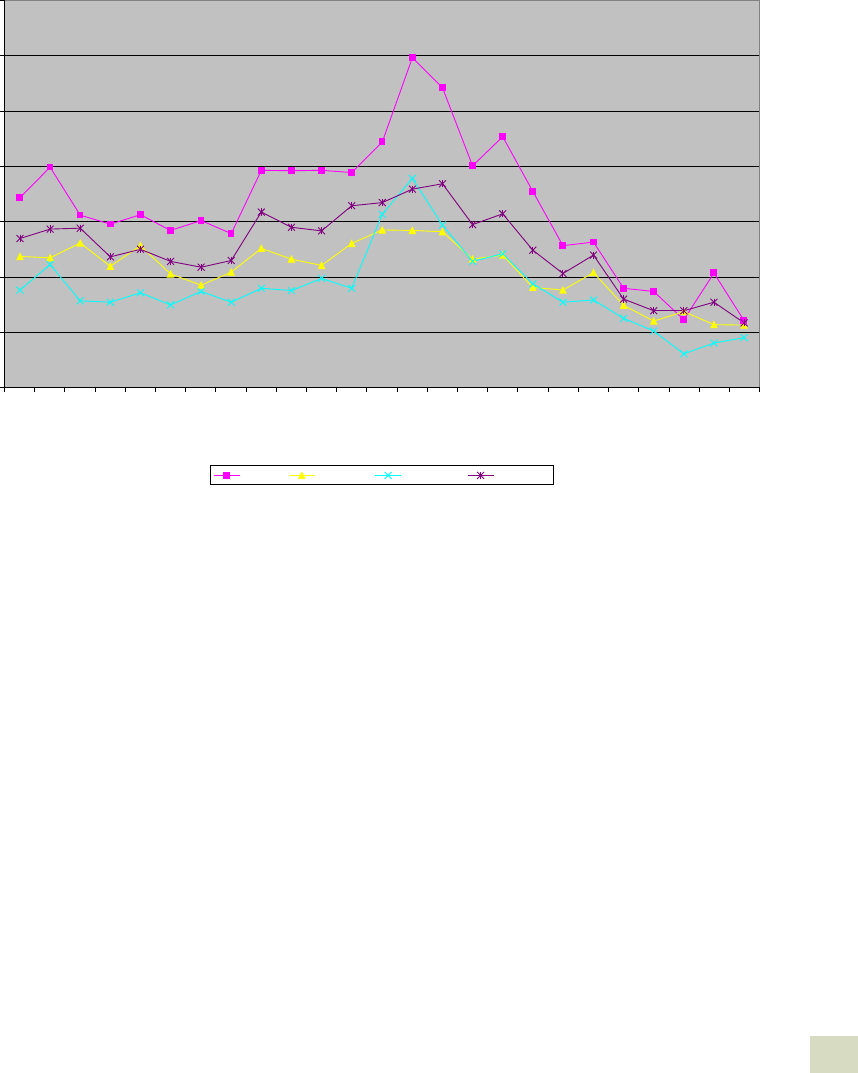
Understanding the “Whys” Behind Juvenile Crime Trends
27
percent between 1987 and 1993. Looking only at incidents of adult offending with no accompanying
juvenile offender, the rate for offenders perceived to be between ages 18 and 29 increased 53 percent
from the low in 1986 to a high in 1993, and the offending rate for persons over 30 declined slightly
during this period. If we limit juvenile offending to just those incidents with no adult involvement, we
see a similar pattern. Juvenile offending without adult involvement increased 153 percent from 1985
to 1993, while the increase for young adults was 69 percent. This suggests that during the late 1980s
and early 1990s, the increase in offending was large for both juveniles and young adults, but the
increase for crimes involving only juvenile offenders increased more than co-offending with adults.
Figure 2-7. Serious Violent Offending Rates for Juveniles and Young Adults with
and without Adult Co-offending, 1980–2004
From 1993 to 2004, the rate of serious violent offending by juveniles declined by 80 percent when
adult co-offending is included. The decline for persons 18 to 29 was 60 percent, and for persons over
30, offending rates dropped 54 percent. When adult co-offending is excluded from the juvenile trends,
the juvenile offending rates declined 84 percent, the young adult rates by 69 percent, and the rates for
persons 30 and older by 54 percent. The drop in juvenile offending was somewhat greater than the
decrease for other age-groups regardless of the treatment of adult co-offenders.
The differences in offending trends across age-groups are quite similar in the survey data and
arrest data. Increases in serious violent crimes by juveniles were greater than those observed for
adults, by a factor of more than two. The decreases in serious violent offending for juveniles were
greater than those for adults, but the differences across the age-groups in the rate of reduction are not
as great as the differences in the increases. Serious violent offending that involved only juveniles
increased more between 1985 and 1993 than juvenile co-offending with adults, while decreases in
juvenile-only offending and adult co-offending were very similar from 1993 to 2004. These
characteristics of the juvenile offending trends suggest that the processes driving the crime increase
0
2000
4000
6000
8000
10000
12000
14000
1980
1981
1982
1983
1984
1985
1986
1987
1988
1989
1990
1991
1992
1993
1994
1995
1996
1997
1998
1999
2000
2001
2002
2003
2004
Years
Rates per 100,000
<18 (1) 18-29 (1) All <18 (2) 18-29 (2)
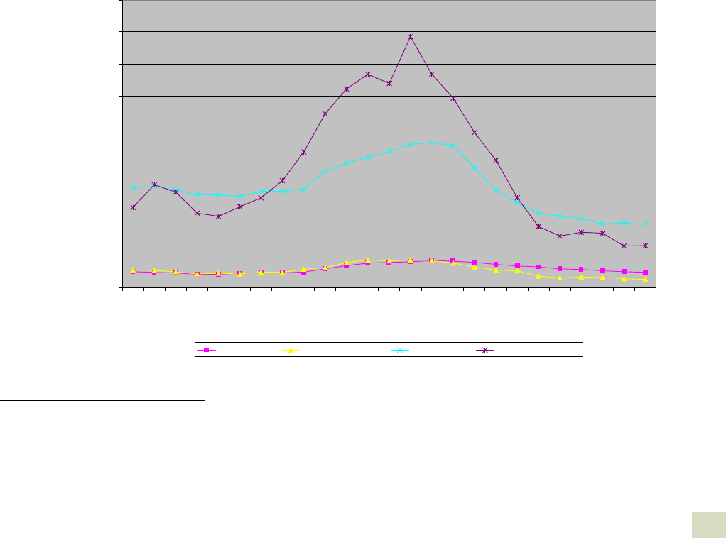
Understanding the “Whys” Behind Juvenile Crime Trends
28
were concentrated disproportionately among juveniles and that the factors driving the drop in crime
are operating in both the juvenile and young adult population.
Race of Offender. The common perception is that a disproportionate amount, if not the bulk, of the
increase and decrease in juvenile offending in the past 20 years was attributable to changes in the
behavior of black juveniles (Blumstein & Wallman, 2000). That perception is correct even though the
trend for Asian juveniles was more volatile, because black juveniles vastly outnumber Asian juveniles
in the population.
When we examine the contribution of each racial group to the increase in the number of juvenile
offenses during the period, it becomes clear that black juveniles account for the vast bulk of the
increase. The increase in the arrest of black juveniles for homicide accounts for 66 percent of the
increase in juvenile arrest rates for homicide compared to 32 percent for whites, less than 1 percent for
Native Americans, and 1 percent for Asians.5
Over the same periods, the homicide arrest rates for black juveniles increased 252 percent, from
22.3 per 100,000 in 1984 to 78.5 per 100,000 in 1993, while the rates for white juveniles increased only
94 percent (Figure 2-8). But the percentage increase in rates for Asians was even higher than for blacks
(470 percent from 1984 to the high point in the trend, 1996). The increase for Native Americans was
162 percent from 1984 to the high point in 1995. The homicide arrest rates for Native Americans and
Asians, however, are based on very small numbers and are very unstable.
Figure 2-8. Juvenile Arrest Rates for Homicide and Serious Violence by Race, 1980–2004
5
The proportion of the decline in juvenile offending attributable to a certain race was determined by subtracting the number of arrests
or offenses at the low point of the trend from the number at the high point to obtain the total decrease in juvenile offending. The same
subtraction was done for each race group. The remainder for each race group was divided by the total remainder to obtain the
proportion of the decline due to a specific race group. This procedure is used to determine the proportion of the drop due to specific
subgroups throughout the paper.
0.0
500.0
1000.0
1500.0
2000.0
2500.0
3000.0
3500.0
4000.0
4500.0
1980
1981
1982
1983
1984
1985
1986
1987
1988
1989
1990
1991
1992
1993
1994
1995
1996
1997
1998
1999
2000
2001
2002
2003
2004
Years
Juvenile arrests per 100,000 persons age 12to 17
White Violence White Homicide X 50 Black Violence Black Homicide X 50

Understanding the “Whys” Behind Juvenile Crime Trends
29
Black offenders also account for the bulk of the decrease in homicide by juveniles from 1993 to
2004. The homicide arrest rate for black juveniles decreased 83 percent, from 78.5 per 100,000 in 1993
to 13.2 per 100,000 in 2004. The arrest rate for whites declined from 8.6 per 100,000 to 2.6 or 69
percent. Percent changes tend to understate the decrease in black arrests because the base of the rate
in 1993 is so high. If we examine the change in the counts of homicide arrests over the period, we see
that black juveniles were responsible for 73 percent of the decline in homicide arrest rates from 1993
to 2004, compared with 26 percent for whites, less than 1 percent for Native Americans, and 1 percent
for Asians. Black juveniles, then, contributed substantially to both the increase and the decrease in
juvenile homicide offending.
In contrast with the juvenile arrest rate for murder, black juveniles did not account for the bulk of
the increase in the serious violence arrest rate between the mid-1980s and mid-1990s. The arrest rates
for serious violence increased 100 percent for whites from 1984 to 1994, the high point of the trend in
serious violence by white offenders. The rates for black juveniles increased 56 percent in the same
period, the rates for Native Americans by 112 percent, and the rates for Asians by 122 percent. Whites
account for 52 percent of the increase in arrests from 1984 to 1994, blacks for 45 percent, Native
Americans for 1 percent, and Asians for 2 percent. Whatever was driving the increase in serious
juvenile violence was operating for both whites and blacks, albeit more dramatically for black
juveniles.
Black juveniles do account for the bulk of the decrease in arrest rates for serious violence between
1993 and 2004. Arrest rates for black juveniles declined 56 percent over this period compared with 43
percent for whites. The decline in black juvenile arrests for serious violence accounts for 62 percent of
the overall decline in juvenile arrests for serious violence, compared with 37 percent for whites, less
than 1 percent for Native Americans, and 1 percent for Asians. This is very similar to what was
observed for homicide. In contrast to the rise in juvenile violent crime, the decline in serious juvenile
violence was driven more strongly by events or conditions in the black population than among white
juveniles.

Understanding the “Whys” Behind Juvenile Crime Trends
30
Figure 2-9. Juvenile Offending Rates for Serious Violence by Race with and without
Adult Co-offending, 1980–2004
The percent decline in the NCVS offending rates from 1993 to 2004 is very similar for both white
and black juveniles (Figure 2-9). Rates of offending for serious violence decreased about 70 percent for
both. This is not consistent with the serious violence arrest data, where the decreases are substantially
greater for blacks than for whites. The decreases in serious violent offending rates are more consistent
with the arrest trends when the change is assessed from 1993 to 1998. The rates of serious violent
offending decreased by 72 percent for blacks and by 40 percent for whites during that period. From
1998 to 2000, however, the rate of decrease for blacks slowed, while the rate of decrease for whites
continued apace.
The homicide arrest data show a similar trend, albeit less pronounced. The homicide arrest rate for
black juveniles decreased 58 percent between 1993 and 1998, while the white rate decreased 38
percent. When the period 1993 to 2000 is considered, declines in the white and black homicide arrest
rates are more similar: 64 percent for whites and 75 percent for blacks. This continued to 2004, when
the decrease from 1993 was 69 percent for whites and 83 percent for blacks. Beginning in 1998, there
was a substantial slowing of the decline in homicide arrest rates for blacks, but not for whites.
The same can be seen in arrest rates for serious violence. The decrease in these rates from 1993 to
1998 was 41 percent for blacks and 19 percent for whites. For the period 1993 to 2000, the drop was
50 percent for blacks and 30 for whites, and for the period 1993 to 2004, it was 56 percent for blacks
and 42 percent for whites. The declines in offending and arrest rates are much more similar across
races later in the period.
These trends in both the UCR and NCVS data suggest that whatever drove the increase in serious
violence during the late 1980s and early 1990s was not restricted to the black community; it also
substantially affected whites. The factors driving the decline in serious juvenile violence, however,
were more concentrated among black juveniles, except between 1998 and 2000, while the decline in
0
5000
10000
15000
20000
25000
30000
1980
1981
1982
1983
1984
1985
1986
1987
1988
1989
1990
1991
1992
1993
1994
1995
1996
1997
1998
1999
2000
2001
2002
2003
2004
Years
Rate per 100,000 persons 12-17
White any(x5) Black any
White all(X5)
Black all

Understanding the “Whys” Behind Juvenile Crime Trends
31
offending slowed among black juveniles and accelerated among white juveniles. After 2000, those
factors had substantially smaller effects for both groups.
Gender of the Offender. The common wisdom also has juvenile males accounting for the bulk of the
increase and decrease in juvenile violence since the mid-1980s. Again, this is true, but somewhat
overstated. Juvenile arrest rates for homicide increased more for males than they did for females from
1984 to 1993 (Figure 2-10). Over this period, the rate for males rose by 189 percent, from 12.4 per
100,000 to 35.8 per 100,000; in comparison, the females arrest rates for homicide rose 77 percent, from
1.3 to 2.2 per 100,000. However, the percentage increase in the juvenile arrest rates for serious
violence was greater for females from 1984 to 1993 than it was for males. The arrest rates for males
increased 71 percent, while those for females went up 117 percent. Although the increase in serious
violence by females was greater than that for males, male juveniles accounted for the overwhelming
majority of the increase in serious violence—83 percent of the increase in arrests for serious violence
and 96 percent of the increase in juvenile arrests for homicide.
Figure 2-10. Juvenile Arrest Rates for Homicide and Serious Violence by Gender, 1980–2004
The percentage drop in arrest rates for juvenile males between 1993 and 2004 was greater than
the drop for juvenile females. The juvenile male arrest rate for homicide fell 78.6 percent (from 35.8 per
100,000 to 7.7) and for serious violence, it declined by 50.6 percent (from 1,148 in 1993 to 567 in 2004).
The female arrest rate for homicide decreased from 2.2 to 0.8 or 64 percent. The serious violence rates
for females declined from 189 to 137, or only 28 percent. Males accounted for 96 percent of the
decrease in juvenile arrest rates for homicide and 96 percent of the decrease for serious violence.
The bulk of the increase and the decrease in arrests for serious violence is attributable to offenses
committed by males, so any search for causes must focus on the male juvenile population. The arrest
rate trends, however, increased more for females than males, and they did not decline as sharply as
0.0
200.0
400.0
600.0
800.0
1000.0
1200.0
1400.0
1980
1981
1982
1983
1984
1985
1986
1987
1988
1989
1990
1991
1992
1993
1994
1995
1996
1997
1998
1999
2000
2001
2002
2003
2004
Years
Arrest Rates per 100,000 Persons 12 to 17
Male Violence Male Homicide X10 Female Violence Female Homicide X 100
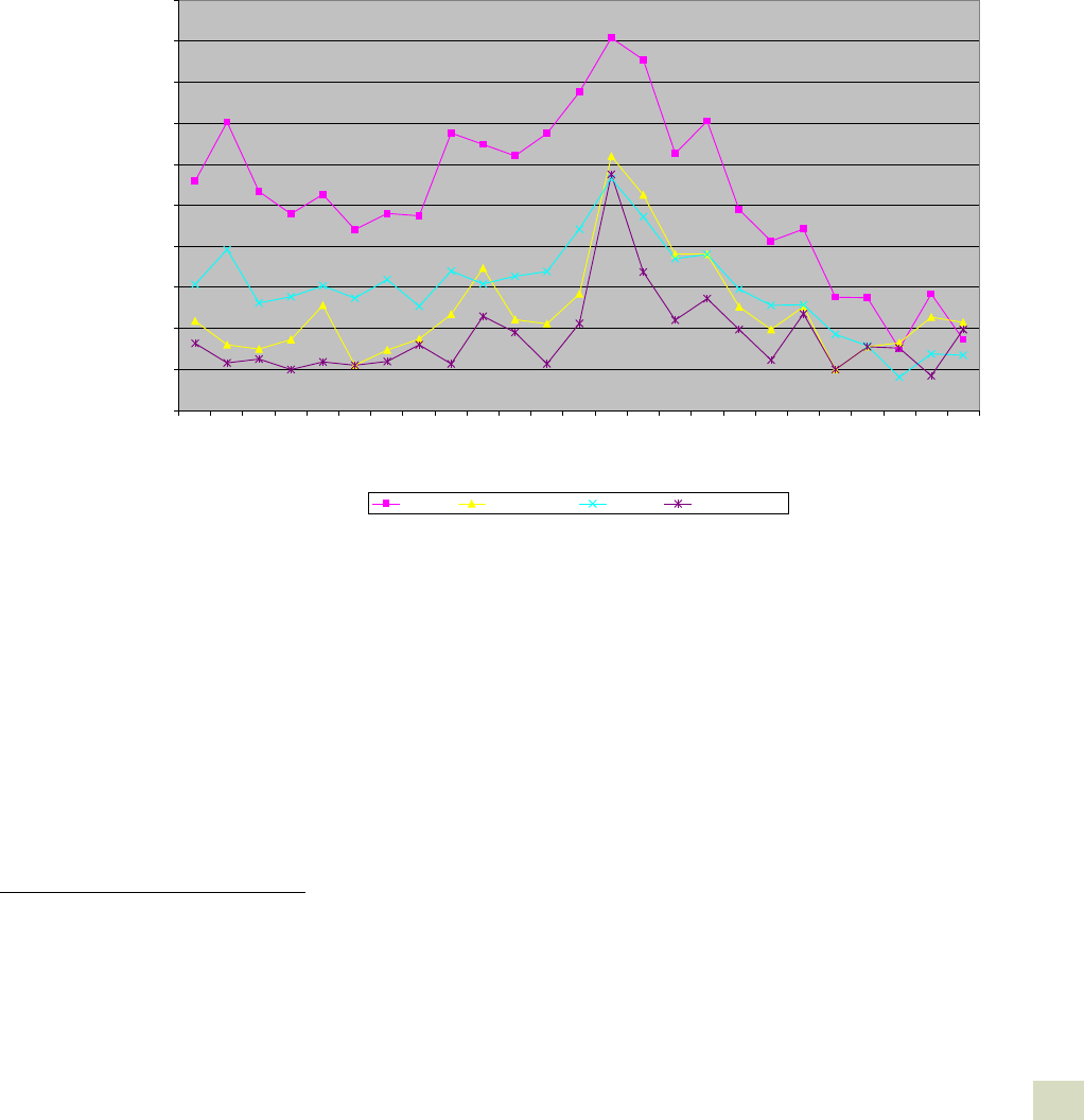
Understanding the “Whys” Behind Juvenile Crime Trends
32
the trends in violence by males. There appears to be a continuing secular trend in increasing arrests of
female juveniles for violence independent of the increase and decrease observed during this period.
The NCVS data tell a similar, if somewhat more complex, story. The serious violence offending rates
for both male and female juveniles increased between 1985 and 1992, but the increase for female
offending is greater than that for males (Figure 2-11). When adult co-offending is included in the rates,
the increase for males was 76 percent and the increase for females 158 percent. If adult co-offending is
excluded, the increases are 62 and 93, respectively.
6
So, as in the arrest data, the percentage increase
in serious violent offending is greater for females than males in the late 1980s and early 1990s.
Figure 2-11. Juvenile Serious Violent Offending Rates by Gender with and without
Adult Co-offending, 1980–2004
The decrease in offending rates was steeper for males than for females between 1993 and 2004.
7
Rates for females fell 65 percent in that period (66 percent if adult co-offending with juveniles is
included). The corresponding rates for males are 81 and 76 percent. As with the juvenile arrest rates,
the overwhelming majority of the drop is accounted for by the decrease in offending by males, as
males commit many more crimes than females. Males account for 86 percent of the decline in serious
violent offending (80 percent when adult co-offending is excluded).
The patterns of increases and decreases by gender are very consistent between the arrest records
and the victim survey results; both series show a sharper increase for females relative to male juveniles
from 1984 to 1992 and not as steep a decrease from 1993 to 2004. It is interesting to note that in the
6
1992 is used as the end point of the interval because there was a sharp increase in violent offending in the 1993 for females, but not for
males. Such a large jump in a single year is suspicious. It may be that the redesign of the survey has something to do with this increase
and our adjustments to the series did not take this into account. We thought that using 1992 would give a more accurate picture of the
differences in trends by gender.
7
The decrease was assessed at 1993 because this was the high point in the trend, and by using 1993 as the reference year, all of the
rates will be computed with data from the redesigned survey.
0
2000
4000
6000
8000
10000
12000
14000
16000
18000
20000
1980
1981
1982
1983
1984
1985
1986
1987
1988
1989
1990
1991
1992
1993
1994
1995
1996
1997
1998
1999
2000
2001
2002
2003
2004
Years
Rates per 100,000
male (1) female (1)(X5)
male (2) female (2) (X5)

Understanding the “Whys” Behind Juvenile Crime Trends
33
NCVS, the percentage decrease in serious violent offending by females during the 1990s is much more
similar to that for males than is the case in the arrest data. The percent decline for females in the arrest
data is roughly one-half that for males. This may occur because the survey data include a greater
proportion of more minor crimes than the police record data. The trend among very serious offenses
may be different than that for the lower end of serious crime. Alternatively, the trend in the arrest data
may be driven in part by changes in the police treatment of female offenders. They may have been
increasingly inclined to arrest female juvenile offenders, so that the trend reflects, in part, changes in
police practices and less so actual changes in criminal behavior. This is also consistent with the fact
that the percent decreases in homicide arrests were more similar for males and females than the
decline in arrest trends for serious violence. There is substantially more discretion to arrest and record
arrests for assault than for homicide, so that changes in police policy will affect the serious violence
trends more than those for homicide.
Trends in Other Attributes of Offending
The foregoing sections described changes in serious violent crime and in the demographic
characteristics of offenders. The NCVS (and to a lesser extent the UCR) provides an opportunity to
monitor changes in the social context of offending behavior. Specifically, we are able to assess
changes in the circumstances of the crime, such as number of offenders, whether the victim thought
the offenders were part of a gang, weapon presence, the relationship between victim and offender,
and the location of the crime. All of these attributes of crime events can suggest why they occurred.
Group Offending. Juveniles offend in groups to a much greater extent than adults do. In the period
1993 to 2004, the average annual serious violence offending rate for juveniles was 6,173 per 100,000
(Figure 2-12). Lone offending, where there was only one offender, accounted for 1,353 offenses per
100,000, and co-offending accounted for 4,827 offenses per 100,000. Overall, 78 percent of juvenile
offending is co-offending; more specifically 34 percent of juvenile offending is done with adult co-
offenders and 44 percent involves co-offending with other juveniles.

Understanding the “Whys” Behind Juvenile Crime Trends
34
Figure 2-12. Serious Violent Juvenile Offending Rates by Lone and Co-offending Status, 1993–2004
Over the period 1993 to 2004, co-offending with other juveniles declined more than co-offending
with adults and lone offending. Lone offending declined 76 percent, from 2,357 per 100,000 in 1993 to
1,240 per 100,000 in 2002. The adult co-offending rate declined 55 percent, from 2,809 per 100,000 in
1994 to 1,240 per 100,000 in 2002. The juvenile co-offending rate declined 90 percent, from 6,746 per
100,000 in 1993 to 661 per 100,000 in 2002.
For some reason, lone offending declined more than co-offending with adults, and co-offending
with juveniles declined the most. It may be that by reducing juveniles’ fear of violent victimization, the
decline in crime itself made “affiliating” with loose groups or gangs for self-protection less necessary.
Less affiliation would, in turn, accelerate the decline in victimizations by groups of juveniles.
Throughout the period 1993 to 2004, lone offending was a much higher proportion of the
offending rate for white juveniles than for black juveniles (Figure 2-13). Thirty-three percent of the
white juvenile offending rate for serious violence involved lone offending, while 36 percent involved
co-offending with adults and 31 percent involved co-offending with juveniles. In contrast, among
black juveniles, only 21 percent of serious violent offending was lone offending, 40 percent was co-
offending with adults, and 39 percent was juvenile co-offending. Co-offending is somewhat more
prevalent for black juvenile offenders than white.
0
2000
4000
6000
8000
10000
12000
14000
1993 1994 1995 1996 1997 1998 1999 2000 2001 2002 2003 2004
Years
Rates per 100,000
Lone Offending Adult Co-offending Juvenile Co-offending

Understanding the “Whys” Behind Juvenile Crime Trends
35
0.0
5000.0
10000.0
15000.0
20000.0
25000.0
30000.0
35000.0
1993 1994 1995 1996 1997 1998 1999 2000 2001 2002 2003 2004
Years
Rate per 100,000 Persons
White Lone Offending Rate White Co-offending Rate Black Lone Offending Rate Black Co-offending Rate
Figure 2-13. Offending Rates for Serious Violence by Offender Race and Lone and
Co-offending Status, 1993–2004
During the period 1993 to 2004, there was a large racial difference in co-offending status. Co-
offending with other juveniles declined by 92 percent for blacks and only 79 percent for whites. Lone
offending dropped in slightly greater or similar proportion for blacks than whites—69 percent versus
76 percent. Co-offending with adults also declined slightly more or similarly for black than for white
juveniles—83 and 78 percent, respectively. If the decline in overall juvenile co-offending was due to a
decline in the need to “affiliate” for safety or something else, that effect was stronger for black
offenders than for white.
These differences across race were more pronounced during the shorter period 1993 to 1998.
During those years, the percentage decline in lone offending rates was essentially the same for white
and black juveniles—43 percent. Decreases in the adult co-offending rate were greater for black
juveniles (63 percent) than white (50 percent). The big differences across races, however, occurred in
juvenile co-offending, where the decrease for black juveniles was 90 percent and that for whites only
29 percent.
Whatever the disincentives to group offending over the 1990s, they were greatest for juvenile co-
offending and they occurred in the black population earlier than they did among white juveniles.
Gang Involvement. In an attempt to understand the decline in co-offending, we examined a question
on the NCVS that asked the victim if he or she thought that the offenders were part of a gang. No
follow-up questions were asked to determine the basis of the inference, so it must be treated
cautiously at face value. The proportion of juvenile offending that victims perceived as involving gang
members declined from 24 percent in 1993 to 11 percent in 2000 (Figure 2-14). When adult co-
offending is included in the rates, the decline in perceived gang involvement is somewhat greater,
from 31 percent in 1993 to 12 percent in 2000. This is consistent with the decline in co-offending and

Understanding the “Whys” Behind Juvenile Crime Trends
36
suggests that reductions in perceived gang activity may account for some of the decline in juvenile
involvement in serious violent offending. The proportion of serious offending identified as involving
gangs began to rise after 2000, reaching 21 percent in 2004 for violent offending including adult co-
offending and 22 percent when adult co-offending is excluded.
When we examine the rates of serious violent juvenile offending, the patterns are similar. The rate
perceived to involve gangs decreased 70 percent from 1993 to 1998, from 3,728 per 100,000 to 1,119
per 100,000. When adult co-offending is excluded the rates decreased 77 percent, from 1,820 per
100,000 to 407 per 100,000. In contrast, the rates of serious juvenile offending without gang
involvement decreased 51 percent, from 8,209 per 100,000 in 1993 to 4,012 per 100,000 in 1998. The
decline in non-gang violence increased to 53 percent when adult co-offending was excluded. The
rates of decline for juvenile violence with and without gang involvement became more similar after
2000. The percent decrease in serious juvenile violence involving gangs from 1993 to 2000 was 88
percent, but the decrease from 1993 to 2002 only increased slightly to 91 percent. The percent
decrease in serious juvenile violence not involving gangs from 1993 to 2000 was 61 percent, and this
increased to 74 percent over the period 1993 to 2002. When adult co-offending is removed, the
decrease in serious juvenile offending with gang involvement decreased by 84 percent from 1993 to
2000 and by 94 percent from 1993 to 2002. In comparison, offending without gang involvement
decreased by 61 percent from 1993 to 2000, and 80 percent from 1993 to 2002.
Figure 2-14. Serious Violent Offending Rates with and without Adult Co-offending
by Gang Involvement, 1993–2004
0.0
1000.0
2000.0
3000.0
4000.0
5000.0
6000.0
7000.0
8000.
0
9000.0
1993 1994 1995 1996 1997 1998 1999 2000 2001 2002 2003 2004
Year
Rate per 100,000
Violence wo Gangs Any<18 Violence wo Gangs All<18
Violence with Gangs All<18 X 2
Violence with Gangs Any<18 X 2
Victim–offender Relationship. There was considerable variation in the victim–offender relationship
during the drop in juvenile offending. The proportion of juvenile offending in which the victim knew
the offender rose gradually over the decade from 28 percent in 1993 to 43 percent in 1998, only to fall
again, reaching 31 percent in 2000 before rising to 47 or 48 percent in 2004. When adult co-offending
is included, the trends are very much the same, going from 38 percent knowing the offender in 1993

Understanding the “Whys” Behind Juvenile Crime Trends
37
to 59 percent in 1998, dropping to 37 percent in 2000 and rising to 48 percent in 2004. The proportion
of offenders known to the victim increased from 1993 to 1998 because the proportion of violence
committed by strangers fell over the period. This trend of reductions in stranger-to-stranger violence
slowed from 1998 to 2000, only to reoccur from 2000 to 2004.
The story is similar when we look at the change in serious violent offending rates by victim–
offender relationship (Figure 2-15). From 1993 to 1998, the rate of serious violent juvenile offending
involving strangers declined 66 percent (73 percent when adult co-offending is excluded; Figure 2-16),
while the rate for offending against known victims fell 34 percent (36 with adult co-offenders
excluded). By 2002, the declines in violent offending between strangers and non-strangers became
much more similar. From 1993 to 2002, violent juvenile offending among strangers declined 85
percent (91 percent with adult co-offenders excluded), and offending involving non-strangers fell 72
percent (80 percent without adult co-offending).
Figure 2-15. Percent Known Victims in Serious Violent Juvenile Offending with and without
Adult Co-offending, 1993–2004
0.0
10.0
20.0
30.0
40.0
50.0
60.0
70.0
1993 1994 1995 1996 1997 1998 1999 2000 2001 2002 2003 2004
Years
Percent of Offending
Any<18 All<18

Understanding the “Whys” Behind Juvenile Crime Trends
38
Figure 2-16. Serious Violent Offending with and without Adult Co-offending by
Victim–Offender Relationship, 1993–2004
0
1000
2000
3000
4000
5000
6000
7000
8000
9000
1 2 3 4 5 6 7 8 9 10 11 12
Years
Offending Rates per 100,000
Known Offender Any<18 Known Offender All<18 Unknown Offender Any<18
Unknown Offender All<18
Figure 2-17. Proportion of Juvenile Homicide Offenses by Victim–Offender Relationship, 1976–2004
0%
10%
20%
30%
40%
50%
60%
70%
1976
1977
1978
1979
1980
1981
1982
1983
1984
1985
1986
1987
1988
1989
1990
1991
1992
1993
1994
1995
1996
1997
1998
1999
2000
2001
2002
2003
2004
Years
Percent
Relative Acquaintance Stranger
The homicide data show the same decrease in stranger-to-stranger offending throughout the
1990s (Figure 2-17). In 1993, almost 38 percent of homicides with offender information involved
strangers, and this proportion declined to 30 percent in 1999.
8
During the same period, homicides
8
The large category of homicides by acquaintance showed no pronounced pattern in the period.

Understanding the “Whys” Behind Juvenile Crime Trends
39
among intimates increased from 7 percent to 13 percent. This trend reversed itself in 2000, when the
proportion of homicides by strangers rose to 40 percent and remained between 36 and 39 percent
through 2004. The proportion of homicides involving relatives, about 8 percent throughout the 1990s,
rose to 13 percent in 1998, and stayed at approximately that level through 2004.
The drop in juvenile offending from 1993 to 2004 was characterized by a greater decrease in
stranger-to-stranger crime than violence among persons known to the victim. This may have occurred
because the opportunity for violence among strangers decreased, as where there was reduced contact
among strangers. It also may be the case that the social organization of contact among strangers
became safer than it was previously. The routinization of the drug trade, for example, would allow
strangers to interact in drug transactions, but more safely because dealers were not fighting over turf.
The absence of drug violence in public places would make interaction in these places
(disproportionately among strangers) generally more secure.
Location. Central cities (especially large central ones) figure prominently in discussions of the rise and
fall in violence, because violence is believed to be concentrated in these large urban centers. The 20
largest cities, for example, account for about 80 percent of the homicides (Blumstein and Wallman,
2000). The central place of these urban centers in the decrease in juvenile offending may be an artifact
of the UCR data or it may be more the case for homicide than it is for violent offending more generally.
The UCR overrepresents larger places, and the arrest data are not adjusted to take account of the
substantial amount of missing data in smaller jurisdictions (Maltz, 1999). As a result, the contribution
of large, central cities to the crime rates could be overestimated with the arrest data. Moreover,
homicide may be highly clustered in larger places, but other juvenile violent offending may not be.
The NCVS trends in serious juvenile offending indicate that the decreases in serious violent
offending by juveniles were about the same for central cities of Standard Metropolitan Statistical Areas
(SMSA), suburban areas, and rural areas (Figure 2-18). When adult co-offending is included in the
juvenile offending rates, the rate of juvenile offending in central cities decreased by 82 percent from
1993 to 2004, compared with a 79 percent decrease in the suburbs and a 76 percent decrease in more
rural areas. When adult co-offending is excluded, the percent decrease in offending rates in central
cities from 1993 to 2000 was 78 percent, with suburbs experiencing the same percentage decrease
and more rural places seeing a decrease of 66 percent.
Serious violent juvenile crime trends are not consistent with the “routinization of the drug trade”
explanation of the crime drop, which emphasized the changes in our largest cities. Central cities
accounted for 42 percent of the total decrease in serious violent offending by juveniles (40 percent
when adult co-offending is excluded), while suburban and rural places accounted for 58 percent (60
percent when adult co-offending is omitted). Although central cities account for a substantial portion
of the drop in serious violent offending by juveniles, the bulk of the decrease occurred elsewhere.
This suggests that any explanation or set of explanations for the crime drop cannot be restricted to
what has occurred in these large urban areas. This also gives greater credibility to the arrest rates
flowing from the UCR data.
This conclusion must be tempered by acknowledging the bluntness of the central city designation
in the NCVS. There, the term “central cities” refers to central cities of SMSA, and includes cities of
50,000 or more. This may be much too inclusive to distinguish what is happening in very large cities of
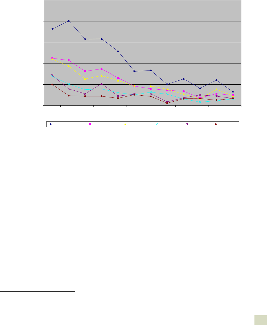
Understanding the “Whys” Behind Juvenile Crime Trends
40
250,000 or more residents.
9
Nevertheless, this does not change the fact that a great deal of the drop in
juvenile offending occurred outside of central cities, even when these areas are defined liberally.
Figure 2-18. Juvenile Serious Violent Offending Rates by Location with and without
Adult Co-offending, 1993–2004
0
5000
10000
15000
20000
25000
1 2 3 4 5 6 7 8 9 10 11 12
Years
Rates per 100,000 Persons
Central cities any<18 Central city all<18 Suburb any<18 Suburb all <18 Rural any<18 Rural all<18
Firearms. The diffusion of firearms from the drug industry to the wider community figures prominently
in some explanations of the increase and decrease in homicide, and by extension serious violence
(Blumstein & Wallman, 2000). The NCVS and the SHR data include information on whether a firearm
was used and whether the victim believed the offender was a juvenile. When adult co-offending is
included in the NCVS rates, there is a drop in the proportion of serious juvenile violent victimizations
involving a firearm, from 25 percent in 1993 to about 12 percent in 2002 (Figure 2-19). When adult co-
offending is excluded, there still is a large decrease in the use of firearms, from 22 percent in 1994 to 7
percent in 2002.
9
The NCVS includes data on city size that could be used to identify very large central cities. Unfortunately, during the period 1993 to
2000, the census updated its geographical information so that cities may not be consistently classified during that period.

Understanding the “Whys” Behind Juvenile Crime Trends
41
Figure 2-19. Percent of Serious Violent Juvenile Offending Involving Firearms with and without
Adult Co-offending, 1993–2004
0.0
5.0
10.0
15.0
20.0
25.
0
30.0
1993 1994 1995 1996 1997 1998 1999 2000 2001 2002 2003 2004
Years
Percent of Offending
any<18 all<18
The homicide data on juvenile offenders shows a similar decrease in the use of firearms (Figure 2-
20). In 1994, 81 percent of homicides known to have been committed by a juvenile involved a firearm,
and by 1999, only 62 percent did so. By 2003, this percentage increased to 69 percent, and then
dropped again to 64 percent the following year.
The juvenile arrest rates for possession of a weapon provide additional information on the
availability of weapons. The arrest rates of juveniles for weapons possession also declined about 48
percent during the period, from 303 per 100,000 in 1993 to 140 per 100,000 in 2002. All of these data
suggest that the carrying of weapons by juveniles and their use in serious violent offending decreased
substantially from 1993 to 2002. This drop occurs not only for homicides but also for lesser forms of
serious violence by juveniles.

Understanding the “Whys” Behind Juvenile Crime Trends
42
Figure 2-20. Juvenile Arrest Rate for Weapons Offenses and Ratio of Firearm to Non-firearm Homicides
by Juveniles, 1980–2004
0.0
50.0
100.0
150.0
200.0
250.0
300.
0
350.0
1980
1981
1982
1983
1984
1985
1986
1987
1988
1989
1990
1991
1992
1993
1994
1995
1996
1997
1998
1999
2000
2001
2002
2003
2004
Years
Rates
Weapons Offenses Ratio of Firearm to Non-firearm Homicides X 50
Trends in Drug Arrests
Drug offending has been linked to movements in the violent crime rate as a precipitant and as a
deterrent (Figure 2-21). Some argue that increases in the sale and use of drugs precipitated the
contests over drug markets which lead to violence and the use of firearms. These firearms diffused into
communities that hosted drug markets, resulting in a proliferation of gun violence there. The drop in
crime occurred as drug markets became more organized and the need for violence decreased
(Blumstein & Wallman, 2000). Pressure from drug dealers and the police reduced the availability and
necessity of carrying and using firearms to resolve disputes in these communities. The result was a
drop in juvenile violence in these areas, as drug distribution organizations disproportionally recruit
juveniles for street-level activities because they face weaker penalties than adults.
Alternative explanations would have drug enforcement as a means of deterring violence. Unlike
most enforcement activity, drug arrests are almost purely at the discretion of the police. Usually there
is no complainant, so the police must be proactive in finding drug offenders. They choose when,
where, and how often to look for drug activity and, as a result, drug enforcement activity affords the
police an opportunity to apply coercion when and where they see fit. Removing drug offenders can
reduce other forms of crime, including violent crime through incapacitation (Cohen & Canela-Cacho,
1994; Kuziemko & Levitt, 2001).
If the latter theory accounts for some of the drop in juvenile violent offending, we would expect to see
a negative relationship between drug offending and violent juvenile offending. As drug arrests
increase, the level of juvenile violence should decrease. It is not clear what the pattern between drug
offending and violent offending should be if it is the routinization of the drug trade that accounts for
the drop in juvenile violent offending. If the stability of the drug markets means that there are fewer
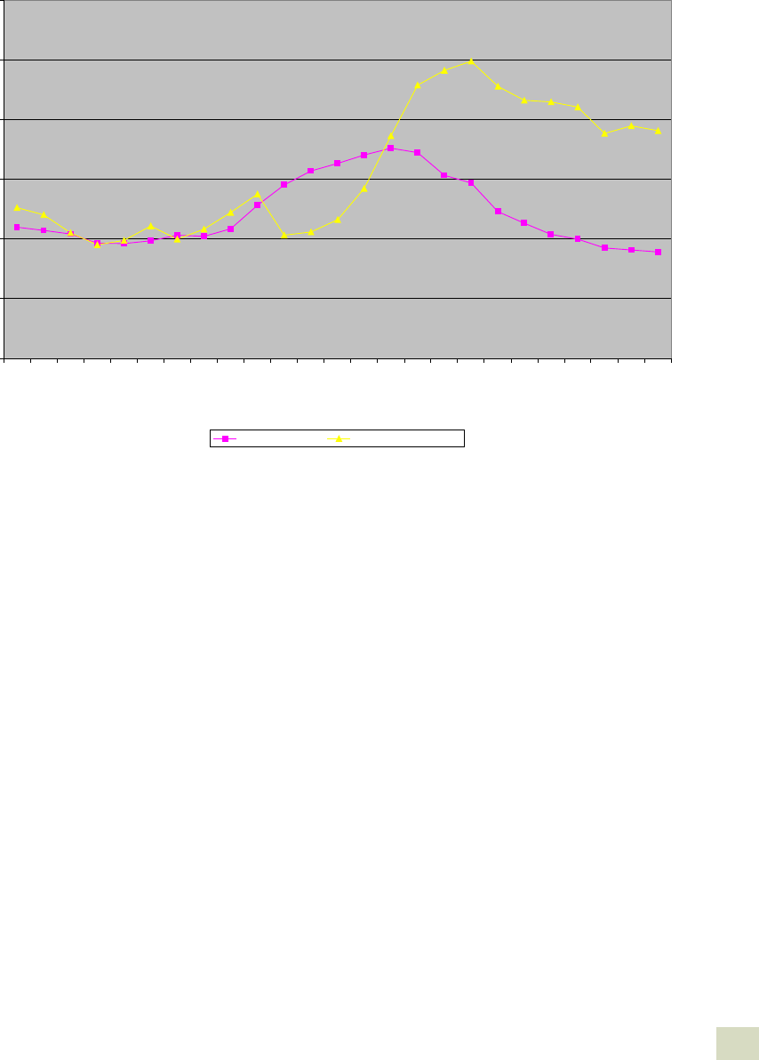
Understanding the “Whys” Behind Juvenile Crime Trends
43
traffickers and fewer consumers, then we should see a positive relationship between violence and
drug arrests. As the drug markets contract, drug arrests decrease and the level of violence decreases.
This need not be the case, however, as the volume of trafficking and consumption may have stayed
the same, while the violence attendant to disorderly markets may have decreased. This would result in
no relationship between drug arrest and violent arrests.
Figure 2-21. Juvenile Arrest Rates for Serious Violence and Drug Offenses, 1980–2004
0.0
200.0
400.0
600.0
800.0
1000.0
1200.0
Years
1980
1981
1982
1983
1984
1985
1986
1987
1988
1989
1990
1991
1992
1993
1994
1995
1996
1997
1998
1999
2000
2001
2002
2003
Year
Arrest Rates per 100,000 Persons 12 to 17
Serious Violence Drug abuse violations
There is no strong relationship between the trends in juvenile violence and the arrests of juveniles
for drug offenses over the entire period 1980 to 2004. If the trend is broken into three distinct periods,
however, we can see a relatively strong positive relationship between juvenile arrests for drugs and
juvenile arrests for violence. From 1980 to 1989, both type of arrests increased. From 1990 to 1995,
there also is a strong positive relationship between drug and violence arrests—as drug arrests
increase, so do rates of arrest for violence. Again from 1995 to 2000, there is a positive relationship
between the two trends, but in this period the trends are both decreasing. This positive relationship is
not consistent with the incapacitation or the drug substitution arguments that link drug offending and
violent offending. But it is consistent with the theories that link the routinization of drug markets with
drops in violence. As the violence attendant to an unregulated drug markets declines, so too do
arrests for drug offenses.
The relationship between drugs and violent offending is different for blacks and whites in the late
1990s (Figure 2-22). From 1994 to 2004, for white juveniles, increases in drug arrests were associated
with decreases in arrests for serious violence. This can be seen more easily in Figure 2-23, where
positive changes in the drug arrest rate are often associated with smaller positive changes in serious
violence or even negative changes in serious violence for whites, especially in this period. For black
juveniles, the opposite was the case; decreases in drug arrests were associated with decreases in
violence during that period (Figure 2-24). These trends suggest that there may be an incapacitation or
deterrence effect of drug offending for white juveniles but not for black juveniles. For black juveniles,

Understanding the “Whys” Behind Juvenile Crime Trends
44
the routinization of the drug trade arguments seems more consistent with the trends. If the decreases
in drug arrests are evidence of the routinization of the drug trade in black communities, then this
seems to be related to decreases in juvenile violence.
Figure 2-22. Juvenile Arrests for Serious Violence and Drug Offenses by Race, 1980–2004
0.0
500.0
1000.0
1500.0
2000.0
2500.0
1980
1981
1982
1983
1984
1985
1986
1987
1988
1989
1990
1991
1992
1993
1994
1995
1996
1997
1998
1999
2000
2001
2002
2003
2004
Year
Arrest Rates per 100,000 Persons 12 to 17
White Serious Violence White Drug Offenses Black Serious Violence
Black Drug Offenses
Figure 2-23. Change in White Juvenile Arrest Rates for Serious Violence and Drug Offenses, 1981–2004
-150.0
-100.0
-50.0
0.0
50.0
100.0
150.0
200.0
250.0
1981
Drug offense Arrest Rate
Serious Violence Arrest Rate
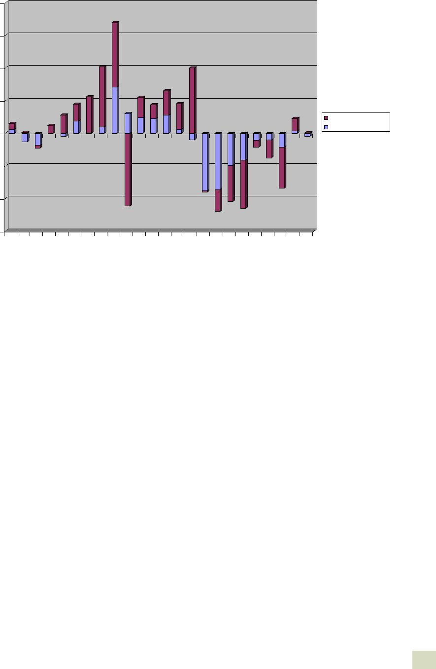
Understanding the “Whys” Behind Juvenile Crime Trends
45
Figure 2-24. Changes in Black Juvenile Arrests for Serious Violence and Drug Offenses, 1981–2004
-600.0
-400.0
-200.0
0.0
200.0
400.0
600.0
800.0
1981 1983 1985 1987 1989 1991 1993 1995 1997 1999 2001 2003
Drug Offense Arrests
Serious Violence
These trend comparisons are too simple to tell us much about the relationship between drug
offending and violent offending among juveniles. More sophisticated modeling is in order at both the
national and subnational levels. These comparisons do suggest, however, that the relationships
between drug offending and violent juvenile offending will differ for blacks and whites and across
different time periods. Subsequent investigation and modeling of this relationship should take this
into account.
Trends in Juvenile Offenders in Adult Prisons
Punishment, usually in the form of incarceration, is one of the most popular responses to
offending. The increases in crime in the late 1980s prompted demands to “get tough” on juvenile
offenders. One of the most controversial methods of increasing punishment for violent offending is to
transfer juvenile offenders to adult court where they are widely expected to receive harsher sentences
that must be served in adult correctional facilities. Evidence is mixed on whether the sentences in
adult court actually result in longer incarceration time.
In any event, to the extent that sentencing juveniles to adult facilities deters crime or incapacitates
offenders, we would expect a negative relationship between trends in the number of juveniles
sentenced to adult facilities and serious violent offending by juveniles. This, however, does not seem
to be the case. Increases in admissions of juveniles to state adult correctional facilities kept pace with
increases in the crime rate from 1986 to 1994, after which decreases in admissions were associated
with decreases in the violent juvenile offending rate (Figure 2-25). The same general relationship is
observed when the stock population of juveniles in adult facilities is used (Figure 2-26). Increases in
the stock of juveniles in adult facilities is associated with increases in the rate of serious violent
offending by juveniles in the late 1980s and 1990s, and decreases in the stock incarceration rate are

Understanding the “Whys” Behind Juvenile Crime Trends
46
associated with decreases in juvenile violent offending in the mid- to late 1990s. While these simple
comparisons of trends are no substitute for more complex modeling with lags and other refinements,
they are not consistent with sentences to adult institutions having a deterrent or incapacitation effect
on serious violent crime by juveniles.
Figure 2-25. Juvenile Arrest Rates for Serious Violence and Juvenile Admissions to Adult Prisons,
1985–2002
0.0
100.0
200.0
300.0
400.0
500.
0
600.0
700.0
800.0
1985 1986 1987 1988 1989 1990 1991 1992 1993 1994 1995 1996 1997 1998 1999 2000 2001 2002
Year
Rates per 100,000
Arrests per 100000 Juvenile Admissions per 1000000
Figure 2-26. Juvenile Stock Imprisonment Rates and Serious Juvenile Violent Arrest Rates, 1985–2002
0.0
100.0
200.0
300.0
400.0
500.0
600.0
700.0
800.0
1985 1986 1987 1988 1989 1990 1991 1992 1993 1994 1995 1996 1997 1998 1999 2000 2001 2002
Years
Rates per 100,000
Arrest Rates Per 100000
Prison Stock Rates Per 1000000

Understanding the “Whys” Behind Juvenile Crime Trends
47
Conclusion
The trends presented in the foregoing sections provide a starting point for understanding the drop
in juvenile offending during the past decade. The disaggregated trends in juvenile offending identify
the populations that experienced the greatest (or the least) change in offending and they describe the
changes in the characteristics of offending. This information can be used to guide the more complex
analyses necessary to determine causes of the drop in crime. Theories that can account for the
distribution of offending across population groups or the observed change in the characteristics of
offending will be given higher priority in subsequent testing.
The trends indicate that increases and decreases in offending behavior were more pronounced for
juveniles than they were for adults. Juvenile rates of serious violent offending increased more than
adult rates in the late 1980s and decreased more in the mid-1990s. The change in offending for young
adults (i.e., ages 18–20) was similar to that for juveniles and much higher than that for even slightly
older adults. Whatever is driving the increase and decrease in juvenile offending is peculiar to
juveniles and young adults during this period. The effects on older offenders are not nearly as strong.
The increase in serious violent offending in the late 1980s was not concentrated among black
juveniles, except for homicide. The decrease in serious violent offending in the 1990s, however, was
more concentrated among black juveniles. Moreover, the decrease in black juvenile offending
accounted for the bulk of the decrease in juvenile offending during the period. Again, whatever is
driving the decrease in juvenile offending, it is occurring with blacks more than with whites, but
occurring with whites as well.
The trends in juvenile offending by gender were similar in the police and survey statistics. Both
series showed a sharper percentage rise in serious violence for females in the late 1980s and 1990s
and a more modest drop in offending for females thereafter. These trends would be consistent with an
explanation that attributed the increase in female offending to a combination of processes that were
period-specific and others that were more long term. The rise of the drug trade and the diffusion of
violence from it, for example, would be a period-specific process. Changes in the status of women
would be a longer term process affecting the participation of women in crime and the probability of
arrest. These processes moved in the same direction in the late 1980s, causing sharper increases in
female violent offending. As the period-specific processes reversed themselves and the longer term
processes continued, the declines in serious violence among females were less pronounced than they
were for men who were affected by the period-specific processes only. While these differences in the
trends are interesting, the overwhelming majority of both the increase and decrease in juvenile
offending is attributable to male juvenile offending.
There were a number of suggestive changes in the social organization of offending between 1993
and 2004. First, the decline in group offending by juveniles was greater than the decline in lone
offending and greater for co-offending with other juveniles than for co-offending with adults. The
decline in juvenile co-offending was much greater for black juveniles than for white juveniles in the
period 1993 to 1998, but the declines across the two races in co-offending became more similar after
1998. These differences in lone and co-offending over time and across races need to be explored
further. Certainly, fewer gangs or less need to affiliate for self-protection must be examined as reasons
for these patterns. A second and related change in the nature of juvenile offending has been the

Understanding the “Whys” Behind Juvenile Crime Trends
48
decrease in perceived gang offending. Victims of serious violent offending by juveniles were less likely
to perceive the offenders to be members of a gang in 2000 than they were in 1993.
Third, the proportion of serious juvenile violence involving strangers declined throughout the
1990s. This may mean that strangers interacted less over time, or that the nature of the interaction
became less risky, or that the public places where strangers interacted became safer. Whatever the
process, theories of the drop in juvenile crime must be able to account for this drop in stranger-to-
stranger violence by juvenile offenders.
Fourth, the use of firearms in serious violent offending decreased from 1993 to 2000. This was
observed both in the homicide data and the survey data.
All of these changes in the social organization of juvenile offending during the 1990s suggest
strongly that period effects were at work in the drop in juvenile offending. Early socialization that
would produce cohort effects may influence the motivation to commit crime, but it should not
produce these very specific changes in the social organization of offending. It will not affect the choice
to offend in groups or gangs, for example, or the decision to prey upon strangers or intimates. These
decisions are influenced by more contemporaneous factors. Group offending, for example, is
influenced by the availability of groups or gangs or the necessity to travel in groups for self-protection
in high-crime periods or areas. When these opportunities or exigencies pass, the social organization of
(and, perhaps, even the level of) offending changes. This is not to say that cohort effects are not
operating, but that, if they are operating, they are doing so in concert with period effects.
The trends in juvenile offending by location do not show that the drop occurred largely in larger
urban places. The decline in serious violent offending from the NCVS was similar for central cities and
for other places. The bluntness of the central city classification in the NCVS may contribute to the non-
distinctiveness of central city crime declines. More importantly, however, central cities accounted for
42 percent of the decrease in juvenile crime, but 58 percent of that decline occurred in other places.
Consequently, explanations for the drop in juvenile crime cannot rely exclusively on social processes
occurring in central cities. A great deal was going on elsewhere.
The trends in drug offending by juveniles do not follow the same patterns as other offenses.
Arrests for drug offending did not decline as much or as soon as arrests for other crimes. Arrests for
drug crimes are not strongly related to arrests of juveniles for serious violence. When these trends are
separated by race, drug arrests are negatively related with serious violent offending for whites and
positively associated with serious violent offending for blacks. As drug arrest rates increased during
the 1990s, the arrest rates for serious violence declined for white juveniles. In contrast, as drug arrest
rates declined for black juveniles, the arrest rates for serious violence declined as well.
This pattern of juvenile drug arrests and arrests for serious violence is broadly consistent with other
trends in the data as well as some of the processes identified by Blumstein and Wallman (2000). The
decline in serious violence occurred disproportionately among black juveniles. These declines in the
black juvenile offending rate were greater for co-offending and group offending than for offenses
involving a lone juvenile. There were also signs of decline in offenses involving weapons and involving
strangers. All of these trends are consistent with the general “drop in crime” arguments presented by
Blumstein and Wallman (2000) and their colleagues.

Understanding the “Whys” Behind Juvenile Crime Trends
49
Some trends suggest that different processes may be at work among white juveniles. Their
declines in offending are a substantial part of the drop in serious violent crime, yet the contours of that
decline are different. The relationship between juvenile drug and violence arrest rates are different for
whites and blacks. Declines in serious juvenile violence are smaller for whites than for blacks. Declines
in co-offending in the 1990s are less pronounced for whites than for blacks. The drop in white
offending continued during the later 1990s but slowed for blacks. These differences suggest that the
processes driving the decline in offending by white juveniles may be different from those driving the
decline among black juveniles. More attention should be given to developing and testing theories
that would account for the decline in offending by white juveniles.
The trends also suggest that it may be useful to think of the decline in juvenile crime in phases,
where one set of factors accounts for the decline in one period and another set in another period. The
period 1993 to 1998 appears to be unique in some ways. The decreases were greater for black than for
white juveniles; co-offending declined more sharply than lone offending for black youths; offenses
with and among strangers and crimes with firearms declined substantially; and homicide and robbery
declined more than aggravated assault and rape. After 1998, the declines were different. The drop in
crime was not as steep as in the earlier period. It occurred more among whites than previously;
declines were greater in aggravated assault and forcible rape than in robbery and homicide; the
proportion of violent crime involving gangs and firearms began to increase. These differences suggest
that the factors driving the decline in juvenile crime in the recent past may be quite different than
those operating in the initial phases of the decline.

Understanding the “Whys” Behind Juvenile Crime Trends
50
Chapter 3. Community Characteristics and Juvenile Crime
Trends
Overview
Chapter 2 described juvenile crime trends between 1993 and 2000 as they were measured at the
national level. Our first task in Chapters 3–5 is to account for those trends in terms of measurable
conditions and processes in communities, whose local trends combine to generate national trends.
Our second task is to assess the value of those measures in local-level models that planners can use to
inform juvenile justice policymakers about likely future juvenile crime trends and to analyze potential
effects of policy changes and events on juvenile crime levels.
This chapter is concerned with conditions and processes that we classified as “community-level,”
meaning they are either defined or most readily measurable in terms of some administrative or
geographic area such as a county, neighborhood, or police beat. The five primary categories we
examined are:
The proportion of the population in demographic categories that are at highest risk of
offending;
The extent and concentration of poverty in a community;
Family and household structure;
Social organization (i.e., the capacity of a community to maintain order through informal social
processes); and
The array of legitimate and illegitimate income-earning opportunities available to residents of
a community.
In subsequent chapters, we examine how developmental and cultural factors and changes in
public policy have affected recent trends in juvenile crime.
As discussed in Chapter 1, our intent is to meet a specific need in juvenile justice policy analysis
rather than to develop a complete scientific explanation of recent trends in juvenile crime.
Accordingly, our emphasis is on possible causes and correlates of juvenile crime that: (1) have been
linked theoretically and/or empirically to juvenile crime; (2) varied over time in a manner consistent
with juvenile crime between 1985 and 1998; and (3) can be measured with indicators that local
governments regularly collect so as to be useful as leading indicators of local juvenile crime trends.
In the remainder of the chapter, we review research on community characteristics and crime—
particularly research focusing on juvenile crime and/or recent trends in crime—and compare national
trends in these factors with those in juvenile crime during the 1980s and 1990s.
1
1
Although national trends may not be indicative of those among the highest risk places (or groups), Chapter 2’s examination of juvenile
crime trends showed that the national drop in juvenile violence was not limited to high-risk areas like central cities. Accordingly, we
believe it is useful to examine national trends in factors thought to be causally related to juvenile crime trends. Further, a number of the
studies discussed in this chapter, including our own study of trends in large counties (see below), explore these relationships for smaller
areas like counties, cities, and neighborhoods.

Understanding the “Whys” Behind Juvenile Crime Trends
51
As our review shows, there has been relatively little research examining the links between recent
trends in community characteristics and juvenile crime. Therefore, we supplemented this review with
our own study of community characteristics and violent juvenile crime in 134 of the nation’s largest
counties. The analysis, which is referenced throughout the chapter and reported in detail in Appendix
A, assesses how changes in various community characteristics were related to the change in violent
juvenile crime (as measured by arrests of juveniles for violence) during the 1990s. The analysis
complements our descriptive assessment of national trends by providing a more rigorous test of
whether and how structural factors affected juvenile crime at the local level in large jurisdictions that
had a substantial impact on national crime trends.
Part 1:
Community Characteristics and Juvenile Crime: Prior Research and Recent Trends
Size of the High-Risk Population
The Youth Population
Two well-documented facts in criminology are that (1) individuals are most likely to commit crimes
during adolescence and young adulthood, and (2) males commit more crimes than females (Huizinga
et al., 2003; Sampson & Laub, 1992). An obvious implication of this is that ebbs and flows in the size of
the adolescent and young adult population, and particularly the male population, should coincide
with ebbs and flows in aggregate crime counts and rates. Because the ratio of males to females in the
juvenile population is generally steady (see National Center for Health Statistics [NCHS], 2004), most of
the discussion below focuses on age and crime.
Most evidence affirms that the age structure of the population influences total crime rates (South
and Messner, 2000). But more importantly for our purposes, some have theorized that the size of the
young population affects crime rates among the young themselves—specifically, cohorts of young
people who account for a larger share of the total population are expected to offend at higher rates
because they are more difficult to control and face more competition for jobs and other economic
opportunities (Easterlin, 1978, 1987). This hypothesis, however, has received mixed support at best,
particularly with respect to juvenile violence (Lauritsen, 2003; O’Brien, 1989; O’Brien et al., 1999;
Savolainen, 2000; Steffensmeier et al., 1992). For example, two national time-series studies of the
1960–1995 period reached opposite conclusions. One found that youth cohort size was significantly
related to age-adjusted homicide rates (O’Brien et al., 1999), but the other found that it was not related
to age-adjusted rates of total violent crime (Savolainen, 2000).
From 1980 to 1990, the percentage of the population ages 12 to 17 declined from 10.3 percent to
8.1 percent, and the percentage of the population consisting of males in that age range dropped from
5.3 percent to 4.1 percent. From 1990 to 2000, these percentages rose from 8.1 percent to 8.6 percent
and from 4.1 percent to 4.4 percent, respectively. Consequently, changes in the relative size of the
youth cohort do not appear to explain the rise in juvenile violence during the 1980s or its fall during
the 1990s (National Center for Health Statistics, 2004; U.S. Census Bureau, resident population
estimates by age, sex, and race for the years 1970–1996). A similar argument was made by Blumstein
(2006).

Understanding the “Whys” Behind Juvenile Crime Trends
52
As reported in Appendix A, changes in the percentage of the population consisting of males ages
12 to 17 were positively and significantly associated with changes in the juvenile arrest rate for
violence during the 1990s after controlling for various measures of poverty, family disruption, social
disorganization, legitimate and illegitimate economic opportunities, and other factors. However, the
relative size of the youth population grew in these counties during the 1990s and appeared to
increase juvenile violence about 5 percent, thus working against the overall downward trend in
juvenile violence in these areas.
Donohue and Levitt (2001) provide an alternative but related explanation for the crime drop of the
1990s. They propose that the legalization of abortion through the Roe v. Wade decision in 1973
reduced the size of the cohort of juveniles with the highest risk for offending. According to this
theoretical approach, while the juvenile population was growing in the 1990s, the number of at-risk
juveniles actually was declining because of a reduction in the number of unwanted pregnancies. They
base their analysis on state-level data on aggregate abortions and crime rates. Those states with the
higher numbers of legalized abortions experienced the greatest crime drop even when they
controlled for variables such as unemployment and poverty. Additionally, states that legalized
abortion at earlier dates (five did so in 1970 before the Roe v. Wade decision) experienced a reduction
in crime before states that lagged behind in changing their abortion policies.
Abortion and the Youth Population
Donohue and Levitt’s (2001) theory generated both attention and criticism (see Abramsky,
2001;Cook and Laub, 2001). Smith and Simon (2001) tested the theory with cross-national data. They
examined the relationship between crime and abortion in several Western European countries with
characteristics similar to those of the United States (Austria, Canada, Denmark, the Netherlands,
Norway, and Sweden). They analyzed abortion law from the 1995 United Nations Publication Abortion
Policies: A Global Review, and they used data from the International Criminal Police Organization
(INTERPOL).
Overall, their findings yield somewhat mixed results and do not lend a great deal of support for
Donohue and Levitt’s assumption that reducing the number of unwanted pregnancies through
abortion reduces crime. Every country except the United States and Sweden experienced decreased
fertility rates after abortion was legalized. In regard to the violent crime rates, all the countries except
the Netherlands and Sweden reported a reduction in homicide 15 to 25 years after the legalization of
abortion. The rates for assault, however, told another story. Every country included in the study had
higher rates of assault 15 to 25 years after the legalization of abortion, and almost every country
experienced higher rates of violent theft during this time period (with the exception of Denmark and
Sweden). The countries included in this study did not experience the same dramatic crime drop that
the United States experienced, and only Canada and Sweden reported overall reductions in the rates
of all crime.
Smith and Simon (2001) suggest that, in addition to aggregate numbers of abortions, the
availability of contraception should be examined in analyzing the relationship between the reduction
of unwanted pregnancies and lower crime rates. Berk and colleagues (2003) studied the association
between homicides of 15- to 24-year-olds and the lagged effect of the legalization of abortion. They
found that there was an association, but other factors, such as the decline in crack cocaine use, should
also be more fully explored.

Understanding the “Whys” Behind Juvenile Crime Trends
53
Hay and Evans (2006) tested the underpinnings of Donohue and Levitt’s theory by examining the
relationship between unwanted pregnancies and subsequent juvenile crime. The data used in this
analysis were collected between 1964 and 1969, before the Roe v. Wade decision (the data also were
collected before abortion was legalized in California, Alaska, New York, Hawaii, and Washington in
1970). They hypothesized that unwanted pregnancies would result in higher levels of delinquency
during adolescence and early adulthood, and that the effects of unwanted or mistimed pregnancies
would vary based upon the gender of the child and the characteristics of the mother, such as age and
marital and socioeconomic status. They found moderate support for these hypotheses. Male juveniles
from “unwanted” or “mistimed” pregnancies were significantly more likely to be involved in
delinquency. This pattern held true for serious delinquency as well, but faded with age. Overall, the
results of this study suggest that while there is a positive effect of unwanted pregnancy on
delinquency, this effect would explain “no more than 1% of the variation in general or serious
delinquency,” and thus would explain very little of the crime drop that occurred in the 1990s.
Logan and colleagues (2007) also provide a review of the literature on the impact of unintended
pregnancies on the well-being of the child and family. They report that the research on the
consequences of “unwantedness” shows that it leads to poor mental and physical health outcomes for
the children that may last from infancy (e.g., lower birth weight very often) to adulthood (lower
educational outcomes). However, they note that very few studies have actually examined the
relationship between pregnancy intentions and actual behaviors, such as delinquency, in adolescence.
They pull from the research reported above (see Hay & Evans, 2006). This lends some support to
Donohue and Levitt’s theory, but clearly, more research is needed before any sound conclusions can
be reached.
Finally, perhaps the most straightforward critique of the abortion thesis is that provided by
Zimring (2007: 85–103) who, among other arguments, shows that the proportion of births involving
children at higher socioeconomic risk did not decline following Roe v. Wade as hypothesized by
Donohue and Levitt. To approximate births of higher-risk children, Zimring examined trends in the
proportion of births to black mothers, single mothers, and single mothers ages 15 to 19. None of these
proportions decreased following the legalization of abortion; on the contrary, the latter two continued
growing for a number of years. Most notably, the percentage of children born to single teenage
mothers grew from 3.3% in 1965 to 5.1% in 1970 and then continued growing to 7.1% by 1975
(Zimring, 2007: 94–95). Although it is possible that the legalization of abortion reduced the rate of
growth in births of high-risk children, it did not reduce these births below their pre-legalization levels.
This makes it more difficult to attribute the 1990s reduction in juvenile violence to the change in the
legal availability of abortion.
Regardless of how this debate is resolved, future changes in abortion policy, should they occur, will
have rather limited value for researchers and practitioners attempting to forecast short-term local
juvenile crime trends. Obviously, the effects of such policy changes on juvenile crime would not be
realized for more than a decade.
Youth Born to Young Mothers
Of course, not all adolescents are at equal risk of delinquency. Those growing up in areas with high
levels of poverty and family disruption, for example, are at greater risk. In subsequent sections, we
consider how changes in poverty and family structure have affected juvenile crime. Here, we consider

Understanding the “Whys” Behind Juvenile Crime Trends
54
another factor that may be used to refine the measurement of high-risk youth cohorts: maternal age at
childbirth.
2
A number of studies suggest that children born to younger mothers, and to teenagers in particular,
are at higher risk for later delinquency and crime (Farrington, 2000; Jaffee et al., 2001; Nagin &
Tremblay, 2001; Pogarsky et al., 2003). In part, this is because young mothers are more likely to be poor
and to have deficient parenting skills. Maternal age at childbirth also has been hypothesized to
influence juvenile behavior through biological mechanisms (Orlebeke, 2001). Young mothers have
higher levels of testosterone during gestation, which is hypothesized to make their children more
aggressive through its influence on nervous system development. Younger mothers also are more
likely to engage in behaviors such as smoking that may have adverse effects on their children’s
biosocial development (Rasanen et al., 1999). For all of these reasons, children born to younger
women are hypothesized to have higher levels of disruptive, “externalizing” behaviors (i.e., aggressive,
overactive, or oppositional behaviors) that are potential precursors to delinquency.
Support for an aggregate relationship between births to young mothers and juvenile crime was
provided by Orlebeke (2001), who computed the ratio of the number of births to teenage mothers
(defined as younger than 20 years of age) to the number of births to older mothers (defined as ages 30
to 35) during each year between 1970 and 1980. He then correlated this ratio with the juvenile
offending rate (using Uniform Crime Report [UCR] Index arrests of 17-year-olds as the measure of
juvenile offending between 1987 and 1997). The correlation between the two time series was high
(Pearson correlation=0.71 and Spearman correlation=0.77).
The birthrate of children born to teens between the ages of 15 and 19 dropped from 89.1 in 1960
to 68.3 in 1970 and 51.0 in 1985 (births per 1,000 females aged 15–19) (Child Trends, 2008).
Additionally, the trend in fertility rates in the United States has moved toward older mothers. This
trend likely had a number of causes, including greater numbers of women in the workforce, the
liberalization of abortion laws resulting from the U.S. Supreme Court’s Roe v. Wade decision in 1973
(Donohue & Levitt, 2001), and a trend toward a preference for smaller families. At any rate, it is a trend
that is plausibly linked to the crime drop of the 1990s. Its effects, however, have not been studied in a
rigorous manner or at the local level. Further, neither this trend nor the liberalization of abortion laws
in the 1970s can explain the increase in juvenile crime during the late 1980s.
Implications for Developing Leading Indicators of Juvenile Violence
Projections of the size of the juvenile population will likely be needed to estimate juvenile crime
trends within localities. Although the size of the juvenile population may not affect rates of juvenile
crime, it will affect counts of juvenile crime, and these counts are most essential for planning purposes.
Further, there are methodological reasons for focusing on counts when modeling relatively rare
events (i.e., violent juvenile crimes) for small areas like police districts or neighborhoods.
2
The size of the non-white youth population, particularly that of black males, also might be used to refine the measurement of high-risk
youth cohorts. However, the racial composition of an area tends to be highly correlated with other measures of disadvantage, such as
poverty and family disruption, which are discussed in subsequent sections. In empirical analyses, race effects often disappear when such
factors are taken into account (Sampson & Lauritsen, 1993). At any rate, recent changes in the black male population have not been
consistent with changes in juvenile crime. U.S. Census figures show that from 1980 to 1990, the share of the population consisting of
black males ages 12 to 17 dropped from 0.75 percent to 0.62 percent. From 1990 to 2000, this share rose from 0.62 percent to 0.65
percent.

Understanding the “Whys” Behind Juvenile Crime Trends
55
Small-area statistics based on records of the ages and addresses of mothers who give birth are
likely to be available and updated periodically from local health departments, based on the source
documents submitted to NCHS. Analyzing the relationship between these data and local juvenile
crime, lagged appropriately in a local forecasting model, could potentially improve our ability to
forecast local juvenile crime trends and yield new evidence about the hypothesized correlation
between maternal age at childbirth and delinquency. However, projections for small areas based on
birth records will be complicated by inward and outward migration of families.
Poverty
Criminologists long have theorized that adverse economic conditions, including poverty, foster
crime. Determining the causal effect of poverty on crime is complicated by the difficulty of
distinguishing poverty’s effects from those of other negative social conditions (e.g., family disruption,
racial segregation) with which it is often associated (Bjerk, 2007; Land et al., 1990; see also reviews in
Sampson & Lauritsen, 1993; Vold et al., 2002). Nevertheless, areas with higher levels of poverty have
consistently higher levels of crime (Kim & Pridemore, 2005; MacDonald & Gover, 2005; Oh, 2005;
Sampson and Lauritsen, 1993). Recent research also suggests that national trends in childhood
poverty were linked to those of juvenile homicide from the late 1960s to the late 1990s (Messner et al.,
2001; Strom and MacDonald, 2007). Moreover, MacDonald and Gover (2005) found that areas of
concentrated poverty in large U.S. cities experienced higher youth-on-youth homicide rates during
the 1980s and 1990s. They used the social disorganization literature to define concentrated poverty as
a combination of family-specific and urban-related socioeconomic disadvantage. They created a
composite measure of socioeconomic disadvantage that included the percentage of the population
living in poverty, the percentage of the population that was black, the percentage of households
headed by single females, and the percentage of the population unemployed.
At the national level, trends in poverty were consistent with trends in juvenile crime during three
periods of particular interest to this project: 1985–1992, 1993–1998, and 1990–2000. Tables 3-2a and
3-2b report poverty rates for the beginning and end of each period, and the percentage change in
poverty rates during each period. The tables portray a striking contemporaneous consistency between
juvenile crime trends and poverty trends for families with juveniles. Although this consistency does
not necessarily imply causation, it does make clear that national trends in poverty and juvenile crime
were closely linked between 1985 and 2000.
Like the juvenile crime trends described in Chapter 2 and summarized at the end of that chapter:
The poverty rate for families with children younger than 18 increased between 1985 and 1992
and then decreased between 1993 and 1998.
Both the increase and decrease were greater for black families than for families headed by non-
Hispanic whites.
The 1993–1998 period saw especially rapid decreases in the poverty rate for families with
children, with nearly as large a percentage drop for those 5 years as for the entire decade of the
1990s.
The poverty rate for persons decreased for all degrees of urbanization—center cities,
metropolitan non-center cities, and non-metropolitan areas—for the decade of the 1990s and

Understanding the “Whys” Behind Juvenile Crime Trends
56
for the 1993–1998 period, which saw especially rapid decreases.
3
Between 1985 and 1992, the poverty rate for persons increased in metropolitan areas, where
the juvenile crime increase was greatest, but not in non-metropolitan areas.
4
Table 3-2a. Poverty Rate Trends for Families with Children Under 18 by Race of Family Head, for Selected Time
Periods
Time Period
Black Family Head
White Non-Hispanic Family Head
Starting Poverty
Rate
Ending Poverty
Rate
% Change
(+/-)
Starting Poverty
Rate
Ending Poverty
Rate
% Change
(+/-)
1985–1992
36.0%
39.1%
+8.6%
11.1%
11.2%
+0.09%
1993–1998
39.3%
30.5%
−22.4%
11.6%
9.1%
−21.6%
1990–2000
37.2%
25.3%
−32.0%
10.2%
7.7%
−4.5%
Source: U.S. Census Bureau, http://www.census.gov/hhes/poverty/histpov/hstpov4.html
Table 3-2b. Poverty Rate Trends for Persons, by Residence
Time
Period
Center Cities
Metropolitan
Non-Center City
Non-Metropolitan
Starting
Poverty
Rate
Ending
Poverty
Rate
% Change
(+/-)
Starting
Poverty
Rate
Ending
Poverty
Rate
% Change
(+/-)
Starting
Poverty
Rate
Ending
Poverty
Rate
% Change
(+/-)
1985–1992
19.0%
20.9%
+10.0%
8.4%
9.9%
+17.9%
18.3%
16.9%
−0.7%
1993–1998
21.5%
18.5%
−14.0%
10.3%
8.7%
−15.6%
17.2%
14.4%
−16.3%
1990–2000
19.0%
16.3%
−14.3%
8.7%
7.8%
−10.3%
16.3%
13.4%
−17.8%
Source: U.S. Census Bureau, http://www.census.gov/hhes/poverty/histpov/hstpov8.htm
Oh (2005) examined crime rates and changes in central city social disorganization resulting from
the restructuring of American inner cities from manufacturing to service industries from 1980 to 1990.
He found industry trends contributed to economic decline and increased crime and social
disorganization (specifically with an increase in rape and larceny); however, he also found that
suburban employment growth decreased central crime rates.
Geographically concentrated poverty has long been known to have particularly adverse effects on
crime; a positive development is that poverty became less concentrated during the 1990s (Lee, 2000;
Ludwig, et al., 2001; Stretesky et al., 2004). To illustrate, the share of poor people living in high-poverty
areas—defined as census tracts in which more than 40 percent of the residents are poor—decreased
from 15 percent in 1990 to 10 percent in 2000 (Jargowsky, 2003). Among poor blacks, this figure
dropped from 30.4 percent in 1990 to 18.6 percent in 2000. These changes were linked to changes in
public housing policies (discussed in Chapter 5) and strong economic growth during the 1990s.
A number of studies suggest that trends in poverty affected youth homicide during the 1980s and
1990s (MacDonald and Gover, 2005; Messner et al., 2001; Strom and MacDonald, 2007). MacDonald
and Gover (2005), for example, examined the effects of macro-level structural changes in the United
States in the 1980s and 1990s on youth homicide in 159 cities whose population was greater than
3
The data source for Table 3-2b does not report the poverty rate for families with children, only the rate for persons.
4
The increase in juvenile crime across levels of urbanization in the late 1980s was not addressed explicitly in Chapter 2, but see Fingerhut
and colleagues (1992), for example, on the rise in teenage homicide victimization in metropolitan versus non-metropolitan areas.

Understanding the “Whys” Behind Juvenile Crime Trends
57
100,000 from 1980 through 1994. Drawing on the theory of social disorganization, they suggest that
poverty indirectly influences violence by weakening the mechanisms of informal social control. They
explored whether structural ecological changes explain inter- and intracity variation in juvenile
homicide in their study cities from 1980–1984 and 1990–1994. They found that cities with higher
levels of concentrated disadvantage had higher rates of juvenile homicide. They suggest that the most
useful social policies for reducing juvenile homicide are those focused on the reduction of poverty
among families in the inner cities. Similarly, Strom and MacDonald (2007) found that city-level
increases in social and economic disadvantage were significantly related to increases in youth
homicide victimization for both black and white youth during the 1980s and early 1990s. This pattern
remained even when controlling for the number of drug arrests, ethnic heterogeneity, region
(whether or not the city was located in the South), and population density.
In our own study of large metropolitan counties (see Appendix A), we found that median family
income, the percentage of families with children in poverty, and the percentage of the total
population that was poor changed relatively little and/or had inconsistent or statistically insignificant
associations with changes in juvenile violence during the 1990s. However, the concentration of
poverty also dropped in our county sample, and this drop was associated with a reduction in juvenile
violence. Hence, reductions in concentrated poverty may have played a particularly noteworthy role in
reducing juvenile violence during the 1990s. Our findings and those of the studies discussed above
suggest that changes in poverty were most consequential for trends in juvenile violence in the inner
cities.
Implications for Developing Leading Indicators of Juvenile Violence
The evidence linking poverty and its concentration to juvenile crime is strong enough to warrant
the inclusion of these indicators in local models forecasting juvenile crime trends. At a minimum,
decennial census measures can be used to differentiate between high- and low-risk areas whose crime
trends are likely to differ substantially over time. Measuring changes in poverty between census years
for localities or smaller geographical units within localities may be difficult. One possible approach
would be to utilize local records of various forms of social assistance such as Temporary Assistance for
Needy Families (TANF) payments, food stamps, unemployment, and students receiving free or
subsidized lunches. Changes in public housing also must be considered because of their potential
effects on the proportion of occupants concentrated in small areas, such as massive housing projects.
The negotiation process with partner jurisdictions will need to include an assessment of the
availability of such data, and their consistency with the traditional measures of poverty will need to be
investigated.
Poverty and Family Disruption
Poverty often is closely linked to family disruption. In 2004, for example, the poverty rate for
families with children was only 9 percent for married couples compared with 42 percent for families
headed by a single female with no father present (Federal Interagency Forum on Child and Family
Statistics, 2006). Mack and colleagues (2007) also have found that youth in nonintact families are more
likely to be poor than youth living in intact homes (see also Lauritsen, 2003). However, there is
evidence that family disruption, typically defined by the proportion of families with a single parent
(particularly those with a female head of household), or the divorce rate, has independent effects on
juvenile delinquency at the community level (see also Campbell, Hu, & Oberle, 2006; Demuth & Brown,

Understanding the “Whys” Behind Juvenile Crime Trends
58
2004; Lauritsen, 2003; Oman, Vesely, & Aspy, 2005; Shaw & McKay, 1932). Lauritsen (2003) found that
youth from single-parent families were three times more likely than the average American to be a
victim of violence in their communities, and this was driven largely by family composition. “In the
most disadvantaged areas of the United States, approximately 66 percent of youth live in single-
parent/other families, compared with about 28 percent of the rest of the country.” Furthermore, family
disruption was linked with increased poverty, social disadvantage, and violent victimization.
In Chapter 4, we discuss how the structure of a youth’s family affects that youth’s likelihood of
engaging in delinquency (i.e., the effects of family structure at the individual-level). In this chapter,
however, we emphasize family disruption as a community characteristic that affects social control.
Hence, we focus on the cumulative, community-level impacts of having higher numbers of non-intact
families in a community. Substantial evidence suggests that family disruption, typically defined in the
aggregate by the proportion of families with a single parent (particularly those with a female head of
household) or by the divorce rate, affects delinquency rates independently of other community and
family-level characteristics (see also Campbell, Hu, & Oberle, 2006; Demuth & Brown, 2004; Hoffman,
2006; Lauritsen, 2003; Oman, Vesely, & Aspy, 2005; Sampson, 1987; Shaw & McKay, 1932). Indeed,
family disruption has been linked empirically to rates of both juvenile robbery and juvenile homicide
in urban areas (Sampson, 1987; Schwartz, 2006).
Family disruption is thought to increase delinquency by limiting both formal community social
controls and informal controls. The former includes participation in organized political, educational, or
other community activities; and local law enforcement, which, because of low incomes, has a lower tax
base to support it. The latter includes, for example, supervision and discipline of youths, recognition of
strangers, and intervention in disturbances; the quality of the parent–child relationship; and the
number of successful role models in the family or community (Chung & Steinberg, 2006; Sampson,
1987). Single-parent families are more likely to be constrained by economic circumstances to living in
low-income or disorganized communities (Hoffman, 2006; South, 2001). Family disruption also has an
indirect effect on juvenile delinquency through associations with unsupervised peer groups (Chung &
Steinberg, 2006; Ingram et al., 2007; Sampson & Groves, 1989; Sampson & Wilson, 1995), which are at
higher risk of delinquency. Youth with more parental supervision are less likely to become delinquent
and less likely to have delinquent peers (Ingram et al., 2007). Other theoretical perspectives stress that
areas with more single people will present more criminal opportunities because single people are
more likely to be out and alone (going to work, restaurants, etc.) at various times of the day and night
(Cohen & Felson, 1979). Family disruption has been linked empirically to rates of both juvenile robbery
and juvenile homicide in urban areas (Sampson, 1987; Schwartz, 2006).
Hoffman (2006) found that family disruption affects community crime rates even after controlling
for a variety of other community characteristics (rates of joblessness, poverty, ethnic heterogeneity,
strain, etc.). He suggests that youth from single-parent families are more likely to be involved in
problem behaviors because the limited family resources require them to reside in disorganized
communities. Hoffman found that communities with more poverty, jobless males, and female-headed
households had higher rates of problem behaviors, regardless of family structure, family income,
residential moves, or peer expectations. Conversely, youth from nonintact families had higher rates of
problem behaviors than youth from intact families, regardless of the type of community in which they
resided. Hoffman’s study is limited by several factors, including the use of cross-sectional data and the
use of ZIP Code data as a proxy for community or neighborhood measures (it is possible that there is a

Understanding the “Whys” Behind Juvenile Crime Trends
59
great deal of variation within these “communities”). He called for replication of this research with
additional data to further examine the interaction between family structure and community
characteristics.
Oh (2005) examined family disruption, urban economic change, and industrial restructuring that
occurred between 1980 and 1990 (e.g., a change in manufacturing jobs relative to jobs in the service
industry); the suburbanization of employment; and central city disorganization in relation to central
city crime rates. Oh hypothesized that urban economic decline would increase urban crime rates. Oh
used data from 153 cities with populations over 100,000 between 1980 and 1990. Data were pulled
from the Metropolitan Statistical Areas (MSAs), and each metropolitan area provided one unit of
analysis. Crime data were pulled from the UCR. Oh employed a change model to examine changes
from 1980 to 1990. He measured a change in family disruption through a change in female-headed
households and population out-migration. Economic change was measured through change in
central city employment, shifts from the manufacturing sector to the service sector, change in poverty,
and employment suburbanization. Oh controlled for population change, change in demographics
(percentage change in white and black populations), suburbanization, and change in younger males
living in the city. He examined six different index crimes: homicide, rape, aggravated assault, robbery,
larceny, and burglary. The results indicate that economic decline led to greater out-migration, more
family disruption, and higher crime rates. Suburbanization increased central city crime rates for
aggravated assault, larceny, and burglary. Changing central city poverty rates were associated with an
increase in rape and larceny in central cities. A decline in manufacturing jobs in central cities was
related to an increase in property crime as well as aggravated assault.
Table 3-3a reports trends in female-headed households with children for 1985–1992, 1993–1998,
and 1990–2000. Table 3-3b reports the same information for poor families only. The tables suggest
close empirical links between trends in family disruption and delinquency, especially for poor families:
For both blacks and whites, the number of poor female-headed households with children rose
from 1985 to 1992, then fell from 1993 to 1998. When all such families are counted regardless
of poverty status, the relationship holds for blacks but not for whites, whose count continued
to grow during the 1993–1998 period.
For poor families, both the increase and decrease were greater for families headed by black
females than for families headed by non-Hispanic white females. The 1993–1998 period saw
especially rapid decreases in the number of poor families with children, with nearly as large a
percentage drop for those 5 years as the entire decade of the 1990s.
Table 3-3a. Trends in Female-Headed Households with Children, Selected Time Periods (000s)
Time Period
Families with Children, Headed by
Black Females (000)
Families with Children, Headed by
Non-Hispanic White Females (000)
Starting
Count
Ending Count
Change
Starting
Count
Ending Count
Change (+/-)
1985–1992 2,269 2,971
+702
+30.9%
3,737 4,150
+413
+11.1%
1993–1998 3,084 2,940
−144
−4.7%
4,330 4,427
+97
+2.2%
1990–2000 2,698 2,873
+175
+6.5%
3,929 4,305
+376
+9.6%
Source: U.S. Census Bureau, http://www.census.gov/hhes/poverty/histpov/hstpov4.html

Understanding the “Whys” Behind Juvenile Crime Trends
60
Table 3-3b. Trends in Female-Headed Households with Children in Poverty, Selected Time Periods (000s)
Time Period
Poor Families with Children, Headed by Black
Females (000)
Poor Families with Children, Headed by Non-
Hispanic White Females (000)
Starting
Count
Ending Count
Change
Starting
Count
Ending Count
Change (+/-)
1985–1992 1,336 1,706
+370
+27.6%
1,266 1,474
+208
+16.4%
1993–1998 1,780 1,397
−383
-21.5%
1,506 1,275
−231
−15.3%
1990–2000 1,513 1,177
−336
−22.2%
1,317 1,058
−259
−19.7%
Source: U.S. Census Bureau, http://www.census.gov/hhes/poverty/histpov/hstpov4.html
Our own study of metropolitan counties also revealed connections between family disruption and
delinquency during the 1990s. Specifically, changes in the percentage of children living with married
parents from 1990 to 2000 were inversely related to trends in juvenile violence. In our county sample,
however, family disruption increased between 1990 and 2000. Hence, the effects of family disruption
ran counter to the decline in juvenile violence in these particular counties. Changes in the divorced
population did not affect juvenile crime trends in these counties.
5
However, our county-level study did
not include measures of family disruption specific to poor families; consequently, it is possible that
reductions in family disruption among poor families helped to reduce juvenile violence in these
jurisdictions (as noted in the preceding section, reductions in concentrated poverty were associated
with reductions in juvenile violence in these counties).
Implications for Developing Leading Indicators of Juvenile Violence
Measures of family disruption would be useful for monitoring local trends in delinquency,
particularly in poor neighborhoods where the risks of delinquency are greater. As with poverty,
decennial census measures of family disruption can be used to differentiate between high- and low-
risk areas within a locality, but measuring change in these areas will be more difficult. However,
measures of social assistance such as TANF payments may provide a reasonable approximation of
trends in family structure, particularly in poor, high-risk areas.
Community Capacity
As noted throughout the preceding discussion, poverty and family disruption are thought to affect
crime in part by undermining the capacity of communities to regulate behavior, a concept referred to
generally as “community capacity.” To elaborate, serious violent offending is highly concentrated in a
relatively small number of inner-city communities characterized by concentrated poverty, family
disruption, and racial segregation (Sherman, 1997). These patterns have been attributed in part to the
deindustrialization of central cities and the out-migration of middle-class residents (Jargowsky & Park,
2009; Oh, 2005; Sampson & Wilson, 1995; Yang & Jargowsky, 2006), as well as to Federal and local
transportation and housing policies of the last 50 years (Sherman, 1997). Middle-class flight from cities
5
In some models, increases in divorce in these counties were associated with reductions in juvenile violence. Speculatively, this may
have been due in part to a reduction in family conflict and child abuse stemming from the separation of distressed families. It may also
be linked to other social changes, such as economic revitalization and growth in the prevalence of older, more affluent groups in some
communities.

Understanding the “Whys” Behind Juvenile Crime Trends
61
resulted in isolated areas of concentrated poverty, which in turn increased inner-city crime rates (see
Jargowsky & Park, 2009; Oh, 2005).
These long-term social forces are thought to cause crime by impeding social organization—i.e., the
development of shared community values, feelings of mutual social obligation, and other bonds that
link the residents and business owners in a community (Sampson & Wilson, 1995). In turn, a lack of
social organization reduces the informal and formal social controls that give a community the capacity
to prevent crime and disorder. Residents in disadvantaged communities may be less likely to monitor
youth and less likely to intervene or challenge troublemakers, and they likely would have fewer
resources to control the proliferation of gangs, drug markets, and the associated violence (see also
Sampson & Groves, 1989; Shaw & McKay, 1942). Further, community disorganization may enhance a
subculture of deviance, leading youth to replace conventional norms and role models with criminal
ones (see Jargowsky & Park, 2009; Shaw & McKay, 1932). They also are less able to organize politically
and to secure services and resources for their neighborhoods (Joassart-Marcelli, Musso, & Wolch,
2005). To illustrate, Joassart-Marcelli, Musso, and Wolch (2005) analyzed intrametropolitan municipal
expenditures for145 cities in Southern California. They compared the years 1982 and 1997 and found
that increasing out-migration to the suburbs reduced the capacity of communities to fund public
services that afford community protection (e.g., police services). “Cities that experienced severe fiscal
stress associated with poverty concentration in the 1990s lacked the resources to provide local
services and fight poverty and thus continued to experience higher stress levels in the 1990s . . . the
demand for services reduces the ability to provide for them.”
Community Capacity and Socioeconomic Characteristics
Because of the difficulty of measuring community capacity itself, most empirical studies of its links
to crime have employed as proxies measures of the community characteristics presumed to affect its
achievable levels. Levels of poverty and family disruption, discussed above, are two such
characteristics. Others include population density (which increases criminal opportunities and
anonymity), residential mobility (which impedes or breaks social bonds and leads to the loss of more
stable, affluent persons and families), racial and ethnic segregation, and the prevalence of immigrants
(which is thought to increase suspicion and social fragmentation). These indirect tests have generally
supported the community capacity/social organization hypothesis (e.g., Jargowsky & Park, 2009;
MacDonald & Grover, 2005; Miethe et al., 1991; Oh, 2005; Peterson et al., 2000; Sampson, 1987;
Sampson & Groves, 1989; Strom & MacDonald, 2007; Taylor & Covington, 1988; see also the review in
Sampson & Lauritsen, 1993).
The links between community characteristics, community capacity, and crime were best illustrated
in a study of 300 neighborhoods in Chicago (Sampson et al., 1997; see also Morenoff et al., 2001). In
this study, researchers used surveys of residents to investigate an aspect of community capacity called
“collective efficacy,” defined as “the linkage of trust and the willingness to intervene for the common
good” among residents (p. 919). This was measured with a series of survey questions asking residents
about their neighbors’ willingness to intervene to stop disorderly and delinquent behavior in their
neighborhood and the extent to which they believed their neighbors trusted and helped one another.
As expected, the study showed that collective efficacy was related to various community
characteristics and mediated the impact of those characteristics on crime. Specifically, “concentrated
disadvantage” (a measure reflecting poverty, family structure, percentage black, and other related
factors) and immigrant concentration weakened collective efficacy, while residential stability

Understanding the “Whys” Behind Juvenile Crime Trends
62
strengthened it. Collective efficacy, in turn, reduced crime. Further, controlling for collective efficacy
generally weakened the direct association between the other community characteristics and crime,
which suggests that collective efficacy is an important mechanism through which community-level
structural factors influence crime.
Although available evidence suggests that community capacity is a significant factor in explaining
crime generally, we are not aware of specific tests of its links to juvenile crime or the crime drop of the
1990s. Trends in poverty and family disruption discussed above suggest that community capacity may
have become stronger in many communities during the 1990s (e.g., Oh, 2005).
Another notable trend that may have enhanced community capacity in recent years is growth in
the foreign-born population, which increased from 6.2% of the U.S. population in 1980 to 7.9% in 1990
(Hansen & Bachu, 1995) and to 10.4% in 2000 (Lollock, 2001). While some theoretical perspectives,
such as early social disorganization theory (Shaw and McKay 1932), suggest that immigration
increases crime, many studies have not supported this link. Several studies have shown that
immigrants are less involved in criminality than the native population (e.g., Butcher & Piehl, 1998a;
Hagan & Palloni, 1998; Martinez, Jr., & Lee, 2000; Sampson, 2008; Sampson, Morenoff, & Raudenbush
2005). Similarly, a number of local and national studies have concluded that growth in the immigrant
population does not increase crime (Butcher & Piehl, 1998b; Hagan & Palloni, 1998; Lee et al., 2001;
Sampson, 2008).
6
On the contrary, some evidence suggests that immigration reduced crime during
the 1980s and 1990s (Martinez, Jr., Stowell, & Lee 2010; Ousey & Kubrin 2009; Wadsworth 2009). For
example, Wadsworth’s (2009) study of immigration and crime in cities of 50,000 or more people
suggests that growth in immigration may have accounted for 9% of the reduction in homicide and
22% of the decline in robbery that occurred in these cities between 1990 and 2000, controlling for
changes in a variety of other social factors. Scholars have offered a number of explanations for why
immigration might reduce crime, including selective migration of people with a lower predisposition
for offending, stronger family structures and social ties (and thus greater social capital and informal
social controls) in immigrant communities, economic revitalization caused or facilitated by
immigration, and even pro-social effects that immigrants from less violent cultures may have on native
residents (e.g., see Ousey & Kubrin, 2009, and Sampson, 2008 for discussion of these and other
perspectives).
As noted earlier, our own study of community characteristics and juvenile violence in large
counties utilized a number of measures of poverty and family structure. We also included a number of
additional factors thought to affect community capacity: racial/ethnic heterogeneity (i.e., the racial
and ethnic mix of an area), foreign-born and Hispanic residents, population size, residential mobility
(operationalized as the percentage of the population age 5 and over that lived in the same residence 5
years earlier), and owner-occupied housing.
Besides measures of poverty and family structure, our own examination of community
characteristics and juvenile violence in large counties (see Appendix A) also included a number of
additional factors that might affect community capacity: racial/ethnic heterogeneity (i.e., the racial and
ethnic mix of an area), foreign-born and Hispanic residents, population size, residential mobility
(operationalized as the percentage of the population age 5 and over that lived in the same residence 5
6
On a related note, while early research on communities and crime emphasized racial/ethnic heterogeneity as a factor that caused
crime, even the early work of Shaw and McKay (1932) showed that delinquency rates were higher in areas of predominantly black and
foreign-born residents than in areas of maximum heterogeneity (Sampson, 1995: 195–196).

Understanding the “Whys” Behind Juvenile Crime Trends
63
years earlier), and owner-occupied housing. Focusing on the latter group of characteristics, results
revealed that increases in racial/ethnic heterogeneity were associated with increases in juvenile
violence, as expected, while increases in the foreign-born population had mixed and inconsistent
effects. Having controlled for these factors, however, growth in the Hispanic population reduced
juvenile violence. One possible interpretation of the latter finding is that Hispanic immigrants may be
more likely to have intact families than other poor urban residents. Further, the preexisting
acquaintanceships and traditions of social organization among these Hispanic families actually may
have boosted the capacity of their new communities to control crime.
7
In contrast, changes in
population density, residential mobility, and owner-occupied housing were not significantly
associated with changes in juvenile violence in these counties.
8
Other Indicators of Community Capacity
Some have also tried to measure community capacity based on the prevalence, membership,
and/or activities of community and faith-based organizations (e.g., Gouvis, Roman, & Moore, 2004).
Such measures have also been employed in some prior studies of community capacity and crime
(Morenoff et al., 2001; Sampson & Groves, 1989; Sampson et al., 1997). Although they are somewhat
different conceptually from attitudinal measures of collective efficacy and seem not to predict crime as
well (Morenoff et al., 2001; Sampson et al., 1997), organizational indicators are related to community
characteristics, collective efficacy, and crime.
Trends in these organizations are difficult to assess. As one potential indicator, however,
community development corporations grew from 300 in 1980 to about 3,000 by the late 1990s (Ladd,
1999: 49). A related measure, the average number of groups and organizations to which citizens
belong, declined from about 1.87 during the mid-1980s to 1.45 in 1991 and then climbed to 1.6 by
1994 (Ladd, 1999: 59). However, group membership levels in 1994 remained below their levels of the
1970s and early 1980s. Further, group membership increases with education levels; consequently,
these trends may not be a good reflection of trends in inner cities where disproportionate levels of
juvenile crime occur. In sum, therefore, organizational measures of community capacity do not
provide any clear indications of improvements in community capacity that may have been related to
the juvenile crime drop of the 1990s.
Implications for Developing Leading Indicators of Juvenile Violence
Developing and using indicators of community capacity to monitor juvenile crime trends is not a
straightforward task. Indicators based on community surveys are costly and difficult to monitor on a
regular basis. And, as noted elsewhere, many of the community characteristics that affect community
capacity are unavailable between decennial census years for small areas. Subject to the caveats noted
above, one less costly approach is to inventory and survey community-based and faith-based
organizations and measure community capacity in terms of residents’ participation in these
organizations and the engagement of these organizations with the community (Gouvis & Moore,
2004). Some potential non-census measures of community characteristics related to community
capacity (those measuring poverty and family disruption) were discussed earlier. In addition, school-
7
On a related note, other recent research suggests that immigrants are less likely to be involved in crime than are native-born persons
exposed to similar risk factors related to economic opportunity (Martinez, Jr., & Lee, 2000).
8
We also examined the impact of adult crime on juvenile crime based in part on the hypothesis that adult crime may influence juvenile
crime by eroding community capacity. We do not raise the issue here because we could not test this notion directly. Further, including
the measure of adult crime had no appreciable impact on the inferences for other measures of community capacity.

Understanding the “Whys” Behind Juvenile Crime Trends
64
based measures of students enrolled in classes teaching English as a second language may provide a
reasonable proxy for changes in immigrant concentration and racial/ethnic heterogeneity.
Economic Opportunity in Legitimate and Illegitimate Markets
The following discussion links three explanatory hypotheses for the 1993–98 juvenile crime drop
that are usually discussed separately:
Crime decreased because a thriving economy generated new opportunities to earn legitimate
income.
Violence associated with drug markets fell as the markets matured.
Crime as measured by the National Crime Victimization Survey (NCVS) and UCR dropped as
offenders shifted their activities from robbery, burglary, and theft to dealing drugs.
Our framework for linking these hypotheses rests on four propositions:
1. “Juvenile crime” includes not only the violent and property crime incidents that are
counted in UCR Part 1 and NCVS statistics, but also drug distribution, which is measured
nationally but imperfectly through drug arrests in UCR Part 2.
2. Participation in juvenile crime responds to incentives related to the legitimate economy,
the illegitimate economy, and deterrence through legal punishment.
3. Among participants in juvenile crime for gain, the choice between violent/property crime
and drug distribution is influenced by the relative expected earnings as well as the risks of
both violent victimization and legal punishment.
4. Juvenile drug arrest statistics can be interpreted as measures of two behaviors: drug
dealing (confounded to an unknown extent by police activities) and police activity
(confounded to an unknown extent by drug dealing).
Under these propositions and the evidence from previous research (see also Blumstein, 2006), it
seems highly plausible that measured nonfatal juvenile crime trends since 1985 have been negatively
correlated with the strength of the legitimate economy. However, if drug market activity influenced
juvenile homicide trends since 1985 in the ways described by Blumstein and others (see below), that
correlation would overstate the responsiveness of total nonfatal juvenile crime to the legitimate
economy, because the safer drug markets would attract juvenile offenders from burglary and robbery,
which are measured in crime statistics, to drug dealing, which is not. The degree of overstatement will
be very difficult to measure using drug-arrest statistics, because those reflect activities of police as well
as drug traffickers.
Legitimate Economic Opportunities
Recent changes in legitimate economic opportunities, as measured primarily by unemployment,
are partially consistent with trends in juvenile crime. Although specific figures on unemployment
among juveniles are not available, census figures show that the overall unemployment rate among
individuals 16 and over dropped slightly from 6.5 percent in 1980 to 6.3 percent in 1990. From 1990 to

Understanding the “Whys” Behind Juvenile Crime Trends
65
2000, however, overall unemployment for individuals 16 and over dropped from 6.3 percent to 5.8
percent. This rate rose slightly from 2000 to 2003 to return to 6.3 percent. This pattern appears to be
consistent with the crime drop of the 1990s (U.S. Department of Labor, Bureau of Labor Statistics,
1993).
9
Other evidence also suggests that changes in the legitimate economy partially explain crime
trends among 16- to 24-year-olds since the 1980s. In 1997 dollars, the median hourly wage for males
between the ages of 16 and 24 fell from $9.00 an hour in 1979 to $6.74 in 1993 (Grogger, 2000: 281), a
trend that has been attributed to a growing increase in the demand for skilled workers. This was
followed by an economic boom in the mid-1990s, as measured by Gross Domestic Product (GDP) per
capita, rising employment, and low inflation (Freeman, 2001). Real earnings of low-skilled workers
began to increase in the mid-1990s following their years of decline. For example, the median hourly
wage for males between the ages of 16 and 24 rose 4 percent from 1993 to 1997. Some have argued
that this trend reduced incentives for criminal activities and pulled more people into legitimate jobs
(Grogger, 2001). On a related note, Zimring (2007: 63–68) points out that: (1) wages increased 13% to
15% at the 10th and 20th percentiles (i.e., for low wage workers) from 1996 through 2001 after having
been largely flat since the mid-1980s; and (2) the percentage of 18- to 19-year-olds who were neither
working nor enrolled in school dropped among whites, blacks, and Hispanics during the late 1990s.
Whether and how much these trends influenced juvenile crime is unclear. The relationship
between unemployment and crime is complex, both theoretically and empirically. Some theories
predict that rising employment opportunities and wages suppress crime by improving incentives for
legitimate work relative to those for criminal activity and by acting as a form of social control.
Unemployment also may increase stress and feelings of relative deprivation and anger, which may
increase the likelihood of crime (Agnew, 1992, 2006; Baron, 2008). Others have theorized that
unemployment contributes to poverty and other social disadvantages that reduce community
capacity and increase opportunities and incentives for crime (Joassart-Marcelli, Musso, & Wolch, 2005;
Sampson & Groves, 1989; Shaw & McKay, 1942). In contrast, others argue that unemployment actually
may reduce crime by concentrating the activities of unemployed individuals on their “primary-group
locations,” where both the people and situations encountered are familiar (Cantor & Land, 1985). In
addition, unemployment may reduce the number of people traveling alone and with valuables at
various times of day and night, reduce unattended (and thus unguarded) households, and perhaps
increase the number of adults available to supervise teens (Cohen & Felson, 1979; Glaser & Rice, 1959).
Although juveniles are less attached to the labor market than are adults, the preceding discussion
suggests that employment opportunities may influence their motivations and opportunities to
commit crime in various direct and indirect ways. In addition, a number of studies have found that
school-age youth who are employed are more likely to engage in delinquency (e.g., Ploeger, 1997),
perhaps because they gain greater independence from parental influence and wider exposure to
delinquent peers (for a contrary finding, see Fergusson et al., 1997).
Given the contrasting theoretical predictions about unemployment and crime, it is perhaps not
surprising that research on unemployment and crime in the aggregate has produced mixed results,
9
These are standard unemployment figures based on the civilian labor force (i.e., those working or seeking work). Some argue that a
more telling figure is the percentage of the total population working, because this statistic captures persons who are not seeking work
and have thus dropped out of the labor force (Wilson, 1987). In both 1980 and 1990, 4 percent of all persons 16 and over were
unemployed. However, this figure dropped to 3.7 percent by 2000.

Understanding the “Whys” Behind Juvenile Crime Trends
66
with some studies finding positive relationships (e.g., Baron, 2008), and others finding negative or
insignificant ones (e.g., see reviews in Chiricos, 1987; Freeman, 1996, 2001; Land et al., 1990). In the
view of some experts, however, the balance of the evidence suggests that unemployment causes
more crime, particularly when looking at property crime, cross-sectional data, and/or smaller areas
(Chiricos, 1987; Freeman, 1996, 2001).
In a recent study of street youth, Baron (2008) used in-depth interviews to gauge the impact of
unemployment, stress, anger, perceived deprivation, and deviant peer groups on criminal endeavors.
Individuals perceive unemployment differently, put varying efforts into job searches, have varying
work ethics and skill sets, and differentially foster ties to deviant peer groups. All of these variables are
likely to condition the effects of unemployment on crime, and few studies have examined the
complexities of such relationships. Baron found that older youth were more likely than their younger
counterparts to respond to unemployment with anger.
10
Additionally, those who reported feeling
more deprived and having greater dissatisfaction with their current financial situation were more likely
to respond to unemployment with anger. However, anger did not condition the effects of
unemployment on property crime. Unemployment was directly and positively related to property
crime, but this relationship was mediated by the following variables: longer bouts of homelessness, a
lack of government support (e.g., welfare income), monetary dissatisfaction, association with deviant
peers, and deviant values. In his examination of violent crime, Baron found that anger over
unemployment increased involvement in violent crime. Further, youth with a strong work ethic who
spent less time seeking gainful employment were more likely to report frustration, anger, and
involvement in violent crime. Youth who spent less time seeking a job also were more likely to be
angry and involved in dealing drugs.
Moreover, a few recent studies of unemployment trends from the 1970s through the 1990s
suggest that the drop in unemployment during the 1990s reduced crime (Gould et al., 2002; Raphael &
Winter-Ebmer, 2001). For example, a county-level study of trends in unemployment and wages for
men without a college education between 1979 and 1997 estimated that the drop in unemployment
from 1993 to 1997 reduced violent crime 2 percent to 3 percent (Gould et al., 2002). Similarly, a study
of state-level trends in unemployment and crime from 1970 to 1993 found a positive association
between unemployment and crime. Extrapolating from these results, the authors estimated that the
drop in unemployment from 1992 to 1996 (a 2 percentage-point drop) reduced different varieties of
violent crime from 13 percent to 30 percent at the state level (Raphael & Winter-Ebmer, 1998).
Area-level studies of unemployment and juvenile crime also have produced mixed results. Some
research has found that unemployment in urban areas, particularly among blacks, raises juvenile
robbery rates indirectly by increasing family disruption (Sampson, 1987). In contrast, an analysis that
examined national trends in unemployment and various other economic conditions (e.g., median
family income, child poverty) from 1967 to 1998 found that increases in unemployment reduced
juvenile homicide offending with a 1-year lag (Messner et al., 2001). The authors suggested that more
unemployment increases adults’ participation in illegal markets (such as drug markets), thereby
reducing opportunities for juveniles to participate in such markets (see also Baron, 2008).
10
Baron did not define “older youth,” but the sample included people up to 24 years of age, and the average age of the respondents was
20 years. Consequently, older youth in this context likely refers to young adults.

Understanding the “Whys” Behind Juvenile Crime Trends
67
In our sample of large counties (see Appendix A) there was a slight drop in the overall
unemployment rate (specific measures of juvenile unemployment were not available). Our analysis
suggests that this reduced juvenile violence, but by less than 1 percent. Hence, unemployment trends
contributed relatively little to the drop in juvenile violence in these particular counties.
Illegitimate Economic Opportunities: Drug Markets
Over the past 30 years, homicide rates have varied in cycles that coincided with drug epidemics.
According to Fagan and colleagues (1998), homicide rates peaked in 1972 (during the heroin
epidemic), in 1979 (during the powder cocaine epidemic), and in 1991 (during the crack cocaine
epidemic). Similarly, Johnson and colleagues (2000) argue that conduct norms governing three
distinctive drug subcultures in New York City explain variations in homicide rates. The primary drug
subcultures include “the Heroin Injection Era” (1960s and early 1970s), the “Cocaine/Crack Era” (1980s),
and the “Marijuana/Blunts Era” (1990s).
Perhaps the most consequential changes in illegitimate markets in recent decades have been
those associated with the sale of crack, a solid form of cocaine that is smoked. This drug began to
emerge in American cities during the mid- to late 1980s, and the dynamics of its market have been
cited as a leading explanation for the sharp increase in juvenile homicide rates that began during the
late 1980s (Blumstein, 1995, 2000, 2006; Blumstein & Cork, 1996; Cork, 1999; Johnson et al., 2000). The
drug’s intense, highly addictive, and short-lived high and its distribution in small, low-cost quantities
created a large demand and thus greatly expanded illicit economic opportunities for persons willing
to sell the drug. Drug dealers often recruited juveniles for street sales of crack because juveniles
provided less expensive labor, were not subject to prosecution under adult drug laws, and were less
risk averse than adults (Blumstein, 1995, 2006). Faced with a dearth of legitimate avenues for
economic gain, youth in impoverished inner-city areas were susceptible to the lure of the crack
market.
According to this reasoning, as crack markets expanded, so did disputes over territory and
competition among dealers. Players in the drug trade, including juveniles, relied on guns for self-
protection. Further, crack may have prompted more armed robberies by addicts needing drug money
and by other robbers who saw crack dealers as potentially lucrative, though dangerous, targets. The
escalation of armed violence linked to crack also is thought to have increased fear among urban youth
more generally, prompting many of those not involved in the crack trade to also arm themselves for
protection. This cycle contributed to an increasingly volatile environment in which disputes of all sorts
had greater potential to erupt into gunfire and other injurious and lethal exchanges. This dynamic is
thought to have led to the substantial rise in gun homicides among juveniles and young adults during
the late 1980s and early 1990s (Blumstein, 1995, 2006).
Crack, however, took a substantial toll on users and dealers in the form of addiction and
heightened risks of incarceration, injury, and death. Consequently, norms changed, and many youth
turned away from crack use and dealing during the mid- to late 1990s (Curtis, 1998; Johnson et al.,
2000). Improving opportunities for legitimate work (see discussion above) and more punitive
responses from the criminal justice system (see Chapter 5) may have reinforced this trend. Crack
markets subsequently shrank and stabilized, thus reducing violence (Blumstein, 2006).

Understanding the “Whys” Behind Juvenile Crime Trends
68
This hypothesis is generally consistent with trends in drug arrests and violence for black juveniles.
As was shown in Chapter 2 (see Figure 2-22), arrests of black youth for both drugs and violence rose
from the late 1980s through the early 1990s and then declined through the rest of the decade. Note,
however, that arrests of black youth for violence were lower by the end of the 1990s than they were
during the pre-crack years of the early to mid-1980s. Hence, factors other than drug markets also
appear to have been reducing violence among black youth.
For white youth, drug market trends were much less consistent with trends in violence. Drug
arrests of whites increased during the 1990s, while their arrests for violence declined (see Chapter 2,
Figure 2-22).
This difference by race is difficult to interpret for a number of reasons. First, the drug arrest trends
described in Chapter 2 include arrests for all types of drugs, not just those pertaining to crack.
Consequently, the increase in drug arrests for white youth could reflect greater participation in
markets for various types of drugs. Indeed, indicators to be discussed in Chapter 4 suggest that use of
various drugs was actually increasing during much of the 1990s among both juveniles and adults. If so,
these drug markets appear to have been less violent, whether due to community characteristics, types
of drugs sold, market maturation, law enforcement practices, or other factors. The increase in drug
arrests for white youth also could signify enhanced drug enforcement activity in predominantly white
areas, which may have helped deter white youth from participation in more violent drug markets.
Setting this issue aside for the moment, a number of multivariate studies have supported the link
between crack and violence in large cities during the 1980s and 1990s. These studies have primarily
used drug arrests or arrests specifically for cocaine and opiates (which are grouped together in UCR
data) as approximations of crack market activity. Baumer and colleagues (1998), for example, assessed
whether crack cocaine market activity was related to increases in robbery and homicide between 1984
and 1992 in 142 cities. Controlling for structural covariates, they found that cities with high levels of
crack cocaine involvement were more likely to have experienced an increase in robbery rates.
11
The
level of crack cocaine involvement did not appear to influence the homicide rate; however, Baumer
and colleagues did not specifically examine juvenile homicides or firearm homicides.
Grogger and Willis (2000) took another approach to examining the impact of crack cocaine on
violence in urban metropolitan areas by studying the difference in crime rates before and after the
emergence of crack cocaine. They used a combination of survey data from police chiefs, emergency
room admissions data collected by the National Institute on Drug Abuse (NIDA), and UCR data on
index crimes for 27 metropolitan cities. They controlled for economy-wide trends and susceptibility to
crack (e.g., the structure of existing illegal drug markets, the climate of law enforcement in particular
areas, etc.). They found that emergence of crack cocaine had a significant and substantial impact on
violent crime in the 1980s and early 1990s. In this study, the emergence of crack cocaine in urban drug
markets had the largest effect on aggravated assault; however, property crime also increased. They
postulate that this effect resulted from expanding drug markets. In a similar study of 122 cities from
11
Baumer and colleagues also speculated that the spread of crack markets reduced burglary because crack addicts needed quick cash
for their habit during late night and early morning hours when residential burglaries are more difficult. In addition, sources suggest that
the street value of stolen goods fell in areas characterized by high levels of crack as addicts flooded the informal economy with guns and
other stolen goods. As a result of these factors, Baumer and colleagues hypothesized that the spread of crack would be associated with
an increase in robberies (which are more likely to yield quick cash for robbers) and a reduction in burglary. Their results supported this
hypothesis.

Understanding the “Whys” Behind Juvenile Crime Trends
69
1984 through 1997, Ousey and Lee (2002) found that arrests for manufacturing and sale of cocaine
and opiates were significantly and positively associated with homicide rates, but only among cities
with average or above-average levels of resource deprivation.
A few studies also have found associations specifically between crack and juvenile homicide. Cork’s
(1999) study of 153 large cities from 1976 through 1996 revealed that most experienced increases in
gun murders by juveniles about 2 years following an increase in juvenile crack arrests. Yet contrary to
expectations, the diffusion curve for gun homicide was steeper for white and Hispanic juveniles than
for black juveniles or all races combined. Similarly, Ousey and Augustine’s (2001) cross-sectional
analysis of data from more than 100 cities averaged over 5 years of the late 1980s and early 1990s
showed a significant relationship between juvenile crack arrests and juvenile (ages 14–17) homicide
offending among white youths but not black youths. To explain this racial difference, Ousey and
Augustine speculated that more aggressive drug enforcement in predominantly black areas may have
resulted in more arrests of less dangerous drug offenders, thereby attenuating the relationship
between drug arrests and lethal violence among black youth. In addition, they hypothesized that the
effect of crack markets on homicides by black youths might be more pronounced in more
disadvantaged communities (also see Ousey & Lee, 2002).
Strom and MacDonald make a similar argument, noting that the increase in youth violence during
the 1980s and early 1990s was concentrated in urban areas with few economic resources and high
levels of joblessness, family disruption, and social disorganization. They argue that increased
economic and social disadvantage in these areas likely eroded the ability of communities to exert
informal social control over youth crime and violence.
In our own examination of juvenile violence in large counties, changes in juvenile drug arrest rates
were not a significant predictor of changes in juvenile violence arrest rates during the 1990s. Further,
we found no significant interaction between juvenile drug arrests and the proportion of juveniles in
the county who were black. This suggests that the absence of an overall association between drugs
and violence in these counties was not due to differences between white and black juveniles.
Our results may not be comparable with those of other studies in that we used total juvenile drug
arrests as our drug market indicator in order to approximate the full range of drug-related activity in
the sample jurisdictions (some, but not all, prior studies of drugs and youth violence have focused on
arrests for cocaine and opiates). More importantly, our study is not limited to urban areas, which have
been the focus of theory and research on this issue. Nonetheless, this difference may serve to highlight
the limitations of the crack phenomenon as a full explanation for trends in juvenile violence during the
1980s and 1990s. An important conclusion of Chapter 2 is that the juvenile crime drop was not limited
to cities—crime decreased in the suburbs and rural areas as well. This is not entirely consistent with an
illegitimate economic opportunities explanation for juvenile crime trends because these types of
opportunities are more prevalent in urban areas. This does not completely rule out that explanation,
but it does imply that it was at least less powerful in rural and suburban areas than in central cities.
Even so, the available evidence presents a strong argument for including drug arrests in local
models of juvenile crime. Forecasters should interpret drug arrests in light of the possibility that their
relationship to measured crime may vary depending on the type of area and its racial composition as
well as the type of drug(s) involved.

Understanding the “Whys” Behind Juvenile Crime Trends
70
PART 2:
Assessment of Measures Available for Local-Level Policy Analysis
Size of the High-Risk Population
Projections of the size of the juvenile population will likely be needed to estimate juvenile crime
trends within localities. Although the size of the juvenile population may not affect rates of juvenile
crime, it will affect counts of juvenile crime, and these counts are most essential for planning purposes.
Further, there are methodological reasons for focusing on counts when modeling relatively rare
events (i.e., violent juvenile crimes) for small areas like police districts or neighborhoods.
For local-level forecasting of juvenile crime trends over periods shorter than a decade, what is
needed minimally are annual or biannual projections of the numbers of juveniles entering the crime-
prone juvenile age range (e.g., turning ages 10–12) and aging out of the juvenile population by
reaching age 18 or the local age of majority. More finely tuned forecasts can be produced if local year-
by-year estimates of the number of juveniles reaching each age are available for linking to estimates of
the percentage of juvenile crime committed by juveniles of that age. And even more finely tuned
forecasts can be produced if separate projections are available for males and females.
Many local school systems routinely project future age distributions of school-age children in the
aggregate or by school district in order to plan school use and construction. Therefore, age projections
meet both the evidentiary and practicability components of our policy utility threshold.
From a practical standpoint, measuring jurisdiction-level or neighborhood-level changes in the
maternal age distribution is feasible. For every birth, maternal age (and other key variables such as
baby’s birth weight, gestation period, and birth order) is recorded on a certificate that is sent to a state
repository, which submits it to the National Center for Health Statistics (NCHS) Vital Statistics program.
Jurisdiction-level statistics can be computed using annual NCHS public-use databases that contain the
detailed data for every birth in jurisdictions larger than 100,000. The 7-year data production lag is
shorter than the lag between perinatal conditions and any substantial consequent changes in juvenile
crime trends.
Small-area statistics based on records of the ages and addresses of mothers who give birth are
likely to be available and updated periodically from local health departments, based on the source
documents submitted to NCHS. Analyzing the relationship between these data and local juvenile
crime, lagged appropriately in a local forecasting model, could improve our ability to forecast local
juvenile crime trends and yield new evidence about the hypothesized correlation between maternal
age at childbirth and delinquency.
Poverty
The evidence linking poverty and its concentration to juvenile crime is strong enough to warrant
the inclusion of these indicators in local models forecasting juvenile crime trends. At a minimum,
decennial census measures can be used to differentiate between high- and low-risk areas whose crime
trends are likely to differ substantially over time. Measuring changes in poverty between census years

Understanding the “Whys” Behind Juvenile Crime Trends
71
for localities or smaller geographical units within localities may be difficult. One possible approach
would be to use local records of various forms of social assistance such as Temporary Assistance for
Needy Families (TANF) payments, food stamps, unemployment, and students receiving free or
subsidized lunches. Changes in public housing also must be considered because of their potential
effects on the proportion of occupants concentrated in small areas, such as massive housing projects.
The negotiation process with partner jurisdictions will need to include an assessment of the
availability of such data, and their consistency with the traditional measures of poverty will need to be
investigated.
Family Disruption
Measures of family disruption would be useful for monitoring local trends in delinquency,
particularly in poor neighborhoods where the risks of delinquency are greater. As with poverty,
decennial census measures of family disruption can be used to differentiate between high- and low-
risk areas within a locality, but measuring change in these areas will be more difficult. However,
measures of social assistance such as TANF payments may provide a reasonable approximation of
trends in family structure, particularly in poor, high-risk areas.
Community Capacity
Developing and using indicators of community capacity to monitor juvenile crime trends is not a
straightforward task. Indicators based on community surveys are costly and difficult to monitor on a
regular basis. And, as noted elsewhere, many of the community characteristics that affect community
capacity are unavailable between decennial census years. One less costly approach is to inventory and
survey community-based and faith-based organizations and measure community capacity in terms of
residents’ participation in these organizations and the organizations’ engagement with the
community (Gouvis & Moore, 2004). Measures of community organizations and participation therein
have been employed in prior studies of community capacity (Morenoff et al., 2001; Sampson & Groves,
1989; Sampson et al., 1997). Although they are somewhat different conceptually from attitudinal
measures of collective efficacy and seem not to predict crime as well (Morenoff et al., 2001; Sampson
et al., 1997), they are related to community characteristics, collective efficacy, and crime.
Some potential non-census measures of community characteristics related to community capacity
(those measuring poverty and family disruption) were discussed earlier. In addition, school-based
measures of students enrolled in classes teaching English as a second language may provide a
reasonable proxy for changes in immigrant concentration and racial/ethnic heterogeneity.
Economic Opportunity in Legitimate and Illegitimate Markets
Legitimate Economic Opportunities
Despite the mixed results of research on unemployment and crime, unemployment data may have
some utility in monitoring juvenile crime. The U.S. Bureau of Labor Statistics generates annual
unemployment estimates for cities and counties. Census data also can be used to study neighborhood
patterns of unemployment and their stability over time. If the distribution of unemployment between
neighborhoods is relatively stable over time, it may be possible to approximate annual unemployment
trends for neighborhoods. The availability of state or local unemployment records (such as

Understanding the “Whys” Behind Juvenile Crime Trends
72
unemployment payments) for monitoring annual or more frequent changes in unemployment for
particular areas in a locality and/or for particular age-groups like juveniles is uncertain and seems likely
to vary between jurisdictions. We are not aware of any research that has made use of such data.
Illegitimate Economic Opportunities: Drug Markets
Opportunities in legitimate and illegitimate markets have been plausible partial explanations of
juvenile crime trends since the mid-1980s, based on previous research and the findings reported in
Chapter 2. Sorting out their empirical importance requires further modeling and analysis of the
interrelationships in an integrated framework—a complex research task that we recommend be
pursued but which is beyond the scope of this project.
The use of economic opportunity in local juvenile crime forecasting models appears doubtful,
simply because regularly available measures of legitimate economic opportunity (or its mirror, the
unemployment rate among juveniles) seem unlikely to exist. Depending on local conditions and data
availability, however, it may prove possible to examine historical data for evidence of juvenile crime
increases following plant closures or other major adverse economic events in the jurisdiction. If found,
such relationships could be incorporated in the model. There might be annual estimates of employed
juveniles that could be used to estimate the percentage of youth who are working. Despite the mixed
results of research on unemployment and crime, unemployment data may also have utility in
monitoring juvenile crime. The U.S. Bureau of Labor Statistics generates annual unemployment
estimates for cities and counties. Census data also can be used to study neighborhood patterns of
unemployment and their stability over time. If the distribution of unemployment between
neighborhoods is relatively stable over time, it may be possible to approximate annual unemployment
trends for neighborhoods. The availability of state or local unemployment records (such as
unemployment payments) for monitoring annual or more frequent changes in unemployment for
particular areas in a locality and/or for particular age groups like juveniles is uncertain and seems likely
to vary between jurisdictions. We are not aware of any research that has made use of such data.
In terms of illegitimate opportunities, the available evidence presents a strong argument for
including drug arrests in local models of juvenile crime. Forecasters should interpret drug arrests in
light of the possibility that their relationship to measured crime may vary depending on the type of
area and its racial composition as well as the type of drug(s) involved. Analysts should also consider
possible interactions among measures of adult and juvenile drug marketing, property crimes, violent
crimes, and drug enforcement.
Geocodable incident-level police data that extend back for several years will be a necessary
criterion for all partner jurisdictions. Therefore, we anticipate modeling interactions among trends in
measures of adult and juvenile drug marketing, property crimes, violent crimes, and drug enforcement
in each jurisdiction. The results will be incorporated in each jurisdiction’s projection model.

Understanding the “Whys” Behind Juvenile Crime Trends
73
Chapter 4. Developmental and Cultural Factors
This chapter examines several developmental and cultural factors that modify or reflect juvenile
behavior, and it assesses how changes in these factors may have influenced juvenile crime trends over
the last few decades. We begin by examining evidence on changes in the functioning, trust, and
legitimacy of a number of socializing institutions, including families, schools, churches, criminal
justice/political institutions, and the media. The chapter then investigates trends in precursor
behaviors that are linked to delinquency and that may reflect cultural shifts and/or failure on the part
of socializing institutions. These behaviors include sexual and academic behavior, drug involvement,
weapon possession and use, and gang membership. Throughout the chapter, we also assess the
implications of the findings for developing leading indicators of changes in juvenile crime at the local
level.
Part 1:
Improvements in the Functioning, Trust, and Legitimacy of Socializing Institutions
Families and Delinquency
General Evidence on Family and Delinquency Trends
The empirical evidence on the impact of family characteristics on delinquency rates is extensive
and yields a complex picture. Various criminological theories (e.g., social control theories, subcultural
theories, life course persistent theories, and general self-control theory, among others) reference
family variables in explaining protective and risk factors for delinquency. Some of the research on the
effects of family size, structure, and processes are consistent with the juvenile crime trends of the
1980s and ’90s (see Farrington, 1989; Mack, Leiber, Featherstone, & Monserud, 2007; Nye, 1958). But
some of the research appears to be inconsistent with these trends, suggesting that a change in family
demographics and a decline in family values should have contributed to an increase in delinquency
during the 1990s rather than the decrease that actually occurred (see Popenoe, 1993; Houseknecht &
Sastry, 1996). Family structure and family size are associated with delinquency (Hirschi, 1969; Nye,
1958; Popenoe, 1993), but these factors are moderated by parental monitoring (Farrington, 1989;
Herrenkohl et al., 2001; Robertson, Baird-Thomas, & Stein, 2008; Thornberry & Krohn, 2003); by family
conflict, family substance abuse, and criminal backgrounds (Robertson, Baird-Thomas, & Stein, 2008);
and by the indirect controls of family support, attachment to parents (Mack et al., 2007), the
development of self-control, and association with delinquent peers (Robertson Baird-Thomas, & Stein,
2008).
Family Decline or Resurgence and Juvenile Crime Trends
Researchers have addressed the issue of family characteristics and delinquency from a variety of
perspectives. At the height of the increase in juvenile crime during the late 1980s and early 1990s,
Popenoe (1993) hypothesized that the institution of family was in decline as evidenced by a number of
demographic, institutional, and cultural changes.
1
Demographic changes marking the decline of the
1
Popenoe defined a family as “a relatively small domestic group of kin (or people in a kin-like relationship) consisting of at least one
adult and one dependent person.”

Understanding the “Whys” Behind Juvenile Crime Trends
74
family institution between the 1950s and 1990 included lower birth and marriage rates and changing
family structure and roles. In the late 1950s, on average, a woman would give birth to 3.7 children,
while in 1990, the average woman had only 1.9 children. According to Popenoe (1993), this decrease
in the total fertility rate was due to child postponement, a decrease in positive attitudes toward
parenthood, and the stigma associated with childlessness. During this same time, there was a retreat
from marriage as an institution as exhibited by more people postponing marriage until older ages or
never marrying. A woman embarking on her first marriage in 1990 was likely to be about 24 years old,
4 years older than her counterpart in 1960. Family structure changed to include a greater number of
single-parent homes and out-of-wedlock births. In 1960, 9 percent of all children and 22 percent of
black children under the age of 18 lived with a single parent; in 1990, 24 percent of all children and 55
percent of black children lived with a single parent. In 1960, unmarried mothers accounted for 5
percent of all births and 22 percent of births to black mothers; in 1990, 24 percent of all births and 62
percent of black births were to unmarried mothers. Finally, wives and mothers became more likely to
work outside the home. In 1960, 58 percent of married women, including 19 percent of those with
children under the age of 6, worked outside of the home. By 1990, those statistics had increased to 85
percent and 59 percent, respectively.
Popenoe also suggested that the family has weakened as an institutional power in society as
individual family members have become more autonomous and less dependent on one another; that
the family unit has become less able to fulfill its traditional social functions (i.e., procreation,
socialization of children, provision of affection, sexual regulation, and economic cooperation); and that
it has lost power relative to other institutional groups (e.g., the workplace, the school, the state).
2
Finally, with regard to cultural change, Popenoe argued that “familism”—the “belief in a strong sense
of family identification and loyalty, mutual assistance among family members, a concern for the
perpetuation of the family unit, and subordination of the interests and personality of individual family
members to the interests and welfare of the family group”—has weakened. Values such as self-
fulfillment and egalitarianism have risen in its stead.
Houseknect and Sastry (1996) expanded on Popenoe’s argument that the family has been
declining in recent decades by linking family decline to juvenile crime. In a cross-sectional evaluation
of the relationship between family decline and child well-being in Sweden, the United States, Italy,
and the former West Germany, they found that Sweden and the United States ranked highest in both
overall family decline and general juvenile delinquency rates. The United States also had the highest
rate of juvenile drug offenses.
Formulated in this manner, however, the family decline hypothesis does not provide a clear
explanation for the juvenile crime drop of the 1990s. That is, temporal trends in demographic,
institutional, and cultural factors linked to Popenoe’s concept of family decline do not match trends in
juvenile violence particularly well. Depending on the time lag one assumes between changes in these
family factors and juvenile crime, one would hypothesize that the drop in juvenile crime during the
1990s was linked to a reversal of family decline during the 1980s and 1990s. Taking into account the
time lag between the family life one experiences as a child and subsequent criminal behavior as a
teenager—a period of about 10 years—we could expect to see evidence of family decline during the
years 1978–1983 (because juvenile crime rose from 1988–1993) but improvement beginning in 1983
2
Popenoe stated that the strength of an institution may be defined by “the hold which it has over its members, how well it performs its
functions, and the power it has in society relative to other institutions.”

Understanding the “Whys” Behind Juvenile Crime Trends
75
(because crime rates began to decrease in 1993). That did not occur. At the same time, it is also
conceivable that changes in the family have more immediate, contemporaneous effects on juvenile
crime through their effects on the behavior of teenagers. If so, we might also hypothesize that family
factors showed some further deterioration in the late 1980s before improving during the 1990s.
Either way, demographic indicators do not show that family structure “improved” during the years
critical to the decrease in juvenile crime. Some relevant variables have remained more or less static:
the total fertility rate has remained around 2 children since the mid-1980s (U.S. Census Bureau, 2002)
and the percentage of single-parent households has remained around 30 percent since the mid-1990s
(U.S. Census Bureau, 2003). Further, the proportion of children under 18 living in a household with two
parents declined steadily from 1970 through the mid- to late 1990s before leveling off (Snyder &
Sickmund, 2006).
3
Other indicators have continued to decline. In 1990, 28 percent of all births were to
unmarried women, compared with 33 percent in 1999. In 1998, 59 percent of women who had given
birth to a child the previous year were in the workforce, compared with 38 percent in 1980. Likewise,
marriage rates continued to fall through the 1990s (from 9.8 per 1,000 in 1990 to 8.3 per 1,000 in
1998), and average age at first marriage continued to rise. Divorce rates, which peaked in 1980 both in
the overall population and as a percentage of all married women, are one of the indicators moving in
the opposite direction: in 1995, 19.8 per 1,000 married women over the age of 15 divorced, compared
to 22.6 per 1,000 in 1980. The divorce rate remains much higher than it was in 1970, however (U.S.
Census Bureau, 2002).
4
Support for the decline hypothesis in terms of Popenoe’s cultural and institutional indicators is
limited and mixed. Temporal trends in cultural indicators reflecting people’s attitudes towards
marriage, children, and other aspects of family life do not support the hypothesis that a general
strengthening of families reduced juvenile crime during the 1990s. Opinions measured in national
surveys either moved in a direction contrary to the crime drop, remained constant over time, or were
linked to trends that began before the crime drop.
To illustrate, using five large-scale data sets
5
, Thornton and Young-DeMarco (2001) analyzed
Americans’ feelings toward a variety of family issues and how those feelings have changed between
the 1960s and the 1990s in order to explore how our commitment to family life has evolved. These
authors conclude that while marriage and parenthood were much more likely to be seen as voluntary
choices in the 1990s (as opposed to moral obligations), they are choices that most Americans still
make. However, there has been a long-term trend toward delay in marriage, with the percentage of
high school seniors reporting that the ideal time to marry is at least 5 years after high school rising
continually from the 1970s through the 1990s. Likewise, acceptance of cohabitation without or before
marriage has shown a long-term positive trend since the 1970s. There was no such trend during the
period of interest in the percentage of high school seniors who expected to marry or felt that a good
marriage was very important. These numbers (which hovered at about four-fifths of respondents from
3
For some racial and ethnic groups, this figure increased somewhat in the late 1990s and early 2000s.
4
The Census Bureau stopped detailed collection of data on divorces in 1996, so the rate per 1,000 married women over the age of 15 is
not available after that time. However, the rate of divorce per 1,000 of the total population, which is available over a longer period,
shows a similar trend. In 1970, the rate of divorce per 1,000 total population was 3.5; it rose to a high point of 5.3 in 1979 and has
continued to fall ever since. It was 4.7 in 1990, 4.4 in 1995, 4.3 in 1996, 4.2 in 1998, 4.1 in 1999, and 4 in 2001 (U.S. Census Bureau, 2011). In
2009, it was down to 3.5. Note, however, that the data after 1996 do not include at least four states, including California. Also, in contrast
with the figures presented here, the percentage of the adult population that is divorced has not declined in recent decades.
5
These are: Monitoring the Future, the General Social Survey, the Intergenerational Panel Study of Parents and Children, the National
Survey of Families and Households, and the American component of the International Social Science Project.

Understanding the “Whys” Behind Juvenile Crime Trends
76
the 1970s through the 1990s) rose slightly between the late 1970s and the early 1980s, then remained
at those levels through the 1990s (pp. 1017–1018). The majority of change in feelings about divorce
occurred before the 1980s, and the rates of people who believe that divorce is acceptable, even with
children, or that marriage is a lifetime commitment have remained stable since then. Finally, there was
a long-term trend toward greater acceptance of out-of wedlock births from the 1970s through the
1990s, accompanied by a decrease of support for other options for an unplanned pregnancy (i.e.,
abortion, adoption, or marriage).
As another indicator of family decline or resurgence, a few studies have examined changes in the
time that parents spend with their children. Analyzing data from two national surveys—the 1997 Child
Development Supplement to the Panel Study of Income Dynamics and a 1981 follow-up to the 1976–77
Study of Time Use in Social and Economic Accounts, The Time Use Longitudinal Panel Study, 1975–1981—
Sandberg and Hofferth (2001) showed that time spent with children increased among nonworking
mothers and working fathers in two-parent families between 1981 and 1997. Although this pattern
was not found among either working mothers or single parents, this research indicated that working
mothers spent about the same amount of time with their children in 1997 as nonworking mothers
spent in 1981.
6
In another study using 13 nationally representative time-use surveys, Ramey and Ramey (2010)
have shown that the amount of time mothers spent with their children decreased from 1965 through
1985, but began to increase in the early 1990s. By 1995, mothers spent nearly 2 hours more with their
children per week than they had in 1975, and by 2000 they spent nearly 4 hours more. This increase
was particularly dramatic for college-educated mothers, who by 1998 were spending an average of 3
more hours per week with their children than non-college-educated mothers. Similar trends were
evident for fathers. Increases in time were greatest for stay-at-home mothers with children older than
5, rather than younger children or infants. The extra time that college-educated parents are spending
with their older children is most often spent chauffeuring them to and from organized activities, and
on the activities themselves (p. 12).
While these data show that the time parents spend with their children has been increasing, the
concentration of this increase among college-educated parents and two-parent families arguably
raises questions about whether this trend has been applicable to higher-risk families (e.g., households
in poverty and/or with a single parent) and therefore to juvenile crime trends. Indeed, as noted above,
Sandberg and Hofferth (2001) did not find an increase in time spent with children among single
parents. A related point is that although the data from past decades do not allow for an analysis of
possible differences by racial or ethnic groups, the data analyzed by Ramey and Ramey from 2003 to
2008 indicate that black and Hispanic mothers spend about 3 fewer hours per week with their children
than their similarly educated peers.
The nature and quality of time that parents spend with their children is another consideration.
Data collected from the National Survey of Families and Households (Bumpass & Sweet, 1997)
suggests that higher quality interactions between parents and children may have declined from the
6
The proportion of children with two parents working also rose during this time period. While at first the findings on time spent with
children and parents working seem contradictory, they can perhaps be reconciled. These trends are based on different measures—the
former measures how much time parents and children spend participating in activities together, while the latter is only a measure of the
number of parents working. It is possible that even though more parents were working during the last decade, they spent more time
with their children when they were not working.

Understanding the “Whys” Behind Juvenile Crime Trends
77
1980s to the ’90s. For example, in 1988, 62 percent of mothers ate dinner with at least one child every
day; by 1995, the rate dropped to 55 percent. Fathers eating daily dinners with their children dropped
from 50 percent in 1988 to 42 percent in 1995. In addition, the 31 percent of mothers who spent time
with children at home working on a project in 1988 fell to 20 percent by 1995. Interestingly, this
decrease in monitoring was limited to parents who had been spending every day or almost every day
involved in the selected activities. Numbers of mothers and fathers spending less time engaging with
their children generally remained the same or slightly increased from 1988 to 1995 (Trends in the Well-
Being of America’s Children & Youth, 2001).
In sum, temporal trends provide little support for the notion that a general strengthening of the
family institution led to the decline in juvenile crime during the 1990s. Most structural, cultural, and
institutional indicators related to the family did not change during the 1980s or 1990s in ways that
would be expected to have caused decreases in juvenile violence, and some changed in directions
that more likely have caused increases.
Multidimensional Views of Family and Juvenile Crime Trends
A substantial body of criminological theory and research takes a more complex view of the
relationships between family structure, family processes, and juvenile offending. Since the late 1980s,
research approaches to studying links between family functioning and delinquent behavior have
become more sophisticated in two ways. First, researchers progressed from methods focused on
single factors to multidimensional approaches that can model how several family characteristics and
practices interact to influence the risk that the children will adopt delinquent behavior. Second, they
introduced parents’ behaviors as potential risk and protective factors for delinquent behavior.
It is difficult if not impossible to overstate the contributions of multidimensional modeling to
understanding why some children become delinquent while others do not. Therefore, we have
adopted a multidimensional framework in this book. And researchers have thoroughly documented
that measures of family functioning such as family conflict and child monitoring practices help to
predict a child’s risk of future delinquency. Unfortunately for most researchers, agencies collect family
functioning data only for families that enter social services agencies, and they properly keep the data
confidential.
A few researchers have accessed such data for samples of children and youth, and their work has
produced critically important findings. While these data are far too sporadically available for inclusion
in an aggregate-level model, we nevertheless summarize the major findings in the following pages.
This work suggests that parents’ consistency in monitoring the activities of their children, their
success in promoting their children’s attachment to the family, and their ability to minimize family
conflict are keys to preventing delinquency. Hence, it is possible that some aspects of family
functioning and socialization have improved despite the trends discussed in the previous section.
7
Much of the empirical research on family characteristics and juvenile delinquency is grounded in
the social control theories of Hirschi (1969) and Nye (1958). In this tradition, family and child-rearing
factors are separate but related factors that may be differentially related to juvenile offending. The
biggest distinctions between these factors are those between family structure and the family
7
Indeed, as discussed below, some have theorized that the falling crime rates of the 1990s may be explained in part by a growing
institutionalization of alternatives to the traditional two-parent family (LaFree, 1998).

Understanding the “Whys” Behind Juvenile Crime Trends
78
functioning that produces direct parental controls (monitoring, supervision, etc.) and indirect parental
controls (attachment).
This research can be divided into two categories: (1) general studies on risk and protective factors
for juvenile crime, and (2) studies with a specific aim of understanding how different family factors
interact to influence delinquent behavior. Risk-factor research focuses primarily on the influence of
direct controls and family structure on delinquency and, in general, it shows that parental monitoring
has the strongest relationship to juvenile crime (Farrington, 1989; Herrenkohl et al., 2000; Robertson,
Baird-Thomas, & Stein, 2008; Thornberry & Krohn, 2003). The association between these two variables
is negative; that is, more monitoring leads to less delinquency (Robertson, Baird-Thomas, & Stein,
2008). In a longitudinal study of 411 London boys, Farrington (1989) also found the following family
management practices to predict violence at age 18: poor childrearing, authoritarian parenting style,
harsh discipline, cruel/passive/neglectful parenting attitude, and parental disagreements about
childrearing. Ineffective parenting practices influence deviant behavior at least through adolescence
(Thornberry & Krohn, 2003), although the effect appears to wane over time.
Other family factors that significantly increase adolescent risk for delinquent behavior are family
conflict (Farrington, 1989; Herrenkohl et al., 2000), negative parent attitudes, harsh and/or inconsistent
disciplinary practices (Loeber & Farrington, 1998; West & Farrington, 1973), and parent–child
separation (Farrington, 1989). Family conflict may increase the potential for offending by modeling
aggressive behavior and creating strain in the home environment.
8
Research that focuses on disentangling the effects of direct controls, indirect controls, and family
structure is more difficult to characterize.
9
That said, these studies tend to support three main
conclusions, the first of which is that the effect of family structure on delinquency is minimized once
other factors are taken into account. According to Demuth and Brown (2004), for example, structural
effects can be explained by different levels of direct and indirect controls in different family setups.
They found that adolescent delinquency is significantly higher in single-father families than single-
mother families, but this is because adolescents who live with their mothers tend to be monitored
more closely and to have stronger parental attachment than those who live with their fathers
(however, see Simons, Simons, & Wallace, 2004 who found that single mothers are less likely to
monitor and discipline adolescent youth). Other theoretical models suggest that the effect of parental
separation on adolescent delinquency depends on the quality of the relationship between the
adolescent and his or her same-sex parent prior to separation (Videon, 2002); separation leads to more
delinquency when juveniles are removed from a positive relationship with their same-sex parent.
There also is evidence for the influence of other types of variables besides direct and indirect
controls. To illustrate, Manning and Lamb (2003) found that although living with two biological
married parents leads to the lowest levels of delinquency among adolescents, most of the differences
between other family structures are a function of differences in attachment, socioeconomic status,
8
Some of these effects may be reduced by school socialization, however. In a systematic review of 500 crime prevention programs,
Sherman and colleagues (1998) found that when children under the age of 5 attend preschool or receive home visits by teachers, their
arrest rates decrease at least up to the age of 15.
9
In part, this is because there is substantial variation within these categories. For example, direct control encompasses concepts that
range from supervision to regulation to consulting. Each one is distinct and thus they may all be related to delinquency in different ways.
Furthermore, because this type of variation exists in all three main categories, it increases the complexity of interactive relationships
between them. All of this, in combination with the fact that different studies focus on different elements of each one, means that the
patterns of findings that emerge from this research are not as simple as those seen in risk-factor studies.

Understanding the “Whys” Behind Juvenile Crime Trends
79
and mother’s relationship history. Likewise, Mack and colleagues (2007) examined different types of
single-parent families (resulting from never having married, divorce, or death), family process variables
(attachment, supervision, and control), and financial variables and found no relationship between type
of family and delinquency. Maternal attachment was negatively associated with delinquency and
provided a stronger explanation than any of the other family process variables included in the study.
Other research in London (Juby & Farrington, 2001) and Switzerland (Haas et al., 2004)
demonstrates that boys in disrupted families are more likely to be delinquent than boys in intact
families, but family disruption is more likely to be associated with later delinquency if the separation
occurs when the boy is of either preschool age (up to 4 years) or adolescent age (10–14 years) rather
than an age in between (5–9 years). These studies also suggest that the effects of family disruption are
conditioned by family conflict and parental gender. Delinquency rates were very similar among boys
in disrupted families and high-conflict intact families, and they were lower among boys who lived with
their mother post-separation than among boys who lived with their father.
A second conclusion that emerges from studies that aim to disentangle different family effects is
that direct parental control is important for reducing delinquency (DeMuth & Brown, 2004; McCord,
1979; Miller et al., 1999; Robertson, Baird-Thomas, & Stein, 2008; Seydlitz, 1993; Wells & Rankin, 1988).
For example, Robertson, Bair-Thomas and Stein (2008) examined the effects of family characteristics
(e.g., parental monitoring, parental substance abuse and criminal histories) on delinquency and risky
sexual behaviors among 761 incarcerated juveniles. They found parental monitoring had the strongest
insulating effect against problem behavior regardless of the type of guardian or the structure of the
family. Indirect controls such as attachment appear to be important as well (Demuth & Brown, 2004;
Manning & Lamb, 2003; Seydlitz, 1993; Wells & Rankin, 1988), but the evidence is stronger for direct
controls such as monitoring, child rearing, and regulation of adolescent behavior.
Third, these studies highlight the complexity of the associations between direct parental controls,
indirect parental controls, and delinquency. Both the strength and direction of the associations
change depending on the particular type of control and/or delinquency being measured, as well as by
parent and adolescent characteristics. Wells and Rankin (1988) examined the effects of four types of
direct parental controls on six different types of delinquency among 1,886 high school students. They
found that they vary by delinquency measures and control measures. For example, the relationship
between strictness and delinquency was more consistently nonlinear across different types of
delinquency than it was for other direct controls, and punitiveness was the strongest positive
predictor of delinquency. Other research shows that the associations vary even more by age and
gender. According to Seydlitz (1993), low attachment and high direct control lead to more
delinquency, but only among 13- to 14-year-old girls and only when maternal attachment is low.
Despite the variation in these studies, however, they do seem to suggest that there is an optimal level
of direct control for preventing adolescent delinquency.
In sum, empirical evidence is much more consistent with a multidimensional perspective on family
factors and family decline than with the unitary perspective employed by both Popenoe and
Houseknecht and Sastry. The evidence strongly suggests that although a nontraditional family
structure is a risk factor for delinquency, this association is greatly attenuated when childrearing
practices, family conflict, and other factors are taken into account. Further, some elements of family
decline identified by Popenoe may have a protective effect for adolescents, at least under particular

Understanding the “Whys” Behind Juvenile Crime Trends
80
circumstances. For example, smaller family size may increase parental monitoring and attachment,
thereby reducing delinquency (Nye, 1958).
The implications of this research for juvenile crime trends, however, are difficult to assess. On the
one hand, the research suggests that changes in family demographic measures may not provide
particularly good indicators of trends in juvenile violence. On the other hand, measures of parental
monitoring, attachment, and the like are not readily available over time. Consequently, it is difficult to
assess what contributions, if any, these family factors made to recent trends in juvenile violence
(though, as discussed above, there is conflicting evidence on changes over the last few decades in the
time that parents spent with children). Proxies over time for family conflict, which are discussed below,
are an exception.
Another difficulty in assessing the implications of family studies for juvenile crime trends is that
many of them focus on the impact of family characteristics and processes during adolescence, so little
can be said about the impact of family management during early childhood on adolescent
delinquency (Sampson & Laub, 1992). The small body of research that does examine childhood factors
(Farrington, 1989; Herrenkohl et al., 2001; Juby & Farrington, 2001; McCord, 1979; Moffitt, 1993;
Sampson & Laub, 1993; Sherman et al., 1998) shows that relationships between adverse family
characteristics during early childhood and juvenile crime during the teen years are similar in terms of
direction. This is also reflected in the life-course persistent literature (Sampson & Laub, 1993) and in
Moffitt’s (1993) Dual Taxonomy theory—“The juxtaposition of a vulnerable and difficult infant with an
adverse rearing context initiates risk for the life-course persistent pattern of antisocial behavior.”
Hence, changes in these factors may have both concurrent and lagged effects on juvenile offending.
Implications for Developing Leading Indicators of Juvenile Crime Trends
Although there is a large body of theoretical and empirical evidence that poor family functioning is
a risk factor for juvenile offending at the individual level, the cost and intrusiveness of collecting that
data limits the practical value of that knowledge for building a local forecasting model. Most measures
available at the local level have to do with family structure, but as stated above, the effect of a youth’s
family structure on his or her behavior is largely dependent on other variables such as parental control
and family conflict.
10
To incorporate the latter factors into a local model, we must rely on proxy
measures aggregated to the community level. Truancy rates and curfew violations may well measure
inadequate parental control; however, they both have other theoretical interpretations as well, and
curfew violation counts seem likely to confound children’s behavior with police practices. Police
counts of domestic disturbance calls and health department statistics on domestic abuse are generally
available for jurisdictions. (The issue of child/adolescent abuse and maltreatment is discussed below.)
However, both statistics measure only the most severe parental conflict and therefore omit incidents
of lesser conflict that are nonetheless relevant to child development. Both also are subject to well-
known underreporting. Nonetheless, finding affordable, nonintrusive data on other valid proxies for
these family processes presents a major challenge to incorporating them into local forecasting
models.
10
Chapter 3 discusses the use of community-level measures of family structure as indicators of community-level processes that facilitate
or inhibit delinquency.

Understanding the “Whys” Behind Juvenile Crime Trends
81
Child/Adolescent Maltreatment and Abuse
Child and adolescent maltreatment is difficult to define (Garbarino, 1989). In broad terms, it
includes child physical and sexual abuse as well as neglect (Widom, 1989). Studies have consistently
found that such maltreatment is associated with delinquency, adult criminality, and violent criminal
behavior (Brezina, 1998; Widom, 1989), as well as other problem behaviors (e.g., substance abuse,
pregnancy, school failure) (Kelley et al., 1997).
Nationally, Kelley and colleagues (1997) reported that child maltreatment increased 49 percent
between 1986 and 1995. Approximately 46 out of every 1,000 children under the age of 18 were
reported to be victims of child maltreatment. About one-third of the reports of child maltreatment
were substantiated. In 1995, just over one-half of the substantiated reports were for child neglect (54
percent), followed by physical abuse (25 percent), sexual abuse (11 percent), and emotional
maltreatment (3 percent). Wang and Daro (1998) attribute much of the 1986–1993 increase in
maltreatment to greater public awareness and willingness to report it, as well as to changes in agency
recording procedures (also see Peddle and Wang, 2001). Hence, these trends may have reflected
reporting effects as well as changes in maltreatment.
Analysis of the National Child Abuse and Neglect Data System (NCANDS), however, revealed a 39
percent decline in substantiated cases of sexual abuse between 1992 and 1999 (Jones et al., 2001),
with the majority of states in the Nation experiencing a decline. While declines also were experienced
for physical abuse and neglect, the decline for sexual abuse was the greatest in magnitude.
To examine the possible causes of the decline in substantiated cases of sexual abuse, telephone
interviews with child protection administrators in 43 states were conducted from November 1999
through April 2000 (Jones et al., 2001). The results indicated that part of the decline likely represented
a real drop in the incidence of sexual abuse due to effective prevention programs, increased
prosecution, and public awareness campaigns. The decline also was attributed to the following: “(1)
increased evidentiary requirements to substantiate cases, (2) increased caseworker caution due to new
legal rights for caregivers, and (3) increasing limitations on the types of cases that agencies accept for
investigation” (Jones & Finkelhor, 2001).
Under a variety of definitions, child maltreatment trends moved consistently with trends in
juvenile crime. It appears that maltreatment increased during the late 1980s/early 1990s when juvenile
crime was also rising, and subsequently decreased around 1993 when the crime rate began to drop as
well. This consistency is evident regardless of how maltreatment is measured—as the number of
children or as the rate of maltreatment. It also remains whether substantiated or unsubstantiated
reports are used as a measure, and among the different types of maltreatment (physical
abuse/neglect, emotional abuse/neglect, sexual abuse, endangerment, injuries). Trends in sexual
abuse are especially consistent with juvenile crime patterns during the 1980s and 1990s. Sexual abuse
rose from 1977 to 1992 (Jones & Finkelhor, 2001), and it more than doubled from 1986 to 1993 (Sedlak
& Broadhurst, 1996). From 1992 to 1998, however, there was a 31 percent decline in substantiated
cases (Jones & Finkelhor, 2001).
Finkelhor and Jones (2006) argue that most of the decline in maltreatment during the 1990s was
due to less abuse rather than to reporting effects, due to the number of similar indicators that align
with the declines in child maltreatment. Trends in official child protection services statistics, victim
self-reports (Bureau of Justice Statistics, 2001; Minnesota Department of Human Services, 2001), rates

Understanding the “Whys” Behind Juvenile Crime Trends
82
of offender confession, and sexually transmitted diseases all declined during the period. In addition,
declines match across abuse categories and by reporting source. Finally, other indicators of child well-
being thought to be associated with abuse, such as teen suicide, running away, and teen pregnancy,
declined at the same time.
Implications for Developing Leading Indicators of Juvenile Crime Trends
In summary, there is a large body of individual-level evidence that victimization from child abuse
or maltreatment is highly correlated with juvenile offending. At the national level, trends since 1980 in
child abuse and juvenile offending were extremely similar. Interpreting the link and using it to
enhance the power to predict juvenile crime trends is somewhat more complex.
Most theories of a causal link between child maltreatment and juvenile crime imply a time lag: of
years if the causal mechanism is assumed to be the learning of violent behavior from the parent, or of
shorter periods if the child is assumed to be acting out of acute anger or frustration over the
maltreatment. The simultaneous nature of turning points in child maltreatment and juvenile crime
suggests that some third cause may account for both trends, or that lags exist but are shorter than 1
year, or both.
If lags shorter than 1 year are evident, then child maltreatment may be a very useful short-term
leading indicator, regardless of the causal explanation. To examine this possibility, we recommend
focused analyses of individual-level longitudinal databases such as the Pittsburgh Youth Study. These
would be complemented by local studies that merge the records of social services and juvenile
authorities to examine the correlations over time between area-level trends in child maltreatment and
delinquency.
Schools and Delinquency
A substantial body of empirical evidence suggests that characteristics of other social institutions
are related to juvenile crime and delinquency as well, both at the individual and institutional level of
analysis. Much of this research focuses on schools. Schools play an important role in the lives of
children. Children spend a significant portion of their waking hours in school. In addition to acquiring
academic skills, children learn how to navigate social relationships, manage conflict, and develop
additional interests in the school environment. Research shows, moreover, that individual attributes
and behaviors such as attendance, positive attitudes towards school (i.e., attachment and
commitment to school and belief in school rules—see Hirschi, 1969), academic achievement, and
educational aspirations are related inversely to delinquency (Cernkovich & Giordano, 1992;
Gottfredson, 2001; Hoffman & Xu, 2002; Jenkins, 1997; Stewart, 2003; Welsh et al., 1999).
11
At the institutional level, greater perceived school legitimacy, more supportive learning
environments, and a stronger sense of school community also appear to reduce disorder and
delinquency (Battistich & Hom, 1997; Gottfredson, 2001; Hoffman & Dufur, 2008; Payne, 2004; Stewart,
11
Involvement in conventional activities at school, on the other hand, seems to have less impact on delinquency, as many of these
activities take place during school hours and still leave youth with unstructured time after school (Stewart, 2003; also see Gottfredson,
1986; Hirschi, 1969; Jenkins, 1995). As further caveats, some argue that school attachment is a consequence rather than a cause of
delinquency (Liska & Reed, 1985). And other researchers find that stronger school bonds have either an adverse effect on delinquency
(Hoffman & Xu, 2002) found this to be true among black students) or no effect at all (Gottfredson, 1985).

Understanding the “Whys” Behind Juvenile Crime Trends
83
2003; Welsh et al., 1999; also see Gottfredson, 1986).
12
In addition, some research suggests that school-
based social capital can compensate for family risk factors such as low parental monitoring and low
parental involvement in school (Hoffman & Dufur, 2008).
13
Similarly, evidence suggests that a strong
sense of community in schools can reduce delinquency in some contexts (Battistich & Hom, 1997).
14, 15
On a related note, research also has demonstrated a link between dropping out of high school and
delinquency, although the relationship involves interactions. Using data from the National
Longitudinal Survey of Youth, for example, Jarjoura (1993) found that juveniles who dropped out to
get married, because of pregnancy, because they disliked school, or for other unspecified reasons
were significantly more likely than high school graduates to be violent the following year. However,
dropouts were not more likely to be violent if they left school due to poor grades, financial reasons,
problems at home, or expulsion. In a later study, Jarjoura (1996) also found that dropping out was only
related to violent behavior among youth who were not living in poverty.
16
Another school-related factor worth noting is parental involvement in school. Prior research has
shown that there is a positive correlation between parental involvement in schools and academic
achievement. This relationship, in turn, reduces the likelihood of delinquency (Jenkins, 1995). Parents
who are involved in their children’s schools are more likely to associate with and form bonds with
other parents and teachers who have similar views about education and the importance of
educational achievements. They are more likely to closely supervise children and reduce the number
of opportunities for engagement in delinquent activities.
Trends in School Indicators and Juvenile Crime
Trends in attitudes and behaviors related to school did not consistently track juvenile crime trends
of the 1980s and 1990s. (Programs to improve school management are discussed in Chapter 5.) The
national Monitoring the Future surveys (Johnston et al., 1993, 1995, 1997, 2001a, 2001b; Bachman et
al., 1993, 1997, 2001a, 2001b, 2001c) show the widely expected relationship: that the attitudes of high
school seniors toward the Nation’s colleges, universities, and public schools became more positive
during the 1990s as juvenile violence was declining. When asked how good a job the Nation’s colleges
and universities were doing, the proportion of students who reported “good” or “very good” declined
from 1990 to 1993 but began to rise again in 1993. The same pattern was found when students were
asked about public schools, except the increase began in 1995. High school seniors who viewed the
Nation’s public schools as doing a “good” or “very good” job gradually dropped from 44.2 percent in
1988 to 27.2 percent in 1994, and then steadily increased from 1995 thereafter, with 34.7 percent of
respondents giving favorable opinions for the class of 2000 (Sourcebook of Criminal Justice Statistics
12
As an example of the latter, Payne (2004) defined communal school organization based on supportive and collaborative relations,
shared goals and norms, and consensus on communal organization.
13
Hoffman and Dufur (2008) note, however, that schools located in disadvantaged communities that provide low quality programs,
stressful learning environments, and few opportunities for academic advancement may amplify family problems and increase the risk for
offending.
14
More specifically, Battistich and Hom (1997) found that a strong sense of community in schools can reduce delinquency in schools
with low to moderate poverty levels. This was not true, however, in schools with high poverty levels.
15
Research on the impact of school structure (e.g., school size and class size) has yielded inconsistent results. Many scholars have
hypothesized that larger schools will lead to more opportunities for students to be involved in delinquency, simply because it is more
difficult to supervise larger numbers of students, and some have found support for this hypothesis (see Gottfredson, 2001; Stewart,
2003). Others have found no direct relationship between school size and delinquency (for example, see Welsh et al., 1999).
16
Along similar lines, other research suggests that the link between school dropout and delinquency may disappear once school
performance and commitment to school are taken into account (Krohn et al., 1995).

Understanding the “Whys” Behind Juvenile Crime Trends
84
Archive, Section 2: Public attitudes toward crime and criminal justice-related topics, Table 2.88). These
measures arguably provide some indications that youths’ perceptions of the legitimacy of educational
institutions improved around the time of the drop in juvenile crime.
Other indicators, however, provide a contrasting view. Patterns of commitment to schooling
among adolescents, for instance, did not change in ways that were consistent with juvenile crime
trends during this period. From 1940 through the end of the century, there was a steady increase in
the proportion of teens who went to college, no changes occurred around 1993 when the juvenile
crime rate began dropping (Council of Economic Advisors, 2000). Likewise, the percentage of youths
ages 16–19 who are neither enrolled in school nor working fell slowly but steadily after 1984, with no
shift during the critical time period (Federal Interagency Forum on Child and Family Statistics, 2000). It
is perhaps notable that school absenteeism began to decrease among black youth in 1993, as did the
proportion of black juveniles who were neither in school nor working (U.S. Department of Health and
Human Services [HHS], 2002). However, these changes were relatively modest compared with the
dramatic decrease in juvenile crime that occurred during the 1990s, and they may not reflect
causation.
17
High school dropout rates also did not track juvenile crime trends in close fashion. Although the
dropout rate began falling in 1995, it was still rising during 1993 and 1994 when juvenile crime rates
were falling (U.S. HHS, 2002). Moreover, when all individuals ages 16–24 are considered, dropout rates
fluctuated very little while juvenile crime dropped between 1993 and 2000 (National Center for
Education Statistics, Digest of Education Statistics, 2004). In 1993, the rate was 11.0 percent; it rose to
12.0 percent in 1995, then fell to 11.0 percent in 1997, and it continued to fluctuate each year between
1997 and 2000. Furthermore, the dropout rate decreased throughout the 1980s when juvenile crime
was rising.
18
The correlation between juvenile crime trends and dropout rates was somewhat closer among
high school students from low-income families, but not consistent enough to suggest causation.
Using data from the 1970s through 2000, Snyder and Sickmund (2006) show that dropout rates for
low-income youth have generally been falling since the 1970s (based on the percentage of 10th–12th
graders who dropped out of school during the previous 12 months). Dropout among this group
oscillated during the late 1980s before rising during the early 1990s and falling (though not in a
consistent fashion) during the late 1990s. However, the highs and lows of the 1990s were within the
range of figures from the 1980s.
Studies of youth activities also provide mixed indications about changes in school-related activities
during the 1980s and 1990s. Studies of time use by children under 13 indicate that they spent more
time in constructive activities in 1997 than in 1981 (Hofferth & Sandberg, 1998); their free time
decreased from 40 percent to 25 percent of the day, they spent slightly less time watching television,
and they spent more time in structured environments such as school and day care. There also was an
increase in the time spent studying on weekdays, especially among boys, and participating in
17
National trends in truancy statistics are more difficult to assess because they can reflect changes in police activities and school policies
as well as changes in school attendance. For example, in Washington state, the implementation of a bill requiring school districts to file
truancy petitions in juvenile court led petitions to increase from 91 in 1994 to more than 15,000 in 1997 (Miller, 2009). Policy shifts such
as this may have helped fuel the 92 percent increase in formally processed truancy cases nationwide from 1987 to 1996 (Stahl et al.,
1999).
18
This pattern remains when individuals are divided by family income levels, racial group, or sex as well.

Understanding the “Whys” Behind Juvenile Crime Trends
85
organized sports. However, it is not clear exactly when these shifts occurred during the years 1981 and
1997 and whether they could have significantly influenced juvenile crime trends. Other research on
youth activities suggests that youth were less likely to participate in band, orchestra, chorus, or other
hobby clubs during the 1990s than they were in the 1980s, and they spent no more time doing
homework (Zill et al., 1995). The level of participation in varsity sports remained the same as well.
However, there was a slight increase in the proportion of teenagers who participated in academic
clubs.
Finally, surveys have shown that parental involvement in schools increased by a number of
measures from 1983 to 1994 (Ladd, 1999). For example, the percentage of parents who reported
meeting with public school teachers or administrators about their own children rose from 62 percent
in 1981 to 77 percent in 1991 to 87 percent in 1994. Likewise, the percentage who reported attending
any meeting regarding local schools rose from 18 percent in 1983 to 36 percent in 1991 to 51 percent
in 1994. These trends could suggest that increasing parental involvement in schools contributed to
falling juvenile violence rates during the 1990s, but they are not consistent with the increased juvenile
violence of the late 1980s and early 1990s.
19
Implications for Developing Leading Indicators of Juvenile Violence
The preceding discussion does not provide much indication that trends in attitudes and behaviors
related to school played a major role in shaping recent juvenile crime trends. Yet, as discussed above
and in later sections, school-related behaviors like poor academic achievement and truancy are known
risk factors for serious delinquency. In light of this, further efforts to collect and utilize school-related
variables as leading indicators of local trends in juvenile violence may be warranted. Data on factors
such as absenteeism and dropout could likely be made available by local school authorities to
facilitate such efforts.
The Church, Religiosity, and Delinquency
The church is another social institution that may affect levels of delinquency among youth. As a
socializing institution, churches may influence youth behavior in a number of ways (e.g.,
strengthening informal ties and controls in a community). Here, we focus primarily on the church as an
institution that fosters religiosity, which has been defined as “the extent to which an individual is
committed to the religion he or she professes and its teachings, such that the individual’s attitudes
and behaviors reflect this commitment” (Johnson et al., 2001). Hirschi and Stark (1969) proposed that
religiosity promotes conformity:
Through its belief system religion legitimates social and individual values; through its rituals it
reinforces commitment to values; through its system of eternal rewards and punishment,
religion helps to insure the embodiment of values in actual behavior.
Juveniles characterized as religious are thus expected to be more likely to possess pro-social
beliefs, conventional friends, and stronger attachments to family and school. As a consequence, they
are hypothesized to be less likely to commit delinquent acts (Baier and Wright, 2001).
19
On a related note, surveys also show that volunteer work by adults has increased over the last few decades (e.g., see Ladd, 1999). We
address this issue elsewhere in this report. Here, however, we note that many adult volunteers donate their time and efforts to local
schools. This implies, in turn, that adults also volunteer more with schools.

Understanding the “Whys” Behind Juvenile Crime Trends
86
This hypothesis has been supported in many studies. Johnson and colleagues’ (2000) systematic
review of 40 studies with measures of religion and delinquency (including criminal and status
offenses) revealed an inverse relationship between the two in 75 percent of the studies. Johnson et al.
(2001) found that religiosity suppresses delinquency directly, as well as indirectly through its effects on
delinquent beliefs and delinquent associations (i.e., it increases disapproval of delinquent acts and the
proportion of a youth’s friends who are not delinquent). Research also suggests that religiosity
reduces drug use, even when neighborhood disorder, bonding, drug-using peers, and pro-drug
attitudes are introduced as controls (Johnson, 2000; also see Chu, 2007). Indeed, religiosity may have
an even stronger insulating effect against drug use in areas with more disorder (Johnson, 2000).
However, religiosity may not mediate the criminogenic effects of all forms of strain that can cause
delinquency (Johnson and Morris, 2008). Further, participation in religious institutions and spirituality
do not generally appear to promote desistance from crime over time among serious adolescent
offenders, though they may have this effect among particular subsets of serious offenders (Giordano
et al., 2008).
20
Trends in religious attitudes and behaviors had some arguably weak correspondence to juvenile
crime during the 1980s and ’90s. Weekly religious service attendance of 12th graders surveyed
dropped from 40 percent in 1981 to 31 percent in 1991 when juvenile crime was increasing. However,
attendance rates remained stable through the 1990s, ranging between 30 and 33 percent through
2000 (U.S. Department of Health and Human Services, 2003). In addition, in 1981, 31 percent of 12th
graders reported that religion played a very important role in their lives; this number fell slightly to 28
percent in 1991, and then slowly increased throughout the 1990s but only to a 30–33 percent range
(Trends in the Well-Being of America’s Children and Youth, 2003).
21
Finally, the average of high school
seniors reporting positive attitudes toward churches and other religious organizations rose from 41
percent in the years 1988–1993 to 50 percent for 1994–2000 (Sourcebook of Criminal Justice Statistics
Archive, Section 2: Public attitudes toward crime and criminal justice related topics, Table 2.88).
Although aggregate trends in church involvement and religion and youth do not appear to have a
particularly strong relationship to recent trends in juvenile violence, indicators of religious
participation among youth may still have value as potential leading indicators of local juvenile crime
trends. Empirical evidence is fairly strong that more religious youth are less likely to commit crimes
and more likely to discourage offending by their friends. The challenge for a local forecasting model is
to find low-cost, publicly acceptable measures at the local level. Periodic surveys of neighborhood
churches, for example, might yield usable proxies such as participation in youth church groups or
Sunday school enrollment.
Perceptions of the Criminal Justice System and Delinquency
Some argue that crime rates vary inversely with levels of institutional legitimacy in society. LaFree
(1998), in particular, has argued that increased crime during the years following World War II stemmed
largely from an “institutional legitimacy crisis” characterized by growing distrust of political
institutions, rising economic stress, and increasing disintegration of the family. Conversely, he
20
Spirituality was defined in this study as a concern “ . . . with the transcendent, addressing ultimate questions about life’s meaning, with
the assumption that there is more to life than what we can fully understand.”
21
Trends in weekly religious attendance and in the reported role of religion in youth’s lives were similar among blacks and whites,
though black youth reported greater attendance of religious services and a greater role of religion in their lives throughout the 1990s.

Understanding the “Whys” Behind Juvenile Crime Trends
87
speculated that the falling crime rates of the 1990s may be explained by “increasing trust in political
institutions, increasing economic well-being, and growing institutionalization of alternatives to the
traditional two-parent American family.”
Here, we examine trust in political institutions, focusing specifically on how support for one key
political institution—the criminal justice system—has changed among youth in recent decades. (We
consider the impacts of criminal justice policies and practices in Chapter 5.) Growing research
evidence suggests that people are less likely to commit crime when they believe in the legitimacy of
lawful authorities (Tyler, 2006). Further, with respect to policing, studies have shown that individuals
who trust the police are more likely to call for assistance and identify offenders when crimes are
committed, both of which make it more likely that crimes will be solved. Suspects who perceive police
as legitimate are also more likely to cooperate with police directions and adhere to agreements with
police, mediators, or other criminal justice entities (see review in National Research Council, 2004).
Research on political legitimacy provides some evidence of a temporal relationship between
youths’ perceived legitimacy of the criminal justice system and delinquent behavior during the 1990s.
The proportion of high school seniors who thought police and other law enforcement agencies were
doing a good job for the country declined from a high of 37.4 percent in 1988 (the first year of the
measure) to a low of about 27 percent in 1992–1993, before slowly climbing back to about 33 percent
in the late 1990s. The trend for this measure among black youth was particularly striking during this
period. While consistently lower than for youth as a whole, the percentage of black youth who gave
police good ratings fell from 27 percent in 1989 to a low of just over 9 percent in 1993, before rising
back to the teens, and then to 25 percent in 1999 (Sourcebook of Criminal Justice Statistics, 2000).
Beginning in 1994, there was also an increase in the percentage of students who thought the criminal
justice system in general was doing a good job. In 1994, only 19.3 percent of high school seniors
reported good ratings, a decline of more than 12 points from the 1989 high of nearly 32 percent.
Ratings then rose to 29.4 percent in 1999 (Sourcebook of Criminal Justice Statistics, 2000).
These data provide some indications that youth attitudes towards the criminal justice system were
improving as youth and adult crime rates were falling during the 1990s. However, existing research
does not provide a causal link between these aggregate trends. The prospects for using such
information in local leading indicators models are uncertain. Although some police agencies conduct
periodic surveys of their population, relevant attitudinal data are almost certain to be unavailable on a
periodic basis in most jurisdictions. Police could likely track trends in citizen complaints as one
indicator of their legitimacy in the community, perhaps even creating youth-specific measures.
However, the utility of such measures as leading indicators of local youth crime trends remains to be
demonstrated.
The Media
Finally, we consider the mass media as another societal institution with potentially important
effects on trends in youth violence. In particular, we concentrate on how exposure to violence in the
media may have affected these trends.
Exposure to violent behavior in the media (e.g., television and movies) has been hypothesized to
be associated with aggression and violence. While media violence has been difficult to define, the
consensus definition that has emerged is: “any form of behavior directed toward the goal of harm or

Understanding the “Whys” Behind Juvenile Crime Trends
88
injuring another living being who is motivated to avoid such treatment” (Donnerstein & Linz, 1995).
Numerous studies, mostly of individuals, have found positive correlations between exposure to media
violence and aggressive or violent behavior (Reiss & Roth, 1994). Superficially, this appears to support
the 1993 conclusion of the American Psychological Association Commission on Youth and Violence:
. . . higher levels of viewing violence in the mass media are correlated with increased
acceptance of aggressive attitudes and increased aggressive behavior. In addition, prolonged
viewing of media violence can lead to emotional desensitization toward violence. (Donnerstein
& Linz, 1995)
However, further review of evidence suggests that exposure to violence may result in aggressive
behavior for some people, some of the time. Whether aggressive behavior occurs will depend on
characteristics of the individual and environment (Donnerstein & Linz, 1995). Studies employing
rigorous designs (e.g., controlled experimental designs) on this topic have been few and have
produced mixed results (Reiss & Roth, 1994). Moreover, in a recent meta-analysis of 26 independent
samples of subjects, Savage and Yancey (2008) found that after controlling for individual traits, media
violence was not associated with criminal aggression: “A review of both aggregate studies and
experimental evidence does not provide support for the supposition that exposure to media violence
causes criminally violent behavior.” Savage and Yancey (2008) find fault with many of the empirical
tests of the effect of violent media on aggression for several reasons: many studies do not delineate
between aggression and criminal aggression/violence, which interests criminologists; many do not
actually measure criminal violence; and many test the effect of media violence in a laboratory setting
using respondents’ willingness to administer shock after witnessing violent media, which may not
generalize well to the commission of violent criminality.
22
It is difficult to determine how children’s exposure to violence in the media has changed over time
because very few studies actually document their “consumption” of violent programming (Youth
Violence: A Report of the Surgeon General, 2001). Therefore, the best indicator of exposure is the level of
violence in television, movies, and other forms of media entertainment as measured by content
analysis. The body of research on changes in the violent content of the media, however, is relatively
small compared with the body of work on the effects of this violence. Furthermore, the studies that do
exist suffer from two main limitations. First, although a few are longitudinal, in general they focus on
very short time periods (1 to 3 years). Second, violent content analyses are limited primarily to
television programming. Thus, the best way to determine if trends in violent programming are
consistent with the recent downturn in juvenile crime is to compare the content of television
programs during the 1990s using findings from several different studies.
Overall, trends in media violence are inconsistent with the declining juvenile crime rate. Most
studies find that levels of violent content did not decline during the 1990s; in contrast, they either
remained steady or increased. The National Television Violence Survey (NTVS), one of the best-known
studies in this area, revealed that the percentage of violent programs on broadcast networks, basic
cable channels, and premium cable channels did not change between 1994 and 1997 (Wilson et al.,
22
The latter is especially problematic because there are significant differences between willingness to administer shock in a lab setting
and engaging in violent criminality. Respondents in these studies were directed to follow instructions and administer shocks to other
participants, but this does not parallel most violent offending. Additionally, by following instructions in an experiment, it is unlikely that
punishment will follow. Finally, there are distinct psychological differences in the willingness to push a button to administer shock and
willingness to assault someone (for additional critical reviews of this literature see Felson, 1996; Freedman, 2002; and Savage, 2004).

Understanding the “Whys” Behind Juvenile Crime Trends
89
1998). However, it remained very high, with 61 percent of all programs containing violent scenes. In
addition, Wilson and his colleagues found that violent programs became more frequent in prime-time
television. There was a 14 percent rise (from 53 to 67 percent) on broadcast networks, as well as a 10
percent increase (from 54 to 64 percent) on basic cable during the 3-year period. Walker (2000)
documented an increase in the proportion of violent prime-time program promos as well. While the
percentage of promos containing violence dropped from 30 percent in 1990 to 17 percent in 1994, it
began to rise again in 1998 (20 percent). Furthermore, Walker found that violent promos were even
more frequent (23 percent) during the airing of 1998–99 NFL games.
When violence is measured as the rate of violent incidents per hour, the evidence also is
inconsistent with juvenile crime trends. In a study conducted by the Parents Television Council (PTC)
(1999) using the six major broadcast networks, researchers found that from 1996 to 1998 the rate of
violence peaked in 1997 (8.42 incidents/hour), but was basically the same in 1996 and 1998 (6.76 and
7.16, respectively). Likewise, a later study by the PTC (2000) revealed that the violence rate in prime-
time television on broadcast networks did not differ significantly from 1989 to 1999 (1.49 and 1.27
incidents/hour, respectively). Although researchers did not look at any years in the middle of the
decade to document a larger trend, the similarity between the two years does not support the notion
that the level of media violence is associated with the fall of juvenile crime in the 1990s.
23
There is very little research on changes in the violent content of movies, but a study by Yokota and
Thompson (2000) shows that there was a significant increase in the violent content of G-rated
animated films from 1937 to 1999. They looked at the violent content of 74 films during this period
and found that the duration of violence in these movies doubled. Further, Savage (2008) notes that
crime rates fell during a period when new technologies such as DVD players and home gaming
systems allowed for greater exposure to media violence.
Overall, when both empirical and temporal evidence are considered together, changes in media
violence do not appear to explain recent trends in juvenile violence. Empirical studies provide only
moderate support for a relationship between media violence and aggressive behavior, and they do
not support a clear link between media violence and criminal violence. Moreover, trends in media
violence have not been consistent with those in youth violence. Finally, trends in media violence
would seem to have little utility for assessing local delinquency trends. Not only is exposure to media
violence uncontrollable at the local level, it would also be extremely difficult to compile small-area
statistics on it. Thus, even if the explanation itself were supported by empirical evidence, it would not
be feasible to use in local forecasting models.
Part 2:
Risky Precursor Behaviors among Youth
The next section of this chapter investigates trends in several precursor behaviors linked to youth
violence. Certain behavior patterns identified early in life through early adulthood have been found to
be associated with serious juvenile offending. While the causal roles of these problem behaviors are
23
One final study documenting rates of violence on television (Potter et al., 1995) focused only on prime-time entertainment programs
(as opposed to reality programs as well) during 1994. It shows a very high rate of violence (38.2 incidents/hour) among this subset of
television shows. However, the study does not provide a basis for assessing trends over time.

Understanding the “Whys” Behind Juvenile Crime Trends
90
not clear, they are well-established risk factors for offending. To the extent they precede delinquency
and can be measured at the school, neighborhood, or community level, they may be useful predictors
of juvenile offending rates. Further, to the extent the time lags between the precursor behaviors and
the offending are known, community-level trends in the precursors’ incidence may be useful leading
indicators of juvenile crime trends.
Behavioral precursors for serious juvenile offending at four points in the life course have been
identified by OJJDP’s Study Group on Serious and Violent Juvenile Offenders. They include: (1) at
infancy— difficult temperament, hyperactivity, impulsivity, and attention problems; (2) as a toddler—
aggressive/disruptive behavior, lying, and risk-taking behavior; (3) as an early adolescent—
inappropriate sexual behavior, substance use, truancy, poor academic achievement, stealing, or
general delinquency; and (4) as a mid-adolescent—gun ownership or drug dealing.
24
Longitudinal analyses (conducted for this project) of two cohorts of the Pittsburgh Youth Study
from 1987 to 2001 provide one illustration of the relationship between several of these factors and
youth violence (Fabio et al., 2006). Children who were held back in school, carried a gun, belonged to a
gang, or dealt drugs were all more likely to engage in violent behavior. Gun-carrying, gang
membership, and drug dealing in particular were acute risk factors—that is, they had an immediate
effect on violent activity.
25
The discussion below focuses on trends in several of the risk factors identified for early and mid-
adolescents: sexual behavior, drug abuse and dealing, gun ownership, and gang membership. Risk
factors related to school behavior, such as dropout and absenteeism, were discussed earlier in the
chapter. While it is unclear whether trends in these precursor behaviors could have theoretically
accounted for the juvenile crime drop in a causal sense, it is useful for predictive purposes to consider
which of them have trend lines that bear temporal relationships to juvenile crime trends.
26
24
In a related review of prevention findings, Wasserman and colleagues (2000) conclude that interventions for children must address
multiple risk factors, including ADHD, academic problems, and poor family management practices (also see Moffit, 1993).
25
Risky behaviors were also strongly related to other delinquent behaviors. Similar to the findings on correlates of violence, individuals
who were held back, carried a gun, belonged to a gang, or dealt drugs were at greater risk for delinquency during the same time period.
Hard-drug use was associated with delinquency as well. These risky behaviors remained significant predictors of delinquency trends
even after period effects were taken into account.
26
Although not a precursor behavior per se, another indicator related to precursor behaviors and more serious delinquency is juvenile
victimization. Violent juvenile victimization has followed trends very similar to those of violent juvenile offending over the last few
decades. Violent victimization of youth ages 12 to 17 (as measured in the National Crime Victimization Survey) rose during the late 1980s
and early 1990s and then declined substantially through the 1990s and into the early 2000s (Synder & Sickmund, 2006). Moreover, by
2002, violent victimization of juveniles had fallen to a level far below that of the early 1980s (before the upturn in juvenile violence).
Research has shown that there is substantial overlap among juvenile offenders and victims and that involvement in minor and
serious delinquency is a risk factor for victimization (e.g., Kennedy & Baron, 1993; Kennedy et al., 1996; Sampson & Lauritsen, 1990).
Hence, from a practical perspective, juvenile victimization provides another indicator of trends in deviant behavior among youth.
Further, as compared to arrests of juveniles, police reports of juvenile victimization may provide an alternative measure of juvenile crime
trends that is readily available and less sensitive to police decision-making.
However, trends in juvenile victimization also are significant because of their potential to amplify upward and downward trends in
juvenile offending. Research shows that being violently victimized in adolescence increases the likelihood that one will engage in violent
offending as an adult (Menard, 2002); hence, it is likely to affect violent behavior through the rest of one’s youth. Changes in youth
victimization in the aggregate may thus have independent effects on trends in youth offending that occur contemporaneously or with
short lags (also see the preceding discussion of child maltreatment and juvenile crime trends). This is perhaps an issue worth further
study in local forecasting efforts.

Understanding the “Whys” Behind Juvenile Crime Trends
91
Sexual Behavior
Trends in sexual activity among teens can be approximated using statistics on teenage pregnancy
and births. As discussed in Chapter 3, births to teen mothers have important implications for long-
term delinquency trends insofar as children born to teen mothers have higher risks for engaging in
delinquency later in life. Here, however, we focus on teen pregnancy as an indicator of risky sexual
activity among youth and consider the contemporaneous relationship between trends in teen
pregnancy and youth violence. Although there may not be a clear causal link between these trends,
both may reflect common underlying causes. In that regard, trends in sexual activity among youth
may be indicative of a more general shift in youth culture, particularly with respect to risky and
delinquent behaviors, that has implications for changes in serious youth violence.
That said, national trends in teenage pregnancy have shown some consistency with trends in
juvenile violence in recent decades. The birth rate among females ages 15 to 19 has been declining
considerably since the 1950s. But after declining to a plateau during the late 1970s and early 1980s, it
surged upward during the late 1980s and early 1990s before returning to its earlier level (Snyder &
Sickmund, 2006). The national teen pregnancy rate rose from 106.7 pregnancies per 1,000 women
ages 15–19 in 1986 to 116.9 in 1990, and then began a steady decline during the 1990s.
27
By 2000, the
rate had dropped to 83.6. Teen births follow a similar pattern, peaking in 1991 with a rate of 61.8 and
then dropping to 47.7 by 2000. By 2002, births to females aged 15 to 17 had fallen to levels below its
earlier plateau (see Snyder & Sickmund, 2006). Furthermore, both pregnancy and birth trends held
among different racial subgroups (National Center for Health Statistics, 2000).
28
These patterns suggest that trends in sexual behavior and violence among youth have some
correspondence that may reflect broader underlying causes. Trends in teen pregnancy thus may have
value as a leading indicator of trends in youth violence.
29
However, this issue requires further study at
the local level to determine if trends in youth pregnancy precede and can predict short-term changes
in youth violence. If not, the concurrence of trends in these behaviors may at least provide
policymakers with complementary information with which to interpret and assess changes in youth
crime.
Drug Use and Drug Dealing
As measured in national surveys, trends in self-reported drug use were inconsistent with juvenile
crime trends during the 1980s and 1990s. Marijuana use among juveniles began to decline in 1980,
and then began to increase again in 1992 just before crime rates began dropping (Snyder & Sickmund,
1999; Lloyd, O’Malley, & Bachman, 2001). The same pattern emerges when all other illicit drugs are
27
Note that this level was still considerably below that of the 1950s and 1960s.
28
The increase in the teen birthrate during the late 1980s and early 1990s does not appear to have caused higher delinquency rates
among the children born to those mothers, based on post-2000 trends in juvenile delinquency.
29
As discussed in Chapter 3, data on teen pregnancies are likely to be available periodically from local health departments.

Understanding the “Whys” Behind Juvenile Crime Trends
92
considered together. Although cocaine use peaked a bit later (in 1985) and declined more quickly than
drug use in general, it follows the same trend as other drugs beginning in 1992.
30, 31
This trend is also replicated among serious drug-related episodes such as overdoses. Both the
number and rate of emergency department episodes involving drugs increased from 1994 to 2001
(Substance Abuse and Mental Health Services Administration, 2001). These trends in serious drug-
related episodes reflect changes in the total population, though, so trends among juveniles may be
different.
32
As described in chapters 2 and 3, trends in drug arrests, which reflect a combination of drug use,
drug dealing, and police practices, were consistent with juvenile violence trends for black youth but
not white youth during the 1980s and 1990s. As discussed in those chapters, involvement in drug
dealing, particularly that of crack cocaine, is thought to have been a major factor contributing to
trends in youth violence during the study period, especially in urban areas (e.g., see Blumstein, 2006,
and the next section on handgun ownership and use). Thus, while trends in juvenile drug use do not
seem to provide a good explanation of recent trends in juvenile crime, there are ample grounds for
testing juvenile drug arrests and other indicators of juvenile drug activity to develop local forecasting
models for juvenile violence. The utility of these indicators may vary, however, based on drug market
conditions and other contextual factors.
Handgun Ownership and Use
As noted above, gun ownership is a well-established predictor of serious offending among youth.
A number of studies have shown gun ownership and carrying to be associated with gang
membership, drug dealing, and violence (e.g., Fabio et al., 2006; Hayes & Hemenway, 1999; Lizotte et
al., 2000; Lizotte & Sheppard, 2001; Sheley & Wright, 1993; Webster et al., 1993). Access to firearms also
increases the likelihood that violent juveniles will commit homicide (DiCataldo & Everett, 2008).
Changes in gun carrying and use figured prominently in the juvenile crime trends of the last few
decades, particularly with respect to homicide. There were major changes in possession, carrying, and
use of weapons among juveniles from the mid-1980s through the early 2000s. The arrest rate for
weapons offenses among juveniles more than doubled from the early 1980s through 1993. It then fell
48 percent from 1993 through 2002, after which it leveled off at a rate comparable to that of the mid-
to late 1980s. Moreover, the percentage of violent crimes by juveniles that involved firearms declined
from 22–25 percent in 1993 to 7–12 percent in 2002 (each range is based on whether one includes co-
offending with adults—see Chapter 2).
30
If we consider crack cocaine separately from powder cocaine, a slightly different pattern emerges, although it still does not coincide
with turning points in juvenile violence. When cocaine use by whites and blacks are used as proxies for powder vs. crack cocaine,
respectively, it appears that trends in crack cocaine use fluctuated more during the 1990s than trends in powder cocaine (SAMHSA, Drug
Abuse Warning Network, 2001). Powder cocaine follows the same general trend as other drugs. There was a steady increase in
emergency department visits for cocaine by whites from 1994 to 2001, from 40,813 to 71,531. Among blacks, however, emergency
department visits fell from 1994 to 1995, then rose to a high of 84,556 in 1998, then declined again until 2000, and then began another
upswing in 2001. Unfortunately, these data reflect blacks and whites of all ages, not just juveniles. So we cannot be certain that trends for
crack and powder cocaine among juveniles are inconsistent with patterns in their criminal behavior.
31
Note that although drug use increased during the 1990s, it remained well below levels of the 1970s and early 80s.
32
Although changes in both illicit juvenile drug use and emergency department drug episodes are inconsistent with juvenile crime
trends, they may reflect a shift in offending preferences as discussed in Chapter 3.

Understanding the “Whys” Behind Juvenile Crime Trends
93
Juvenile arrests for homicide mirrored the changes in juvenile weapons use, rising dramatically
from the mid-1980s through 1994 and then declining steeply through the early part of this decade
(see Chapter 2). By the early 2000s, juvenile homicide arrests had fallen to levels not seen since before
1980. As we and others have shown, moreover, these trends were driven by changes in handgun
homicides, particularly among black youth (Blumstein, 2000; 2006; Cook & Laub, 1998; Chapter 2). In
contrast, juvenile homicides without guns were generally declining throughout this period (Blumstein,
2000; Cook & Laub, 1998).
To further emphasize these points, Figures 4-1 and 4-2 illustrate the correspondence between the
drop in juvenile weapons charges and arrests of juveniles for murder between 1994 and 2003. During
this period, the former declined by 41 percent and the latter by 68 percent.
Figure 4-1. Weapons Charges Involving Juveniles, 1994 and 2003
10-Year Trend in Weapon Charges
38134
22573
0
10000
20000
30000
40000
50000
1994 2003
Year
Number of Charges

Understanding the “Whys” Behind Juvenile Crime Trends
94
Figure 4-2. Murder Charges Involving Youth, 1994 and 2003
10-Year Trend in
Murder/Manslaughter Charges
1913
619
0
500
1000
1500
2000
2500
1994 2003
Year
Number of Charges
Also relevant here is the trend in juveniles carrying weapons. Data from the Youth Risk Behavior
Survey (YRBS) indicate that youth carrying weapons (including guns, knives, and clubs) to school has
steadily decreased since 1993 (see Figure 4-3).
Figure 4-3. Self-Reported Carrying of Weapons to School by Juveniles, 1993–2007
Trends in Carrying Weapons
on School Property
0
2
4
6
8
10
12
14
1993 1995 1997 1999 2001 2003 2005 2007
Year
Percentage of Students
Carrying Weapons
One prominent explanation for the rise and fall of gun violence during this period is the Blumstein
hypothesis discussed in Chapter 3. Blumstein argued that the spread of crack cocaine lured more
youth into the drug trade during the late 1980s and early 1990s, prompting them to arm themselves
for defense against competing drug dealers and robbers. This had a ripple effect that also increased
the diffusion of guns—for crime, defense, and/or status—among youth not directly involved in the
drug trade. Once begun, this dynamic took on a life of its own via social contagion (Fagan et al., 2007;
Jones & Jones, 2000), fueling an arms race and escalating levels of gun violence among youth,
particularly in urban areas.
33
As crack markets declined and/or stabilized during the later 1990s,
33
Social contagion is a theoretical framework that describes the social transmission of behavior (Fagan et al., 2007; Jones & Jones, 2000).
According to this theory, antisocial behavior is transmitted through personal contacts, emulation, seduction, peer pressure, coercion,
and competition. Social contagion theory likens the spread of antisocial behavior to the spread of infectious diseases and hypothesizes
that there are threshold levels at which antisocial behavior can increase or decrease very rapidly in a susceptible population. While it
does not explain the causes of these changes, the theory provides a helpful framework for explaining dramatic, nonlinear changes in
crime over relatively short periods. Some have argued that the spread of gun violence and homicide among youth during the late 1980s
and early 1990s was indicative of a social contagion process (Fagan et al., 2007).

Understanding the “Whys” Behind Juvenile Crime Trends
95
according to this argument, drug-related and other forms of youth gun violence also declined as
youth had less need for firearms (see Chapter 3 for additional discussion).
As discussed in Chapter 3, the Blumstein hypothesis has some evidentiary support but does not
completely explain recent trends in youth gun violence. Consequently, it seems likely that other
factors, including changes in social norms and in risks and penalties associated with gun use, also
played a role in reducing it. We address gun control efforts in Chapter 5.
The general availability of handguns is another consideration, and U.S. handgun production
tracked juvenile homicide rates rather precisely. After falling early in the 1980s, production began
increasing in 1987, shortly after juvenile homicide rates started to rise. Production generally increased,
though not consistently from year to year, until 1993, when it surged to a peak of roughly 2.83 million
(Violence Policy Center, 1999: 180–181). Biannual figures compiled by Koper (2004: 35) indicate that
handgun production increased 47 percent from 1990–1991 to 1993–1994. It subsequently declined by
47 percent from 1993–1994 to 1996–1997 and by another 10 percent from 1996–1997 to 1999–2000.
Similar trends were evident for inexpensive, easily-concealable handguns often referred to as
Saturday night specials (SNS). By a number of accounts, these handguns are among those most
frequently and disproportionately used in crime (e.g., Koper, 2007; Wintemute, 1994). Further, the low
prices of these guns (which commonly retailed for less than $100 during the 1990s) are thought to
make them particularly attractive to juvenile users. Production of a number of SNS models examined
by Koper (2004: 35) increased 47 percent from 1990–1991 to 1993–1994 before falling 66 percent by
1996–1997 and another 22 percent by 1999–2000.
34
As shown by Cook and Ludwig (2004), the prevalence of gun ownership in a community affects the
likelihood that a juvenile will carry a firearm, irrespective of the juvenile’s individual characteristics.
35
The question of whether changes in gun availability cause violence is a complex one (e.g., see National
Research Council, 2005); nevertheless, one can reasonably infer that the availability of guns interacts
with other factors (such as the propensity of a group or population to engage in violence) to influence
trends in gun crime.
Therefore, it is not surprising that trends in handgun production correlate closely with trends in
juvenile firearms carrying. Further, self-reported firearm possession among juveniles began to
decrease around 1993, just as handgun production and violent crime also began declining (Thurman,
2000; U.S. Department of Health and Human Services, 1993, 1995, 1997, 2001). In 1993, 7.9 percent of
34
The extent to which handgun production trends were a cause or consequence of general trends in violence during the 1980s and
1990s is a matter of some debate. As Koper observed (2004: 37), “It seems likely that the rise and fall of handgun production was linked
to the rising crime rates of the late 1980s and early 1990s and the falling crime rates of the mid- and late 1990s. Self-defense and fear of
crime are important motivations for handgun ownership among the general population (e.g., Cook & Ludwig, 1996; McDowall & Loftin,
1983), and the concealability and price of handguns make them the firearms of choice for criminal offenders. It is likely that the peak in
1993 was also linked to the Congressional debate and passage of the Brady Act, which established a background check system for gun
purchases from retail dealers. It is widely recognized in the gun industry that the consideration of new gun control legislation tends to
increase gun sales. The decline in production was more pronounced for SNS handguns, whose sales are likely to be particularly sensitive
to crime trends. Criminal offenders make disproportionate use of these guns. We can also speculate that they are prominent among
guns purchased by low-income citizens desiring guns for protection. In contrast, the poor quality and reliability of these guns make
them less popular among more knowledgeable and affluent gun buyers.”
35
They hypothesize that greater availability of guns in a community makes it more likely that juveniles will have exposure to guns and
experience handling them. Experience with firearms leads to a comfort with them, which increases the likelihood that a juvenile will feel
comfortable carrying a gun. Finally, greater availability of handguns in a community makes it easier for juveniles to borrow, buy, or steal
them.

Understanding the “Whys” Behind Juvenile Crime Trends
96
students nationwide reported carrying a gun in the 30 days before being surveyed. This number
dropped to 7.6 percent in 1995, 5.9 percent in 1997, and 5.7 percent in 2001. Meanwhile, handgun
production totaled 2,655,478 in 1993. Thereafter, production declined steadily, to 1,722,930 in 1995,
1,406,505 in 1997, and 943,213 in 2001.
On the other hand, surveys conducted before and after the peak in juvenile gun violence show
that guns were widely available to youth, including those in high-risk groups, throughout the 1990s
(Ash et al., 1996; Callahan & Rivara, 1992; New Mexico Criminal Justice Statistical Analysis Center, 1998;
Rosin & Deane, 1999; Sheley & Wright, 1993; 1998). Tracking trends over time in these surveys is
difficult due to differences in methodology and groups surveyed across studies. However, in national
surveys conducted during 1996 and 1999, approximately half of surveyed youth indicated that it
would be easy for them to acquire a firearm in some manner (Rosin & Deane, 1999; Sheley & Wright,
1998). Consequently, it is difficult to say whether a reduction in gun availability per se influenced the
drop in juvenile gun crime.
Yet whether due to changes in drug markets, gun availability, gun control, gun enforcement, social
norms regarding gun use, or some combination thereof, it is clear that trends in juvenile gun use were
consistent with those of juvenile violence during the 1980s and 1990s; indeed, changes in youth gun
violence played a large role in shaping those trends. This fact—combined with the seriousness of gun
violence and the strong link between gun possession and other serious criminality at the individual
level—makes juvenile gun use an important indicator for policymakers to track.
Moreover, reports of gun crime may have value as a leading indicator of changes in serious
juvenile violence within and across areas. A study in Pittsburgh, for example, showed that calls to
police about shots fired and weapons offenses were among a number of significant leading indicators
for large monthly changes in violent crime within 10-by-10-block areas (Cohen et al., 2004). Further, in
a study of New York City neighborhoods from 1985 through 2000, Fagan and colleagues (2007) found
that gun violence had lagged contagion effects across neighborhoods. Specifically, gun violence in a
given neighborhood tended to both influence and be influenced by gun violence in the surrounding
community (they refer to these effects as outward and inward contagion, respectively), with a 1-year
lag.
Indeed, gun violence may be especially prone to quick escalation within and across communities
(much like an epidemic of an infectious disease—see Fagan et al., 2007, and Jones and Jones, 2000) as
offenders and other fearful youth arm themselves in response to perceived increases in gun use by
others. Conversely, reductions in gun crime may also have amplified impacts that deescalate violence.
In this manner, changes in gun possession and use among youth may be a useful leading indicator of
changes in serious juvenile violence.
Gang Membership
Research on youth gangs has yielded a strong and consistent relationship between gang
membership and juvenile delinquency.
36
While early research suggested that gangs were involved in
36
Strong predictors of gang membership between the ages of 10 and 12 include: (1) living in a neighborhood where marijuana is
available; (2) initiation of marijuana use; (3) high concentrations of youth in trouble; (4) living with one parent along with a non-parent;
(5) having engaged in violence; and (6) low academic achievement in school and being identified as learning disabled in school (Hill et
al., 1999).

Understanding the “Whys” Behind Juvenile Crime Trends
97
minor forms of delinquency, more recent research has revealed an upsurge in more serious and
violent juvenile offending (Bjerregaard & Lizotte, 1995). Indeed, analyses of the Pittsburgh Youth
Survey show that gang membership was a significant risk factor for both juvenile violence and
delinquency between 1987 and 2001 (Fabio et al., 2006).
Research has explored whether the increase in serious and violent offending by gang members
may be due to the increased availability and lethality of weapons. Gang members have been found
more likely to own guns than non-gang members, and juveniles who already own guns, tend to be
recruited for membership (Bjerregaard & Lizotte, 1995). Surveys of gang members reveal very high
rates of gun ownership. Further, gangs are also substantially involved in drug markets, which, as
discussed earlier, are thought to have been major contributors to the youth violence trends of the
1980s and 1990s. Research on gangs during the 1990s suggested that approximately 42 percent of
youth gangs in the United States were involved in selling drugs to generate profit (Bilchik, 1999).
37
A number of indicators suggest that trends in gang membership and activities may have had a
notable influence on trends in youth violence during the 1980s and 1990s. From 1980 to 1994, more
cities reported gang problems, more gangs were reported, and there were more estimated gang
members (Howell, 1997). Further, using historical trends in jurisdictions where youth gang problems
were reported, as well as Federal, state, and city agency reports, Miller (2001) found that
approximately 3,700 localities in the United States were reporting gang problems as of the late 1990s.
This represented a tenfold increase in the number of cities and an elevenfold increase in the number
of counties reporting gang problems as compared to the 1970s. Growth in the number of new cities
and counties reporting gang problems was greatest in the early 1990s. Miller also documented
diffusion of gang problems across states and from large cities into smaller jurisdictions during this
time. These trends are consistent with the increase in juvenile violence that occurred between 1986
and 1993.
Conversely, nationally representative surveys of law enforcement agencies sponsored by OJJDP
(i.e., the National Youth Gang Survey series) to collect information on the prevalence and
characteristics of gangs revealed a decline in the prevalence of gangs during the late 1990s when
youth violence was declining (Egley & O’Donnel, 2009). In particular, the share of respondents
reporting the presence of youth gangs in their jurisdiction fell from 53 percent in 1996 to 40 percent in
2000 (Egley, 2002). Further, these declines occurred across large and small cities, suburban counties,
and rural areas (Snyder & Sickmund, 2006).
Statistics on lethal violence involving gangs provide another illustration. Gang members account
for a significant share of persons involved in homicide. In 1997, for example, 18 percent of homicides
nationwide were classified by police as gang-related, and roughly two-thirds of these homicides took
place in large cities (1997 National Gang Survey: OJJDP Summary). Some evidence suggests that gang
members may have contributed substantially to rising homicide rates among juveniles and young
adults during the late 1980s and early 1990s. For instance, Block and Block (1993) reported that gang-
motivated homicides accounted for 33 percent of the homicide increase in Chicago between 1987 and
1990.
37
This percentage varied as a function of geographic area of the country and population size, with gangs in the Northeast and gangs in
larger cities more likely to sell drugs for gang profit.

Understanding the “Whys” Behind Juvenile Crime Trends
98
By the same token, fewer gang homicides may help to explain the drop in youth violence during
the 1990s. Curry and colleagues (2001) showed that gang homicides decreased by 15 percent across
1,216 U.S. cities in the early to mid-1990s, although Los Angeles accounted for 30 percent of the
decrease. In the late 1990s, half of the cities experienced a decline in gang homicides.
Two findings from Chapter 2 also have notable implications for gang-related explanations of
recent trends in juvenile violence. First, during the 1990s there were greater declines in group
offending than in solo offending. This implies that reductions in gang membership and activity may
have played a significant role in changing crime patterns. Second, Chapter 2 shows that both period
and cohort effects were operating to reduce crime during the 1990s. Although this finding has weaker
implications for the relationship between gang membership and juvenile crime reductions, the
prevalence of gangs is a period factor that could have been operating during the last decade. It is
possible that decreases in the prevalence of gangs (and thus in available co-offenders) were partially
responsible for the reduction in juvenile crime.
38
A caveat to these findings, however, is that they are based on information provided by police
departments. The identification of gangs, gang members, and gang activity is thus subject to
considerable police discretion. Discretion, in turn, is influenced by a host of other factors, such as
political climate, individual police department standards, and public fear of gang activity. The variation
in these factors across jurisdictions and departments means that the validity of data on gangs and
gang activity is questionable (e.g., see discussions in Ball & Curry, 1995; Decker & Kempf-Leonard,
1991; Esbensen et al., 2001; Miller, 2001; Needle & Stapleton, 1983). Accordingly, some caution is
warranted in interpreting these trends and relationships.
Nonetheless, the evidence on gangs and violence, both at the individual and aggregate levels, is
strong enough to warrant the testing of gang data as a potential leading indicator of local trends in
juvenile violence, depending on the quality and availability of local data. If valid estimates of gang
membership are routinely available from local jurisdictions, they could be useful in forecasting
changes in juvenile violence.
38
Another note from Chapter 2 is that there was a considerable decline from 1993 to the early 2000s in the percentage of victimizations
involving offenders who victims perceived to be gang members.

Understanding the “Whys” Behind Juvenile Crime Trends
99
Chapter 5. Policies and Instruments
In this chapter, we consider the role of public policy and practice in accounting for juvenile crime
trends. In turn, this issue breaks down into three questions:
1. Whether policies foster crime control effectiveness;
2. Whether effective policies were implemented widely enough to influence national juvenile
crime trends, and whether they proliferated when they could have helped reverse the large
increase in juvenile crime during the years before 1993; and
3. Whether local data on implementation and participation in such policies or programs are
available for possible inclusion in local leading-indicators models of juvenile crime trends.
Below, we consider a variety of public policies and programs, ranging from improvements in
prenatal care for high-risk mothers to incarceration of juvenile offenders to changes in public housing
policies. We group these programs and policies into three categories: (1) primary prevention, (2)
secondary prevention, and (3) other public policies that have indirect relevance to delinquency
prevention. This review is also supplemented by an original study reported in Appendix A that further
investigates the impact that selected criminal and juvenile justice practices had on juvenile violence in
large U.S. cities during the 1990s.
Part 1:
Primary Prevention
By primary prevention, we mean interventions that are intended to affect broad segments of a
national or local population and to change conditions generally recognized as causes or risk factors for
serious violent juvenile crime. For each intervention, we are concerned with the following questions:
1. Is there evidence that the intervention has a strong preventive effect on juvenile offending
or a generally acknowledged causal factor in offending? If so,
2. Was the intervention adopted widely enough during a time period that, allowing for
appropriate lags between the age of intervention and the onset age for juvenile offending,
it could have contributed to the 1993–1998 juvenile crime drop while not preventing the
immediately preceding 7-year surge? Regardless of the answer,
3. Are facts and statistics about the implementation and operation of the intervention likely to
be a useful part of a local leading-indicators model, in view of the effectiveness of the
intervention, the breadth of participation and its concentration in high-crime areas, and the
forecasting horizon (i.e., the typical lag between the intervention and the onset of violent
juvenile offending)?
In this section we consider four categories of primary prevention interventions and targets that
may have affected juvenile crime trends during the 1990s: (1) interventions to improve prenatal and
perinatal behaviors and conditions, (2) to reduce preschoolers’ risk of overexposure to toxic

Understanding the “Whys” Behind Juvenile Crime Trends
100
substances, (3) to improve the functioning of preschoolers’ families, and (4) to provide preschool
education.
Prenatal and Perinatal Behaviors and Conditions
Prenatal substance abuse and low birth weight are closely related, both as risk factors and from an
intervention standpoint. One of the most harmful effects of prenatal substance abuse is low birth
weight, and, in turn, both risk factors are addressed by general interventions that focus on improving
prenatal care. Therefore, we combined the two risk factors and their associated intervention strategies
into one category of explanation.
Evidence is consistently supportive of the notion that children whose mothers smoked during
pregnancy are at an increased risk for crime, delinquency, and early onset of delinquency (Brennan et
al., 1999; Gibson et al., 2000; Rantakallio et al., 1992; Weissman et al., 1999). Furthermore, Day,
Goldschmidt, and Thomas (2006) found that prenatal exposure to marijuana was a significant
predictor of later marijuana use among youth at age 14. Evidence on individual-level relationships
between prenatal substance abuse, low birth weight, and delinquency is limited but moderately
supportive as well. Studies of prenatal substance abuse and juvenile crime suggest an indirect link
between the two. According to Farrington (1994), smoking during pregnancy is associated with low
birth weight and low school attainment, and excessive alcohol consumption is related to low
intelligence and hyperactivity. Maternal alcohol consumption during pregnancy is also a significant
predictor of child aggression at 17 months of age, even when other newborn and infant risk factors are
controlled (Tremblay et al., 1994). Williams and Ross (2007) provide a systematic review of the effect of
prenatal exposure to environmental toxins on neurological development and later mental health.
There are multiple adverse manifestations of such exposure and low birth weight, such as problems in
cognition, attention, neuromotor function, learning difficulties, lower IQ, and poor academic
achievement. These developmental outcomes, in turn, have consistently been cited as risk factors for
later crime and delinquency (Farrington, 1989; Hawkins et al., 1998; Herrenkohl et al., 2000; Moffitt,
1993; Tibbetts & Piquero, 1999; Williams & Ross, 2007).
Tibbetts and Piquero (1999) examined low birth weight as a proxy for greater likelihood of
neuropsychological deficits to test Moffitt’s (1993) argument that low birth weight and
neuropsychological deficits are associated with early onset and serious, chronic offending that persists
throughout life. They used a secondary data source from a study by Denno in 1990. This study
combined data from three sources: (1) the Collaborative Perinatal Philadelphia Project (CPP), (2)
Philadelphia public schools, and (3) Philadelphia Police Department arrest records. Their results were
consistent with Moffit’s theory. Low birth weight interacted with low socioeconomic status to predict
early onset offending. They also further subdivided low-birth weight babies into three groups: (1)
those born over 6 pounds, (2) those born at low birth weight (5–6 pounds), and (3) those born at very
low birth weight (3–4 pounds). They then calculated the mean of early onset for the three groups. The
differences between the groups were statistically significant. The mean of early onset was the highest
for those who weighed 3 to 4 pounds at birth.
Individual-level studies of low birth weight and later delinquency suggest a link between the two,
though findings have not been entirely consistent. As noted above, Tibbetts and Piquero found a link.
A matched cohort study by Conseur and colleagues (1997) shows that low birth weight does not

Understanding the “Whys” Behind Juvenile Crime Trends
101
significantly increase the odds of being adjudicated as a delinquent. Farrington (1994), on the other
hand, found that it does predict later conduct problems and delinquency. He points out that it is
difficult to establish an effect size, however, because of the low prevalence of this risk factor in study
populations.
Unlike individual-level results, aggregate trends in both prenatal substance abuse and low birth
weights do not reflect a link to trends in juvenile crime. Temporal data on prenatal substance abuse
are limited. The only available data date back to 1989, which is not early enough to assess the lagged
impact on juvenile crime trends when 10- to 15-year lags are taken into account. Trends in fetal
alcohol syndrome (FAS) can be traced from the late 1970s into the early 1990s, and they contradict the
hypothesis that changes in FAS trends account for juvenile crime trends since 1985. Assuming a 12-
year lag between FAS births and juvenile delinquency, we would expect to see a drop in this condition
beginning in 1981. However, data show that the reported rate rose from 1979 to 1993 (from 1.0/10,000
to 6.7/10,000 births), and that the increase became more rapid over time (National Institute on Alcohol
Abuse and Alcoholism, 2005).
Temporal trends in low birth weight also are inconsistent with a role in causing or explaining
recent juvenile crime trends. Assuming a 12-year lag between low birth weight and subsequent
criminal activity during adolescent years, we would expect to see more low-birth weight babies from
1973 to 1981 followed by a decrease beginning in 1981. In actuality, however, the opposite occurred.
There was a slight decrease in the proportion of live births classified as low birth weight and very low
birth weight from 1970 to 1980, followed by a constant increase during the next two decades (Martin
et al., 2003; National Center for Health Statistics, 2004). The percentage of low-birth weight babies was
7.93 in 1970 and 6.84 in 1981, but by 2002 it had risen to 7.82. The proportions are lower with respect
to very low-birth weight babies, but the pattern is generally the same: a very slight decrease during
the 1970s, followed by an increase from 1.16 percent in 1981 to 1.46 percent by 2002. Temporal trends
do not vary by race—only the magnitude of the proportion does. Low- and very low-birth weight
babies are most prevalent among blacks (with proportions of 13.3 and 3.13 in 2002, respectively) and
least prevalent among whites (corresponding proportions of 6.8 and 1.17).
Three main intervention strategies aim to reduce prenatal substance abuse and low birth weight:
Education of women in the child-bearing age range (Fiscella, 1995; Malchodi et al., 2003);
Centering pregnancy, a prenatal care program that combines health education and group
support with standard prenatal examinations to create a stronger support system for pregnant
women (Ickovics et al., 2003); and
Home nursing visits from the prenatal period through the newborn’s first 2 years of life (Olds et
al., 1986, 1988).
Individual-level evaluations of all three preventive interventions find positive effects on prenatal
substance abuse, low-birth weight rates, or both, but none of the evaluations followed the newborns
to the agencies where effects on juvenile offending could be observed. Moreover, the inconsistency of
trends in low birth weight with lagged trends in crime suggests that the proliferation of these
programs was either too little or too late to account for the 1993–1998 juvenile crime drop.

Understanding the “Whys” Behind Juvenile Crime Trends
102
Implications for Developing Leading Indicators of Juvenile Violence
Although low-birth weight rates are routinely available from large county health departments,
they do not appear to be useful leading indicators of juvenile crime for two reasons. First, both the
inconsistency between aggregate trends in low-weight births and juvenile crime and the more recent
individual-level finding that low birth weight is not a risk factor for offending suggest that whatever
link may have existed in the past is no longer a strong risk factor—perhaps because of medical
advances that remedy consequences of a low-weight birth. Second, the 10- to 15-year lag between
birth and the onset of delinquency is longer than the plausible prediction horizon of any forecasting
model.
Blood Lead Levels and Lead Regulations
Recognizing the neurotoxic effects of exposure to lead, criminologists began speculating during
the 1980s (Sampson & Lauritsen, 1993; Wilson & Herrnstein, 1985) that exposure to excessive lead
levels during the preschool years may initiate a causal chain culminating in elevated risk of juvenile
offending (see also Narag, Pizarro, & Gibbs, 2009). Multiple studies have documented an association
between high lead levels and lower IQ, even with controls for gender, parent’s education level, social
class, and other confounding variables (Bellinger, Stiles, & Needleman, 1992; Canfield et al., 2003;
Narag et al., 2009). Furthermore, researchers have found a direct relationship between exposure to
lead and several other mental and cognitive deficits, such as impulsivity, hyperactivity,
disorganization, delayed response time, verbal and speech difficulties, and aggression (Narag et al.,
2009).The well-documented cognitive effects of lead exposure could reduce the chance of success in
the early grades, and the effects on communication skills could impede socialization with family and
peers, both of which are generally recognized risk factors for offending. In light of these findings, it is
possible that Federal and local policies reducing lead exposure have played some role in reducing
juvenile violence.
Individual-level studies of lead exposure and antisocial behavior generally support a positive
relationship between the two. In a longitudinal study of 301 first-grade students assessed at ages 7
and 11, Needleman and colleagues (1996) found not only that lead exposure was associated with
increased risk for antisocial/delinquent behavior, but also that the negative effects of lead exposure
grew over time. For 7-year-olds, neither parental reports nor self-reports showed significant
differences between exposed and unexposed children in antisocial behavior, but teachers reported
moderate connections between lead exposure and somatic complaints, social problems, and
aggressive/delinquent behavior. When subjects reached age 11, however, parent, teacher, and self-
reports all revealed significantly greater problem behaviors among children with elevated lead levels.
Parents of high-lead children reported significantly more somatic complaints, aggressive/delinquent
behavior, and higher externalizing and internalizing scores. Teachers reported increases in the
following: somatic complaints, anxiety/depression, social problems, attention problems, delinquency,
aggression, internalization, and externalization. Finally, self-reported antisocial behavior was
significantly related to bone lead, although it became nonsignificant when covariates were held
constant. A later study, also led by Needleman, produced similar findings. In matched samples of
delinquent and nondelinquent youths ages 12 to 18, the delinquents had a higher mean
concentration of bone lead than nondelinquents (11.0 μg/dL vs. 1.5 μg/dL, respectively) (Needleman
et al., 2002). Even after controlling for race and other covariates, delinquents were four times more

Understanding the “Whys” Behind Juvenile Crime Trends
103
likely to have excessive bone lead concentration. A previous study led by Needleman (Needleman et
al., 1990) that had found an inverse risk relationship between childhood lead levels and minor
delinquency lost more than half the sample during the follow-up, and the dropouts had higher lead
levels than those who continued throughout the follow-up.
According to Denno (1993), lead poisoning was one of the strongest predictors of both juvenile
crime and school disciplinary problems among a sample of 487 black Philadelphia males born
between 1959 and 1962. Evidence from the “Biosocial Project”—a longitudinal study of biological and
environmental influences on high-risk individuals—indicates that lead exposure increases the risk for
violence in early adulthood as well (Denno, 1990). The Biosocial Project followed 1,000
underprivileged black Philadelphians from birth to early adulthood, and found that lead intoxication
was one of the strongest predictors of early adulthood violence even when other factors such as
problem behavior during youth, low level of parental education, and gaps in father’s employment
history were controlled.
Two macrolevel studies provide compelling evidence of a strong positive relationship between
lead exposure and total (adult plus juvenile) crime trends. They demonstrate that, allowing for
appropriate lags, the trend in gasoline lead concentration is quite consistent with both the increase in
total violent crime that began in the mid-1980s and the decrease during the 1990s (Nevin, 2000;
Reyes, 2007). Nevin (2000) used data from the National Health and Nutrition Examination Survey
(NHANES) and the U.S. Geographic Survey to examine the impact of long-term changes in children’s
lead exposure at the national level on subsequent changes in IQ, violence, and unwed pregnancy.
Nevin found that temporal trends in all three outcomes are associated with trends in both blood lead
levels and gasoline exposure for very young children. He also found that long-term trends in gasoline
and paint exposure were consistent with changes in the murder rate dating back to 1900.
Nevin’s multivariate analysis of 1941–1987 data (1960–1998 for crime) revealed that gasoline lead
exposure had a correlation with violent crime when using a best-fit lag (the lag varies by offense but
was 23 years for all violent crime). Gasoline lead coefficients were highly significant for every violent
crime type included in the analysis (assault, murder, rape, robbery, combined). Increasing lead
exposure in the 1960s correlated with increasing total crime from 1986 to 1993, and decreasing lead
exposure in the 1980s correlated with decreasing total crime from 1993 to 1998. Furthermore, Nevin’s
analysis suggests that if trends in total crime follow trends in lead exposure, we should have seen a
continuing decrease in violent crime through 2009.
Average blood lead levels in the United States have fallen dramatically since the 1970s when the
average level was 15 μg/dL. In the years between 1991 and 1994, the average level was 2.7 μg/dL
(Centers for Disease Control and Prevention, 1997a). The CDC reports an 80 percent decrease in lead
levels between the late 1970s and 1991–1994. Thus, changes in blood lead levels are consistent with
the 1990s decrease in juvenile violence but inconsistent with the 1980s increase.
These findings imply that a series of changes in Environmental Protection Agency (EPA) gasoline
regulations may well have created a trend in the average lead concentration of gasoline that was
consistent with the 1993–1998 juvenile crime drop, under two key assumptions. In 1975, the EPA
launched an initiative to gradually decrease the lead content of gasoline from 2.0 gm to 0.5 gm/gallon.
Then, in 1982, when unleaded gas first became available, the EPA raised the standard for leaded gas
from 0.5 gm to 1.1 gm/gallon, only to reduce it in 1986, to 0.1 gm/gallon.

Understanding the “Whys” Behind Juvenile Crime Trends
104
Although we do not have data on the average lead content of gasoline during the last two
decades, we can infer temporal trends from the regulation history. If one assumes that drivers
replaced lead-gas vehicles with unleaded-gas vehicles at the rate of 10 percent per year, then the
trend in average lead content of all gasoline consumed by vehicle engines began a gradual decline
from about 1 gm/gallon starting in 1982, a 90 percent drop from 1985 to 1986, and a slow decline
thereafter. If the average developmental lag between gasoline lead concentration and the onset of
juvenile offending is approximately 8 years (e.g., ages 2 to 4 to ages 10 to 12), then the concentration
trend is consistent with a decrease in juvenile offending, starting in 1993. However, it seems unlikely
that trends in gasoline lead concentration could account for the qualitative changes in the nature of
juvenile offending that accompanied the drop in counts.
Reyes (2007) replicated Nevin’s work on lead consumption and violent crime, expanding the
research by including a number of important control variables. Reyes examined the relationship
between lead consumption and state-level violent crime rates, while controlling for unemployment,
per capita income, poverty rate, Aid to Families with Dependent Children, population ages 15 to 29,
teen pregnancy rate, prisoners per 100,000 population, and police officers per 100,000 population,
among others. Her findings indicate that a decrease in the consumption of lead resulting from the
1970 Clean Air Act could have been responsible for a dramatic drop in violent crime from 1992 to
2002. (Her data suggest that a decrease in lead consumption may have lowered the violent crime rate
by as much as 56 percent.) Reyes found no relationship between childhood exposure to lead and
property crime.
Regulatory changes also have affected lead concentration in another lead hazard, house paint. The
effect of changes in concentration on actual exposure is very difficult to pinpoint, however, because
interior paint is durable (if not permanent) in aging urban neighborhoods, while gasoline is burned
almost immediately. With no regulations before 1955, most white house paints were about 50 percent
lead. That year, a voluntary regulatory standard of 1 percent was established, then made mandatory in
1971, then reduced drastically to 0.06 percent in 1977. Because it is still possible for toddlers in most
buildings built before 1955 to peel and eat pre-1955 paint, the health departments of many large
urban governments have established lead abatement programs. These programs screen children for
excessive blood lead levels, identify hazards in their homes, and urge and help the owners to remove
the hazards. They also record data on lead screening results and household conditions that may be
useful in identifying small areas at high risk of overexposing preschoolers to lead hazards. However,
Narag and colleagues (2009) suggests that there is a disparity in the screening process. Minorities
living in poverty are more likely to have high blood lead levels and less likely to be screened and
treated than Caucasians and the affluent (see also CDC, 1997b). The CDC reports that as few as 20 to 30
percent of children in the high-risk group for high lead exposure are screened. According to a 2008
EPA report, the average blood lead level in children ages 1 to 5 from 2001 to 2004 was 1.6 μg/dL,
whereas the average level for children living in poverty was 2.3 μg/dL. This can be compared with the
average blood level for black children at 2.5 μg/dL, and 2.9 μg/dL for black children living in poverty.
Implications for Developing Leading Indicators of Juvenile Violence
For our purposes, the preceding discussion suggests the need to distinguish between gasoline and
house paint as sources of lead. It is plausible that trends in gasoline lead levels played some role in
juvenile and total crime through most of the 20th century, including 1993–1998. Neighborhood
proximity to expressways and major thoroughfares with large numbers of passing vehicles also may

Understanding the “Whys” Behind Juvenile Crime Trends
105
help account for geographic patterns in juvenile and total crime rates. Other than permanent changes
in traffic patterns caused by new construction projects, there appear to be no data that could serve as
potential leading indicators of juvenile crime patterns and trends.
Interventions for At-risk Families
In general, research on family-focused interventions shows that they have a preventive influence
on delinquency precursors. In a systematic review of crime prevention programs and policies,
Sherman and colleagues (1998) conclude that both family therapy and parent training about
delinquency significantly reduce “risk factors for delinquency such as aggression and hyperactivity.”
Wasserman and Seracini (2001) provide evidence for the impact of parent management training (PMT)
as well, although they argue that PMT is most effective when combined with other interventions in
multimodal programs. Research on multimodal programs is consistent with this argument—it shows
that they significantly reduce early conduct problems such as antisocial friends and aggression
(Hawkins et al., 1991). (Also note that a number of preschool interventions discussed below have
elements involving parental education and other family interventions.)
No national temporal data on the prevalence of family interventions exist, and so the question of
whether their proliferation and success could partially account for the 1993–1998 crime drop cannot
be addressed directly. However, the abrupt nature of the drop, immediately following an abrupt
increase, makes such a relationship unlikely.
Implications for Developing Leading Indicators of Juvenile Violence
Data on widespread adoption and success rates for family interventions should be available locally,
especially for multimodal programs that involve school components. Thus, this category of
explanation is a plausible element of a leading-indicators model. As with other early prevention
programs, however, the time lag between receipt of family therapy and later delinquency will pose
challenges to using family therapy program data as a local leading indicator.
Preschool Interventions
The evidence on preschool programs is mixed, depending on the specific program and target
population. Furthermore, most of the programs reviewed for this study were implemented locally, so
the implications of research findings for macrolevel trends are questionable. That said, local-level
studies are still important because the validity of this category is dependent on our ability to establish
an empirical relationship between the services provided in early intervention programs and juvenile
crime at some level of analysis. If a relationship can be demonstrated by small, local programs, it
suggests that similar programs implemented on a larger scale may have affected crime trends during
the last decade.
The evidence on the effects of early intervention on delinquency stems from six programs—four
implemented locally and two federally funded. Among local programs, the evidence generally
supports the hypothesis that preschool programs reduce crime and delinquency later in life. The
strongest evidence comes from evaluations of the Perry Preschool Project, an initiative began in
Ypsilanti, Michigan, for disadvantaged black children. This project consisted of two components—
children attended preschool classes with an emphasis on planning and social reasoning, and

Understanding the “Whys” Behind Juvenile Crime Trends
106
preschool teachers made weekly visits to each home to involve mothers in the education process.
Eligible children were randomly assigned to the preschool or control group, and the groups were
compared on a variety of outcome measures including crime and delinquency. Findings from the
evaluation show that the proportion ever charged or arrested as a juvenile or adult was significantly
lower in the treatment group than in the control group (31.0 vs. 50.8 percent) (Clarke & Campbell,
1998). In fact, crime was lower in the treatment group than the control group regardless of how it was
measured.
Evaluations of other local programs are generally consistent with findings from the Perry Preschool
Project. The Syracuse University Family Development Research Program evaluated a preschool similar
to Perry except that the primary emphasis was parent education rather than school attendance. The
study was based on a matched control design, and the findings are similar. Delinquency, as measured
by official court and probation records from ages 13 to 16, occurred less often and was less serious in
the treatment group than the control group (Clarke & Campbell, 1998). However, according to the
Curriculum Study, in a project that compared the effects of three different preschool programs, those
with a focus on direct instruction may actually increase crime and delinquency (Clarke & Campbell,
1998).
The only local-level evidence that is inconsistent with the above findings comes from the
Abecedarian Project. In this initiative children were randomly assigned to participate in a school
program during preschool and/or early elementary school years. The program included home services
during elementary school years but not during preschool years. Follow-up data beginning at age 16
show there were no significant differences in adult crime between the two groups (Clark & Campbell,
1998; Currie 2001). The study did not measure juvenile crime. However, because the program was
implemented in North Carolina where adulthood legally begins at age 16, the findings can be partially
generalized to adolescents as well.
Two larger-scale preschool initiatives also have been evaluated with respect to their impact on
crime and delinquency. Head Start is a federally funded program that began in 1965 to improve the
skills of disadvantaged preschool-age children across the United States so they can be on more equal
footing with more advantaged children their age. The program consists of several components,
including social, emotional, and intellectual education, health, and medical services, and home
visitations. Overall, evaluations of Head Start have focused on short-term effects, but Garces and
colleagues (2002), examining participant outcomes from ages 18 to 30, found that blacks who
attended the program were significantly less likely to be charged with a crime in adulthood than those
who did not. There was no difference for whites, however.
The Chicago Child-Parent Center Program is also federally funded, although unlike Head Start, it is
not a nationwide initiative. Designed to serve low-income minority children in the Chicago area, its
components are similar to those of Head Start, except that the educational focus is more intellectual.
According to Reynolds and colleagues (2001), children who attend the program during preschool
years have a significantly lower prevalence of juvenile arrests and violent arrests than children who are
similarly disadvantaged but do not attend. The program has no significant impact among children
who attend only during elementary school years, however.
Overall, research on both local and national intervention programs supports a negative effect on
criminal activity during adolescent and adult years, but only when children are exposed to such

Understanding the “Whys” Behind Juvenile Crime Trends
107
programs during preschool years. Three additional conclusions emerge from evaluations of local
programs (Clarke & Campbell, 1998). First, delinquency among males can be reduced without
improving school performance. Second, along similar lines, improving school performance does not
necessarily reduce delinquency. Finally, working with parents appears to be a key element of
successful intervention programs. The only program that failed to reduce juvenile crime was the
Abecedarian Project, which did not provide home visitation during preschool years.
Temporal trends in early intervention participation were not consistent with the increase in
juvenile violence during the 1980s and early 1990s, nor were they closely in sync with the drop in
juvenile violence during the mid- to late 1990s. Because we are concerned with national trends in
juvenile crime, it is only appropriate to examine temporal trends in national intervention programs.
Thus, this analysis is limited to changes in Head Start enrollment during the last 25 years. Children
participate in Head Start from ages 3 to 5, so the expected lag time between participation and juvenile
crime is 7 to 12 years. If a 10-year lag is used, we would expect to see a decrease in enrollment from
1975 to 1983 and a subsequent increase beginning in 1983.
Enrollment numbers rose between 1975 and 1989 (from 349,000 to 450,970) but were fairly stable
relative to the subsequent jump during the next 12 years. In other words, the pivotal year dividing the
stable period from the sharp increase was 1989 rather than 1983. This is 3 years after the pivotal year
for enrollment, 1986, that one would expect assuming a 7-year lag, the shortest plausible lag between
the preschool period and the typical onset ages for offending.
From 1989 to 2001, there was a steep increase in Head Start enrollment, from 450,970 participants
to 905,235 (Head Start Bureau, 2002), even though the U.S. population under age 5 increased less than
1 percent. Funding per child also increased sharply during this period, from about $4,000 to more than
$7,000 in 2002. Any resulting juvenile crime reduction could have begun between 1996 and 2001 and
should continue through 2008–2013, but it would necessarily be small because even after the
increase, less than 5 percent of children under age 5 are enrolled in Head Start.
In sum, empirical evidence indicates that preschool programs for young children are effective in
preventing subsequent delinquency. However, the only such program that is widespread enough to
have plausibly affected national juvenile crime rates during the 1980s and 1990s is Head Start, and
trends in its adoption do not correlate closely with the juvenile crime trends, lagged to allow time for
any potential preventive effect to become visible.
Implications for Developing Leading Indicators of Juvenile Violence
At the local level, data on participation in Head Start or other programs are likely to be available. If
participation is sufficiently prevalent jurisdiction-wide or concentrated in small high-crime areas, these
data will be a plausible component of a leading-indicators model. Yet, as with other early intervention
programs, there may well be difficulties in accurately forecasting these long-term lagged effects at the
aggregate level. Hence, testing and refinement of these indicators will be needed.
After-school Programs
The Boys and Girls Clubs of America (BGCA) is another program that aims to provide young people
ages 6 to18 with formal programs and activities that will help them achieve academic success,
improve overall health, develop leadership skills and character, and become responsible citizens. They

Understanding the “Whys” Behind Juvenile Crime Trends
108
provide a safe, supportive, and engaging environment outside of school hours. Their mission is to help
youth “reach their full potential as productive, caring, responsible citizens” (Boys and Girls Clubs of
America, 2010). BGCA serves more than 4 million boys and girls with clubs in all 50 states and on U.S.
military bases around the world.
Arbreton, Bradshaw, Sheldon, and Pepper (2009) conducted an evaluation of the services provided
to youth involved in BGCA. They collected survey data from 322 7th and 8th graders participating in
10 Boys and Girls Clubs across the United States. They followed these youth for 30 months, tracking
them during their transition from middle school to high school. Their findings provide promising
results for frequent participation in BGCA activities. Teens who took part in BGCA-sponsored activities
reported putting more effort into academics; had improved academic confidence; engaged in more
community service; had a lower likelihood of alcohol, tobacco, and marijuana use; were less likely to
have contact with law enforcement; reported lower levels of aggression; reported fewer incidents of
skipping school; and reported having fewer delinquent peers. The evaluation data also suggest that
those who participated more frequently reaped more benefits than their counterparts who
participated less often.
After-school programs have become increasingly popular and are appealing for several reasons:
They provide supervised structured activities and/or academic programming, opportunities for
community involvement, prosocial development, and exposure to positive role models during a time
of day when youth are likely to have unstructured time. As more parents enter the workforce and
desire supervision and structured activities for their children, public support and Federal funding for
these programs have increased (Durlak & Weissberg, 2007; Gottfredson, Gottfredson, & Weisman,
2001). From 1985 to 1997, the percentage of two-parent families with children that have both parents
participating in the labor force rose from 59 to 68 percent (Bureau of Labor Statistics, 2009). Recent
estimates suggest that more than 7 million children in the United States are unsupervised after school
(Durlak & Weissberg, 2007). This unsupervised time puts youth at risk for both delinquency and
victimization. Juvenile crime is most likely to occur in the hours after school lets out and before
parents return home from work (Gottfredson and Soule, 2005; Sickmund et al., 1997; Snyder et al.,
1996).
Public concern over the welfare of unsupervised youth is evident through support for after-school
programs and increasing use of school buildings after the school day ends. This led Congress to fund
the 21st Century Community Learning Centers in 1994. Federal funding for after-school programs
grew from $40 million in 1998 to over $3.6 billion in 2002 (Durlak & Weissberg, 2007). According to a
public opinion poll commissioned by the Afterschool Alliance in 2009, 88 percent of the general public
wanted comprehensive, daily after-school programs available in their communities (Rowan, 2009).
Supporters have credited after-school programs with reducing problem behaviors, teen pregnancy,
and substance use.
However, the popularity of after-school programs is not based on solid empirical support of
positive outcomes. While several evaluators have documented positive outcomes (e.g. Arbreton,
Bradshaw, & Sheldon, 2009; Durlak & Weissberg, 2007; Lauer et al., 2006), others have yielded more
mixed results (Fagan, 2007; Gottfredson et al., 2001, 2004, 2009). In a review of evaluation research on
after-school programs, Apsler (2009) cautions that many evaluations do not meet contemporary
standards for scientific rigor (see also Fagan, 2007). As such, more research is needed before after-
school program can be lauded as effective delinquency prevention tools.

Understanding the “Whys” Behind Juvenile Crime Trends
109
Gottfredson and Soule (2005) examined the timing and type of juvenile delinquent behavior using
513 youths involved in after-school programs. They found that the type of delinquent activities that
occur after school hours varies. Property crime and substance use were not particularly elevated
during the after-school hours; rather, they were more likely to be elevated on the weekends when
youth are likely to have more unstructured time on their hands. Conversely, crimes against persons
were more likely to occur during or after school. They also found that serious and violent crime was
slightly elevated in the hours before the beginning of the school day. These findings suggest that
situational inducements to crime against persons are greatest when youth are likely to be found
together in one location (e.g., school or after-school activities and programs). As such, one negative
side effect of after-school programs may be an increased likelihood for serious and violent juvenile
delinquency.
Gottfredson and Soule (2005) also questioned whether crime is more likely to occur after school
because of a lack of adult supervision. They found that unsupervised children were more delinquent
than supervised children at all hours of the day. This supports previous research (see also Gottfredson,
Gottfredson, & Weisman, 2001). Furthermore, they found that 60 percent of the students who
attended Maryland after-school community grant programs (MASCGP) would not have been
supervised had they not attended the program. The implication of this finding is the program was
unsuccessful in targeting the “latch key” population of unsupervised youth. Only 40 percent of the
youths enrolled in the program would have been unsupervised in the hours after school. Gottfredson
and Soule propose that although youths who are not supervised in the after-school hours may be
more likely to engage in delinquency, other factors might also play into the reasons for delinquency. It
is possible that delinquency-prone youth are more likely to have deficient social skills and reject the
type of direct supervision provided by after-school programs. The implications for policy are that the
simple provision of adult supervision through after-school programming may not target the most at-
risk youth. To this end, Gottfredson and colleagues (2001) compared students who remained in after-
school programs to students who dropped out. Overall they found that dropouts scored higher on 11
of the 12 risk factors they examined; further, dropouts were more likely than the “stayers” to have
come from neighborhoods with high levels of social disorganization. If after-school programs are to
prevent delinquency, they must attract and retain youth who are most at risk for offending and deliver
creative and high-quality programming, making use of evidence-based research on delinquency
prevention.
One after-school program that has been identified as promising in the OJJDP Model Programs
Guide and by the U.S. Department of Education Expert panel on Safe and Drug Free Schools is the All
Stars Enhanced After School Program for middle school students. The All Star curriculum was chosen
because it emphasized self-control, social competency, and established norms and expectations for
behaviors, characteristics identified in previous research as successful in reducing problem behaviors
(see Gottfredson et al., 2002). The program, conducted in urban middle schools in Baltimore, was free
to participants and operated 9 hours a week for 30 weeks during the school year. The core of the
program is highly structured and includes 14 lessons intended to reduce substance use, violence,
bullying, and other behavioral problems. Youths actively engage in goal setting, decision making that
discourages impulsivity, and learn resistance skills through role play scenarios.
Gottfredson and colleagues (2009) evaluated the impact of the All Stars curriculum on problem
behaviors using a randomized experimental methodology. Middle school students who registered for

Understanding the “Whys” Behind Juvenile Crime Trends
110
the program were randomly assigned to either a treatment or control group (N=447). The researchers
found that variation in the quantity of the programming delivered did not vary significantly across the
five sites. On average, the quality rating for all five sites was high, with site B rated higher than all the
others. Overall, the evaluators found no differences in the outcomes for those who received the All
Star curriculum and the controls. Further analysis showed no positive effects for youths who received
either higher quality delivery (at site B) or higher dosage. Gottfredson and colleagues note that these
disappointing results seem to suggest that after-school programming may not be the most productive
way to implement prevention programs for youth. In some cases, in fact, observers noted that open
discussion of drug use may offset the positive aspects of the program by inadvertently providing
“deviancy training.”
Though not formally a school-based program, the Boys and Girls Club of America (BGCA) is a
related program worthy of note that aims to provide young people ages 6 to18 with formal programs
and activities that will help them achieve academic success, improve overall health, develop
leadership skills and character, and become responsible citizens. They provide a safe, supportive, and
engaging environment outside of school hours. Their mission is to help youth “reach their full
potential as productive, caring, responsible citizens” (Boys and Girls Club of America, 2010). BGCA
serves more than 4 million boys and girls with clubs in all 50 states and around the world on U.S.
military bases.
Arbreton, Bradshaw, and Sheldon (2009) conducted an evaluation of the services provided to
youth involved in Boys and Girls Clubs of America. They collected survey data from 322 7th and 8th
graders participating in 10 Boys and Girls Clubs across the United States. They followed these youth
for 30 months tracking them during their transition from middle school to high school. Their findings
provide promising results for frequent participation in BGCA activities. Teens who participated in
BGCA-sponsored activities reported putting more effort into academics, had improved academic
confidence, demonstrated higher levels of community service, had a lower likelihood of alcohol,
tobacco, and marijuana use, were less likely to have contact with law enforcement, reported lower
levels of aggression, reported fewer incidents of skipping school, and reported having fewer
delinquent peers. The evaluation data also suggest that those who participated more frequently
reaped more benefits than their counterparts who participated less frequently.
Overall, although there have been some positive outcomes from after-school programs, such as
improved academic performance and better attitudes and behaviors as reported by youth and parents
(e.g., Durlak & Weissberg, 2007), most of the evaluations have provided more mixed results (e.g.,
Apsler, 2009; Gottfredson et al., 2009). The paucity of rigorous evaluations does not provide a great
deal of theoretical evidence that increased after-school program opportunities have a strong causal
impact on the juvenile crime drop in the 1990s.
Implications for Developing Leading Indicators of Juvenile Violence
Having reviewed the evidence on prevention programs and recent trends in juvenile violence, we
now consider the utility of using indicators of such prevention efforts and related risk factors to
develop local leading indicators models of juvenile crime trends. Perhaps the greatest challenge to
using many of these indicators for this purpose is that they primarily predict changes over long
periods, which may lessen both their accuracy for making local predictions (due, for example, to the

Understanding the “Whys” Behind Juvenile Crime Trends
111
confounding effects over time of things like residential turnover and other policy changes) and their
policy relevance for practitioners and policymakers trying to anticipate more immediate trends.
Starting with prenatal and perinatal behaviors and conditions, rates of low-weight births are
routinely available from large county Health Departments. However, they do not appear to be useful
leading indicators of juvenile crime, for two reasons. First, the inconsistencies in individual-level
studies of low birth weight and offending suggest that this link may be tenuous.
1
Second, the
inconsistency between aggregate trends in low-weight births and juvenile crime suggest that the
former are not a good aggregate predictor of the latter, whether due to low prevalence of
underweight births, other overriding environmental factors, the lack of an individual-level relationship
between the two, or some combination of these factors. Finally, the 10- to 15-year lag between birth
and the onset of delinquency is longer than the plausible prediction horizon of any forecasting model.
The preceding discussion of lead and crime suggests the need to distinguish between gasoline
and house paint as sources of lead. It is plausible that trends in gasoline lead levels played some role in
accounting for juvenile and total crime through most of the 20th century, including the 1990s crime
drop. Neighborhood proximity to expressways and major thoroughfares with large numbers of
passing vehicles also may help account for geographic patterns in juvenile and total crime rates. Other
than permanent changes in traffic patterns caused by new construction projects, however, there
appear to be no data that could serve as potential leading indicators of juvenile crime patterns and
trends.
Moreover, the auto industry’s changeover to unleaded gasoline means that lead exposure from
gasoline is losing its saliency to juvenile violence trends. It seems likely that the correlations between
crime and gasoline lead concentrations that were observed in the past will attenuate at some point in
the future, because of the “tipping point” relationship between blood lead levels and behavior.
Because blood lead levels below what epidemiologists call “excessive” levels have only minor
behavioral effects, the accumulated successes in reducing gasoline lead concentrations have probably
reduced the prevalence of excessive blood lead below the level where the phenomenon can affect
aggregate juvenile crime trends.
In contrast, the durability of lead-based paint may give household lead concentration more
relevance to trends in juvenile crime. The relationship between changes in household lead exposure
and juvenile crime trends has not been closely studied. Regulatory changes have reduced these
exposures since the early 1970s. While these changes may have helped reduce juvenile violence in
more recent decades, their timing does not appear related to the sharp drop in juvenile violence
during the 1990s, and they certainly would not explain the rise of juvenile violence during the late
1980s and early 1990s. Thus, the activities of local lead abatement programs and the data they
maintain may offer useful indicators in a local leading-indicators model, but this issue will require
more study. Moreover, the lag between childhood lead exposure and later delinquency will almost
certainly present challenges in using the former as a leading indicator of aggregate juvenile crime
trends, particularly when trying to forecast relatively short-term changes (e.g., increases likely to
happen in the next month or the next quarter). They are likely to be more useful in predicting gradual
shifts over longer periods.
1
Medical advances, for example, may be remedying some of the potentially negative consequences of low birth weight and may help to
explain some of the differences between studies based on older versus more recent data.

Understanding the “Whys” Behind Juvenile Crime Trends
112
Local data on the adoption and success rates of family interventions should be available, especially
for multimodal programs that involve school components. Thus, this category of explanation is a
plausible element of a leading-indicators model. As with other early prevention programs, however,
the time lag between receipt of family therapy and later delinquency will pose challenges to using
family therapy program data as a local leading indicator.
Similarly, data on participation in Head Start or other early intervention programs are likely to be
available locally. If participation is sufficiently prevalent jurisdiction-wide or concentrated in small
high-crime areas, these data will be a plausible component of a leading-indicators model. Yet, as with
other early intervention programs, accurately forecasting these long-term, lagged effects at the
aggregate level may well prove difficult. Hence, testing and refinement of these indicators will be
needed.
Finally, local data on participation in after-school programs may be available in many places and
could potentially prove useful in predicting more immediate trends in juvenile crime. However, the
mixed evaluation evidence on these programs suggests that this information may not have high utility
for developing leading indicators models.
Part 2.
Secondary Prevention
In contrast to primary prevention, which seeks to prevent harm from juvenile crime from occurring
by intervening with a broad sector of the general population, secondary prevention is focused on
narrower categories of people and situations that present elevated risks of crime. Often the best risk
indicator for this purpose is prior involvement in crime, so secondary interventions commonly focus
on persons who have already offended and the places, times, or weapons that are disproportionately
involved in crime. But secondary preventive interventions may attempt to prevent crimes before they
occur by intervening in situations that resemble those where crimes disproportionately occur—for
example, stores in which unprotected people regularly handle large quantities of cash.
We considered three categories of secondary prevention: (1) reduction of opportunity to commit
crimes, (2) juvenile justice system treatment of juveniles who have committed a crime, and (3) criminal
justice system interventions. The discussion below focuses on the roles that changes in these policies
and practices may have had on recent trends in juvenile violence. We note at the outset that these
policies, practices, and changes therein, particularly at the local level, should have relevance to
predicting local patterns and trends in juvenile crime. Data for tracking most of these policies and
practices should also be available at the local level. Accordingly, we remark on these issues
throughout the next few sections but do not devote an extended discussion to the implications of the
findings for developing models of leading indicators.

Understanding the “Whys” Behind Juvenile Crime Trends
113
Opportunity Reduction
Juvenile Curfew Laws
Curfew laws, which restrict the presence of youth in public during specified hours (typically
nighttime), reemerged as a popular crime control policy during the 1990s. Advocates of these laws
consider them to be an effective way to reduce opportunities for juveniles to both commit crime and
be victimized by crime. Juvenile curfews have been used in the United States since the late 1890s
(Ruefle & Reynolds, 1996), but their popularity waxed and waned throughout the 20th century. From
the late 1950s through the 1980s, roughly half of the Nation’s large cities (i.e., those with populations
of 100,000 or more) had curfew laws (Ruefle & Reynolds, 1996).
2
By 1995, however, this figure had risen
to 73 percent. In addition, 40 percent of the cities with pre-1990 curfew laws revised them during this
period. Overall, therefore, 45 percent of large cities enacted either new or revised curfew statutes
during the early 1990s (Ruefle & Reynolds, 1996).
This growth also is reflected in national arrest data. Arrests for curfew and loitering violations
almost tripled from 1989 to 1998—from 44,529 to 123,878—among police agencies that reported
consistently to the Uniform Crime Reports during this period (Federal Bureau of Investigation,
1999:214). From 1994 to 1998, curfew arrests increased about 50 percent among agencies with
consistent reporting (p. 216).
As discussed elsewhere in this chapter, it is conceivable that greater police enforcement against
minor crimes, including curfew violations, helped reduce serious crime during the 1990s. However,
specific evaluations of curfew laws have shown them to have no or adverse effects on crime more
often than not (Adams, 2003). Moreover, a recent national analysis of counties with cities of 250,000 or
more persons produced little evidence that curfew laws or curfew arrests reduced juvenile crime
during the late 1980s and early 1990s (McDowall et al., 2000). However, there were some indications
that revised statutes reduced juvenile crime, particularly simple assaults, burglaries, and larcenies.
Further, the study did not cover the late 1990s, which limits generalization about the impact of
curfews during most years of the 1990s crime drop.
Some observers note that most law enforcement agencies are unlikely to heavily enforce these
laws consistently (Ruefle & Reynolds, 1996:80). Another factor conditioning the effectiveness of
curfews may be whether a jurisdiction pairs enforcement with other social services and prevention
activities for youth and their families (e.g., see Office of Juvenile Justice and Delinquency Prevention,
1996). Research to date has not examined these issues in detail. At any rate, while it seems that curfew
laws do not generally reduce juvenile crime, further study of their implementation and impact during
the late 1990s may be warranted.
Gun Control
As discussed in Chapter 2, juvenile violence involving guns and other weapons declined more
rapidly during the 1990s than did other forms of juvenile violence. Gun murders, for instance, dropped
from 80 percent of juvenile homicide offenses in 1994 to 67 percent by 1999. In this section, therefore,
we consider the possible role of gun control in reducing juvenile crime.
2
Note that the number of cities with populations of 100,000 or more grew during this period; consequently, the number of large cities
with juvenile curfews rose.

Understanding the “Whys” Behind Juvenile Crime Trends
114
Since 1968, Federal law has prohibited licensed gun dealers from selling handguns to persons
under age 21 and long guns to persons under 18. Further, most states had their own restrictions on
juvenile gun possession and/or sales of guns to minors before the 1990s (Vernick & Hepburn, 2003).
Consequently, juvenile gun offenders rely heavily on secondhand gun acquisitions from various
sources. A survey of incarcerated juveniles in four states during the early 1990s found that 36 percent
of those who possessed guns had obtained them from family or friends, and 43 percent had obtained
them from drug addicts, drug dealers, or other “street” sources (Sheley & Wright, 1994:6). About a
quarter had stolen their most recently obtained gun. Only 7 percent got their guns at a gun shop or
pawnshop, although 32 percent had asked someone to buy a gun for them at a retail outlet.
Whether gun controls of various sorts reduce gun acquisition and gun crime by juveniles and other
prohibited possessors is not clear. Evidence on many gun control measures is limited, inconsistent,
and inadequate to determine effectiveness (Centers for Disease Control and Prevention, 2003;
National Research Council, 2005). In the sections below, nonetheless, we consider a number of Federal,
state, and local gun control initiatives implemented during the 1990s. Some were intended specifically
to impede juvenile gun acquisition. Others were not directed specifically at juveniles but may also
have reduced juvenile gun crime by restricting the gun supply, raising prices, and/or increasing risks
associated with gun possession and carrying.
Federal Gun Controls
In 1994 Federal lawmakers extended restrictions on juveniles’ access to guns by prohibiting
handgun possession by anyone under 18 and forbidding private transfers of handguns to juveniles
(with some exceptions for transfers by parents and guardians). Although the enactment of this law
coincided with the drop in juvenile gun crime, it seems doubtful that the law caused this trend.
Nineteen states restricted juvenile handgun possession prior to 1994 (a few had minimum ages lower
than 18), and 11 others passed their own such legislation that year (Vernick & Hepburn, 2003), all of
which made the Federal law somewhat redundant. Perhaps more important, there has been little
enforcement of the Federal act. From 1996 to 1998, for example, there were only 38 Federal
prosecutions for juvenile handgun possession and only 22 for illegal handgun transfers to juveniles
(Jacobs, 2002:210). Furthermore, research on juvenile gun bans, though limited, suggests that neither
the Federal nor state laws have reduced murders of or by juveniles (Marvell, 2001).
Another Federal act with particular relevance to juvenile crime is the Gun Free School Zones Act of
1990, which made it a Federal crime to possess a gun in or within 1,000 feet of a school. Like the
Federal juvenile handgun ban, this law has substantial overlap with state and local laws, and it seems
unlikely it has yielded many prosecutions. The law also has run into legal challenges; the Supreme
Court struck it down in 1995, prompting Congress to reenact it in altered form the following year
(Jacobs, 2002:30,46).
3
At any rate, there has been no study of this law’s enforcement or impact.
Beyond these laws, Federal authorities implemented a number of broader gun control measures
during the 1990s, including, among others: the Brady Act, which established a national background
check system for gun buyers and thus imposed new screening procedures for gun buyers in 32 states
that did not already require background checks; legislative and regulatory reforms of the Federal
3
The Supreme Court ruled that Congress did not have the authority to regulate intrastate gun carrying under the interstate commerce
clause. Hence, the revised version of the law requires proof that the gun used in the crime was moved in interstate commerce (Jacobs,
2002:30.46).

Understanding the “Whys” Behind Juvenile Crime Trends
115
firearms licensing system that led to a 63 percent drop in the number of licensed gun dealers from
1993 to 1998; and a 10-year ban on military-style semiautomatic weapons and large-capacity
ammunition magazines. Research on these policies has been very limited, however, and has yet to
show any clear impacts on gun violence (e.g., Koper, 2002; 2004; Ludwig & Cook, 2000), though some
indirect evidence suggests that reforms of the Federal firearms licensing system may have reduced
homicides in urban areas by reducing the prevalence of gun dealers (Wiebe et al., 2009). Further
research is needed, nonetheless, to determine if and how these policies have affected gun crime
among juveniles.
State Gun Controls
As noted above, a number of states enacted new restrictions on juvenile handgun possession
during the 1990s. However, these laws do not appear to have affected juvenile violence (Marvell,
2001).
In addition, 18 states passed child access prevention (CAP) laws from 1989 to 2001 that require
gun owners to lock or otherwise secure their guns to prevent access by unsupervised youth (Lott,
2003:145).
4
Most research on CAP laws has focused on accidental shootings and suicides among
juveniles rather than juvenile crime (Cummings et al., 1997; Lott, 2003; Lott & Whitley, 2001; Webster &
Starnes, 2000). One study found a statistically insignificant decrease in gun homicides of juveniles
following implementation of CAP laws (Cummings et al., 1997), while other research suggests that CAP
laws have failed to reduce total crime rates, perhaps in part because it takes a number of years for the
laws to significantly change gun storage habits (Lott, 2003:137–189).
The most prominent change in state-level gun legislation during the 1990s was the liberalization
of gun-carrying laws in numerous states.
5
From 1986 to 1999, 22 states passed measures commonly
known as “shall issue” laws, which require law enforcement authorities to issue a permit to carry a
concealed firearm to any applicant who has no criminal record and meets any other applicable criteria
for eligibility (Kopel, Cramer, & Hattrup, 1995; Vernick & Hepburn, 2003). Before that time, only seven
states had similar or less restrictive laws. Proponents of these laws argue that they reduce crime by
increasing defensive gun use and criminals’ perceptions of risk, while opponents worry that the laws
may prompt more offenders to carry firearms and even lead to more armed disputes involving permit
holders.
Shall-issue laws do not allow juveniles to carry guns, but it is conceivable that they have affected
juvenile offending and victimization for reasons noted above. However, studies of these laws have
produced very mixed findings, leading experts to conclude that there is insufficient evidence to
determine whether they are helpful or harmful (National Research Council, 2005). If anything, shall-
issue laws seem to have been associated with higher rates of violent crime during the 1990s (e.g., see
Ayres & Donohue, 2003). A few studies examining whether the laws have had differential effects on
adult and juvenile homicide victimization have produced inconclusive results (Lott & Mustard, 1997).
4
Five states hold gun owners accountable for use of their guns by anyone under the age of 18, while the remaining states set the age
limit at 16 or lower. Violations are felonies in four states and misdemeanors elsewhere.
5
Several states established new procedures for background checks on gun buyers (Vernick & Hepburn, 2003), but these laws were
prompted by, and thus redundant with, the Federal Brady Act discussed above. Various other gun control measures, such as one-gun-a-
month laws and assault weapon bans, became effective in smaller numbers of states, but our focus here is on legal changes that were
more widespread and hence more likely to have affected national trends in juvenile gun violence.

Understanding the “Whys” Behind Juvenile Crime Trends
116
Other Gun Control Initiatives
Although there is scant evidence that Federal or state gun laws reduced juvenile gun crime during
the 1990s, there are indications that various local-level initiatives (many of which had Federal
sponsorship) may have helped ease the problem. Throughout the Nation during the 1990s, criminal
justice and other government and community actors undertook wide-ranging efforts—many of them
focused on youth gun violence—to interrupt the illegal supply of guns, deter illegal gun possession
and carrying, strengthen responses to gun use, and prevent gun crime through education and other
community-based approaches (Office of Juvenile Justice and Delinquency Prevention, 1999). Many
such efforts have not been evaluated, but there have been some documented successes.
For instance, focused police efforts to crack down on illegal gun carrying in gun crime hot spots
have reduced gun crime in a number of cities (Cohen & Ludwig, 2003; McGarrell et al., 2001; Sherman
et al., 1995). Although it is not clear how widespread such efforts have been, national data show that
police made slightly more than 11 weapons arrests for every homicide in 1998, up 20 percent from the
9.4 weapons arrests made for every homicide in 1991 (Sherman, 2000). In addition, dozens of large
cities around the country joined the Youth Crime Gun Interdiction Initiative, a federally sponsored
program to investigate the sources of guns recovered from youth and other criminals (Bureau of
Alcohol, Tobacco, and Firearms, 1997, 1999, 2000, 2002). All of this implies that police put an
increasing emphasis on illegal gun trafficking and use during the decade.
Efforts aimed at violent gun offenders also have generated much attention. Boston’s Operation
Ceasefire, a multiagency, collaborative problem-solving effort, reduced youth homicide by focusing
criminal justice resources and social services on members of violent gangs (Braga et al., 2001; Kennedy
et al., 1996). Similar strategies have been attempted in other cities with some indications of success
(Braga et al., 2001; Chermak & McGarrell, 2004; Kellerman et al., 1997; McGarrell & Chermak, 2003; Tita
et al., 2005).
Other innovative efforts launched in communities around the Nation include gun courts,
enhanced surveillance of probationers, consent searches for guns at the homes of at-risk youth,
crackdowns on suspicious gun dealers, and gun safety education taught in schools, among many
others. Although there are no systematic data linking the quantity or quality of such efforts to trends
in juvenile (or adult) crime nationally, it may be possible to track such efforts at the local level for use in
crime forecasting.
Private-Target Hardening
Opportunity theories such as routine activities predict that an increase in private-target hardening
through burglar alarms, private security guards, physical restructuring of places, gated communities,
and other security measures would reduce the opportunity juveniles (and adults) have to commit
violent crimes in protected places. Previous research shows that situational crime prevention reduces
crime at the neighborhood and street-block level (Taylor & Finn-Aage, 2002), although this research
tends to focus more generally on how changing the physical environment can reduce crime rather
than the specific effects of target-hardening measures. Target hardening has been assessed as a
“promising” approach to crime prevention at the site level, however (Sherman et al., 1998). The use of
stronger materials in public fixtures has reduced both the use of slugs in parking meters and crimes
involving phones in New York City.

Understanding the “Whys” Behind Juvenile Crime Trends
117
Aggregate trend data on target-hardening measures are scarce, in part because the measures are
taken by the private sector. Corporate data on such security measures as alarms and security guards
are protected as proprietary information. One interesting trend worth noting, however, is the spatial
distribution of gated communities in recent years. Generally speaking, the assumption is that these
communities are located primarily in suburban areas. According to Sanchez and Lang (2002), however,
the majority of housing units within gated communities are concentrated in three metropolitan
regions: Houston (26.7 percent of the total), Los Angeles (18.2 percent), and Dallas (17.8 percent). They
also point to a trend in gated rental and condominium apartment buildings, as well as townhouse
developments, in central cities.
The lack of aggregate trend data makes it impossible to assess the plausibility of the hypothesis
that target hardening played a role in the 1993–1998 juvenile crime drop. At the local level, public-
sector licensing records may permit investigation of the prevalence of private security guards and
even the locations of burglar alarms and gated buildings and communities. Depending on access to
such records and their contents, we may be able to examine the impact of these measures on juvenile
crime using data from partner jurisdictions, and then to build statistics computed with these records
into leading-indicators models. Problem-oriented policing efforts by local police may also lead to the
institution of target hardening measures at crime hot spots that can be tracked over time. This may be
particularly valuable, given the impact of micro (i.e., street segment) hot spots on juvenile crime trends
(Weisburd et al., 2009).
Juvenile Justice Policy
Limiting Juvenile Court Jurisdiction
Recent decades have seen a number of efforts to limit juvenile court jurisdiction, largely by
treating juvenile suspects and offenders more like their adult counterparts. The most common tactics
for achieving this objective have been the following:
1. Increasing the rate at which juvenile defendants are transferred to adult criminal courts;
2. More formal processing and confinement of juvenile offenders in the juvenile justice system,
and creating programs for juveniles who are reentering their communities after a period of
confinement;
3. Establishing “teen courts” to adjudicate and sentence arrested juveniles; and
4. Confining juveniles found guilty in “boot camps” that employ traditional military training
techniques.
These approaches and research findings on their effectiveness in reducing recidivism are discussed
in the following sections.
Juvenile Transfers
During the last decade there has been a large increase in the number of juveniles transferred to
adult court by judicial waiver, prosecutor discretion, or statutory exclusion. This, in turn, may have
contributed to the juvenile violent crime drop of the 1990s by increasing the number of juveniles
incarcerated in adult jails and prisons. The hypothesized effect of incarceration is threefold: specific

Understanding the “Whys” Behind Juvenile Crime Trends
118
deterrence (incarcerated juveniles are less likely to reoffend due to the harshness of punishment);
general deterrence (juvenile offenders are less likely to commit offenses because they do not want to
be incarcerated); and incapacitation (juveniles incarcerated in adult jails and prisons are not free to
commit offenses during their sentence).
The number of delinquency cases waived to adult court increased by 73 percent from 1987 to 1994
(Snyder & Sickmund, 1999). There was a 51.4 percent drop from 1994 to 2000 (McNeece & Jackson,
2004), but Snyder and Sickmund suggest this is the result of the enactment of new statutory exclusion
and prosecutor discretion provisions during those years. In other words, judicial waivers declined
because cases that would have been waived prior to legislation were sent directly to criminal court.
There are no national trend data on the number of juveniles moved to the criminal justice system
through statutory exclusion or prosecutorial discretion, but the proportion of prosecutors’ offices that
proceeded against juveniles increased from 59 to 75 percent from 1994 to 1996 (Snyder & Sickmund,
1999).
Trends in juvenile admission to adult jails and prisons are less consistent with trends in juvenile
violence. There are very little data on jail admissions, but existing evidence shows that the number of
under-18 individuals in jail fell slightly from 1995 to 2001, from 7,800 to 7,613 (using 1-day counts)
(Beck & Karberg, 2002). This contradicts the hypotheses of this category—if jail sentences had the
hypothesized deterrent and incapacitative effects on juvenile crime, then we should see more
admissions during the 1990s when juvenile crime began to decline. Prison trends are more consistent
with crime trends, but they still provide only partial support.
According to Strom (2000), state prison admissions of under-18 individuals rose steadily beginning
in 1986 (3,100) and then peaked in1995 (at 7,600). By 1999, admissions had fallen to 5,600 persons
under the age of 18. The majority of under-18 prison admissions were violent offenders (61 percent in
1997). Despite the overall increase in admissions, incarceration length remained stable over the last
two decades. The amount of time served for under-18 individuals released in 1997 was about the
same as it was for those released in 1990 and 1985 (35 months vs. 37 months), and the proportion of
sentence time served was constant as well, at about 45 percent. Overall, trends in prison admissions
and sentences are somewhat consistent with trends in juvenile crime. Prison admissions peaked in
1995, but if we consider the lag time between entry and release, it appears that the number of
incarcerated juveniles was rising during the first several years of the violent crime decline. The trend is
still somewhat inconsistent with juvenile crime trends though, because incarceration began to
increase in 1986 when juvenile violence was also on the rise. Furthermore, incarceration length did not
change during the last two decades, which provides negative support for the incapacitative effects of
juvenile transfer.
In sum, trends in juvenile transfers and detention in adult correctional facilities present the
following picture. The number of juveniles transferred to criminal court via judicial waiver,
prosecutorial discretion, or statutory exclusion has risen substantially, which appears to have led to a
growing number of juveniles incarcerated in state prisons until 1995. Higher incarceration levels have
not resulted in longer sentences, however. Time served by juveniles in adult prisons remained stable
during the 1980s and 1990s.
The strongest empirical evidence on the link between juvenile transfers and violent crime focuses
on specific deterrence. This research yields two conclusions. First, with the exception of property

Understanding the “Whys” Behind Juvenile Crime Trends
119
offenses, transfer to adult court increases recidivism. Among a sample of Florida juveniles, transfer
increased the probability of arrest and the number of rearrests for all offense categories except
property offenses (Winner et al., 1997). It also reduced time to rearrest. Podkopacz and Feld (1996)
found a similar pattern among juveniles in Minnesota: Referred youths were significantly more likely
than retained youths to reoffend within 2 years. Furthermore, the passage of the 1978 Juvenile
Offender Law, which made transfer mandatory for certain violent offenses, failed to reduce recidivism
among juveniles in New York City (Singer, 1996).
A second pattern that is evident from the literature is that transferred youths are more likely than
retained youths to be incarcerated for violent offenses (Podkopacz & Feld, 1996). They are less likely,
however, to be incarcerated for property offenses.
A few studies have examined the general deterrent effect of waiver laws on aggregate juvenile and
adult violent crime rates, and they provide negative support for this idea as well (Jensen & Metsger,
1994; Risler et al., 1998; Singer & McDowell, 1988; Steiner & Wright, 2006). Steiner and Wright point out
that findings should be interpreted with caution, however, because most of the studies do not control
for serial correlation or regression effects.
In sum, empirical evidence suggests that transfer to adult court does not have the intended
general or specific deterrent effects. In contrast, cities and states in which waiver laws are
implemented do not experience greater reductions in juvenile crime than those that do not, and
juveniles processed by the criminal court for violent crimes tend to have higher recidivism rates. The
increase in recidivism may be due to the reinforcing effects on delinquency of placing adolescents in
facilities with criminogenic adults (Steinberg & Cauffman, 1999). At present there are no studies
examining the relationship between juvenile incarceration and juvenile crime, so we do not know
whether the beneficial effects of incarceration (general deterrence and incapacitation) outweigh the
harmful effects on recidivism. It is illogical to eliminate this category of explanation without more
empirical evidence, especially given that temporal trends suggest that increasing transfers have
resulted in higher juvenile incarceration rates. Data on juvenile transfer, incarceration, and reentry
should be available at the local level. Thus, this category of explanation is plausible.
Confinement and Reentry
Changes within the juvenile court system also may have contributed to the juvenile violent crime
drop in the 1990s. More specifically, the increasing formality of the juvenile court in recent years may
have led to longer periods of confinement in juvenile facilities for adjudicated offenders. Longer
periods of confinement, in turn, are hypothesized to reduce juvenile crime in three ways: specific
deterrence, general deterrence, and incapacitation.
Similar to studies of juvenile transfers, studies of detention length and juvenile crime focus on
specific deterrence. In general, these studies suggest that, contrary to hypotheses, longer sentences
increase recidivism. According to Wooldredge (1988), longer detention sentences not only increase
reoffending, they also counter the positive effects of other interventions when imposed
simultaneously. The highest recidivism reductions are achieved when detention sentences are short.
Community treatment and probation, on the other hand, have a preventive effect on subsequent
criminal behavior—longer sentences reduce or prolong recidivism more than shorter terms. Dishion
and colleagues (1999) also provide indirect negative evidence for this category of explanation. They
examined the impact of two peer-group intervention programs on delinquency and found that both

Understanding the “Whys” Behind Juvenile Crime Trends
120
increased problem behaviors in adulthood compared with control group delinquents. This is not a
direct test of this category of explanation because the programs are in the community; however,
results do suggest that long detention periods are harmful, perhaps because bringing delinquents
together reinforces problem behaviors.
National trends are inconsistent with this hypothesis as well. Juvenile courts have become more
formal in recent years—the number of formally handled cases increased by 46.1 percent from 1990 to
2000, and the increase in adjudicated cases was even higher, at 60.7 percent (McNeece & Jackson,
2004). Both of these increases are substantially higher than the 25.9 percent increase in total cases
during this period, which indicates that they reflect processing changes rather than higher caseloads.
The increasing formality of the system does not appear to have led to more severe sentences,
however. The proportion of adjudicated cases receiving sanctions remained stable (about 96 percent)
from 1987 to 1996 (Snyder & Sickmund, 1999). Out-of-home placements remained stable as well. The
number of juveniles placed in out-of-home facilities rose from 1990 to 2000, but the rise was slightly
lower than the increase in total cases (McNeece & Jackson, 2004). Furthermore, the proportion of
adjudicated cases sent to residential programs declined from 1987 to 1996 (Snyder & Sickmund, 1999),
while probation cases increased by 44.7 percent from 1990 to 2000 (McNeece & Jackson, 2004).
Reentry Services for Juvenile Offenders
Given evidence of recidivism reduction among juveniles who receive community treatment and
probation, it also is logical to assume that juveniles placed in more traditional facilities who received
community-based reentry services also may have lower recidivism rates than those who did not
receive reentry services. One issue with assessing the effectiveness of reentry programs is that there is
no systematic assessment of how many juveniles are released from custody facilities, let alone of what
sort of reentry services they may be receiving.
6
Using data from the Census of Juveniles in Residential
Placement (CJRP), Snyder (2004) estimates that about 88,000 youth were released from custody in
1999, but this number would have been significantly higher during the early 1990s based on larger
numbers of juveniles in custody (see also Sickmund et al., 2004). Lynch and Sabol (2001) also point out
that the number of offenders released unconditionally rose from 1990 to 1998. Intuitively then,
offenders released into the community should have resulted in more recidivism; however, empirically,
this was not the case.
It is now widely recognized that reentry programs are an essential component of successful
transition from custody to the community. Whether the effect of reentry programs can help explain
the decrease in juvenile violent crime during the 1990s is definitely possible, but tenuous, given the
phrase was not widely coined until the late 1990s. Before then, literature refers to measures of social
integration. Federal legislation addressing reentry, such as the Serious Violent Offender Reentry
Initiative (SVORI), which was designed to address reentry needs of both adult and juvenile serious
offenders, was not established until 2003.
Overall, temporal evidence is inconsistent with this category of explanation, and empirical
evidence is limited. Studies testing the specific deterrent effects of juvenile confinement suggest that
longer sentences increase delinquency; however, there are no studies testing the effects of
incapacitation and general deterrence. Thus, it is unclear whether these beneficial effects outweigh
6
As a ballpark figure, Snyder (2004) estimated that there were approximately 88,000 youth released from custody in 1999 based on data
from the Census of Juveniles in Residential Placement.

Understanding the “Whys” Behind Juvenile Crime Trends
121
the higher recidivism rates caused by detention. Because we do not want to eliminate this category
based on questionable evidence, it remains plausible contingent on the availability of local data on
juvenile confinement and reentry.
Teen Courts
Teen courts, which provide an alternative to both juvenile and adult court for first-time youth
offenders, look promising. Teen courts are similar to adult courts except that more youths are involved
in processing cases and handing down sentences. Individuals who appear in teen court are likely to
receive harsh sentences, such as community service and restitution for damages caused. They also
may be required to write a letter of apology to victims. In return, however, the offense is erased from
their record. Teen courts have become more prevalent over the last few decades (Butts et al., 2002). In
the 1970s there were only a small number of programs, but they became more commonplace in the
early 1990s, and there now are more than 800 programs nationwide. Evaluations are scarce, but a
study by Butts and colleagues (2002) on the effectiveness of four models of teen courts shows that
three of the four lowered recidivism among youths in the target sites. In addition, in two of the four
sites, recidivism was significantly reduced relative to a comparison group in a matched control area.
Therefore, it is plausible that the proliferation of teen courts during the 1980s and early 1990s may
have contributed to the 1993–1998 juvenile crime drop. In addition, the evidence of effectiveness in
reducing recidivism is strong enough that the creation or termination of a teen court, or significant
changes to its operations, should be incorporated as a potential leading indicator of a change in local
juvenile crime levels.
Boot Camps
Juvenile boot camps gained popularity in the early 1990s after the first one was implemented in
Louisiana in 1985. Designed for nonviolent offenders who typically have had some prior involvement
with the juvenile justice system, boot camps for juveniles included some sort of physical work or
fitness component but also a rehabilitative component. A systematic evaluation of crime prevention
programs (Sherman et al., 1998) shows that boot camps that employ traditional military training do
not reduce recidivism among juveniles when compared with individuals on probation or parole.
Therefore, it is implausible that the proliferation of boot camps contributed to the juvenile crime drop
between 1993 and 1998.
Criminal Justice Policy
There is some theoretical consensus on ways that criminal justice policy is intended to influence
adult crime levels. Traditionally, these have included general and specific deterrence, incapacitation of
offenders, and rehabilitation of offenders. In the past few decades, both courts and law enforcement
agencies have added innovations intended to prevent crime.
The link between criminal justice activities and juvenile crime is somewhat less clear. Most
offenders enter the system as a result of law enforcement activity, and most traditional law
enforcement interventions are usually blind to age distinctions. Crime reports, especially of property
crimes, rarely inform the police about the offender’s age. Police who observe a crime in progress
typically intervene without regard to age, learn that the offender is a juvenile only after successful
apprehension, and nearly always turn over an apprehended juvenile to juvenile justice authorities.

Understanding the “Whys” Behind Juvenile Crime Trends
122
Nevertheless, there are at least four ways in which criminal justice activities may affect juvenile
offending. As discussed in Chapter 2, a large share of juvenile offending involves co-offending with
adults, and so criminal justice effects on potential adult co-offenders may indirectly affect juvenile
offending. Some of the recent preventive interventions adopted by law enforcement agencies
explicitly focus on juveniles. Enforcement of some laws, such as curfew and alcohol restrictions, may
alter juvenile opportunity to commit violent crimes. And police may or may not use their discretion to
focus enforcement efforts on areas or crime types that disproportionately involve juveniles. The next
sections explore the impacts that recent changes in law enforcement practices and adult sentencing
may have had on recent trends in juvenile violence.
Law Enforcement
Policing resources and strategies are additional policy factors that are likely to affect juvenile crime.
Moreover, in recent years, American policing has undergone significant changes that may have
influenced juvenile crime trends. Because policing measures are likely to be important and readily
available predictors of local juvenile crime trends, we devote considerable attention below to the
impact of policing on juvenile crime.
7
We also plan to explore these issues in more depth in a
supplementary research project described below.
Policing Strength and Crime
As a general matter, it is not clear that adding more police reduces crime regardless of how they
are utilized. Dozens of studies over the last few decades have failed to produce consistent evidence
that police strength, measured in terms of staffing or expenditures, reduces crime (for reviews, see Eck
& Maguire, 2000; Marvell & Moody, 1996; Nagin, 1998; National Research Council, 2004; Sherman et al.,
1998). Indeed, a reciprocal relationship—crime trends driving police resources—may account for any
correlation between the two. For example, state and local police staffing rose 17 percent during the
1980s and early 1990s (Bureau of Justice Statistics, 1997:15) as crime was increasing. Assessing the
impact of police strength on crime poses significant methodological difficulties, most notably the
need to distinguish the police’s effect on crime from crime’s effect on the demand for police resources.
Some of the most recent and sophisticated studies of this issue have found support for a police effect.
Taken together, two recent studies suggest that each additional officer added to big city police forces
from the 1970s through the early 1990s prevented 2 to 7 violent crimes and as many as 19 to 24 total
crimes (Levitt, 1997; Marvell & Moody, 1996). Nevertheless, it is possible that coinciding changes in
police practices (discussed below) accounted for some or all of this effect (National Research Council,
2004:224–225).
If stronger police forces do reduce crime independently of or in interaction with practices, then
changes in police staffing may have played an important role in the juvenile crime drop of the 1990s.
From 1990 to 1999, local police agencies in the United States added 73,000 full-time officers, a 20
percent increase (Hickman and Reaves, 2001:1). This trend was fueled in part by the Community
Oriented Policing Services (COPS) program. COPS, a $9 billion Federal initiative, sought to raise police
strength in the United States by 100,000 officers through grants to states and localities to hire new
police and deploy more officers into fieldwork. From 1994 to early 2000, COPS provided funding for
about 61,000 new officers (Koper et al., 2002).
7
This section borrows from a number of recent reviews of policing research (Eck and Maguire, 2000; National Research Council, 2004;
Sherman et al., 1997).

Understanding the “Whys” Behind Juvenile Crime Trends
123
The impact of police staffing and practices on juvenile crime trends of the 1990s is examined more
specifically in a study of large cities reported in Appendix A. Results from that study suggest that
growth in police staffing accounted for 6 to 12 percent of the reduction in serious juvenile violence
across these cities, depending on the violence measure used.
A related factor is that growth in civilian hires and application of new technology—both of which
were also bolstered by COPS funds—may have substantially enhanced police strength on the street
by enabling many agencies to put more of their officers in the field for longer periods of time.
Estimates suggest, for example, that COPS grantees redeployed the equivalent of 14,000 to 17,400
officers from 1995 to 1999, with funding for technology and civilians (Roth et al., 2000; also see Koper
et al., 2002). It is likely that this trend extended beyond COPS funding—civilian employment grew
about 29 percent among state and local agencies from 1993 to 1999, and the percentage of agencies
using computers of any type increased 27 percent (calculated from Hickman & Reaves, 2001)—but
additional redeployment estimates are not available. It is also not clear if these trends have affected
crime. A study of COPS grants and crime found no clear link between grants for technology and
civilians and trends in crime (Zhao et al., 2002). However, the broader effects of civilianization and
technology on the effectiveness of police have received little attention.
Unfortunately, there has been little study of how these changes related to recent total crime trends
and no study of how they related to juvenile crime trends. There is some evidence that COPS grants
for new officers reduced total crime, though no such effect has been found for COPS technology and
civilian grants (Zhao et al., 2002; but see MacDonald, 2002; U.S. General Accounting Office, 2003). This
implies that growth in police staffing may have suppressed crime during the 1990s. However, COPS
grants also were found to have promoted changes in policing strategies and tactics (Johnson and
Roth, 2003; Roth et al., 2000)—in particular, the adoption of community policing (discussed below).
Therefore, any crime reductions associated with COPS may have resulted in part from changes in
police practices, and practice effects are presumably more likely to affect juvenile crime because of the
emphasis in community policing on prevention rather than arrest.
Police Practices and Crime
As the preceding discussion suggests, what the police do may be as or more important than their
numbers. The traditional, professional model of policing developed during the 20th century and still
practiced today emphasizes random, preventive patrol to deter crime, rapid response to calls for
service, and reactive follow-up investigation of reported crimes. There are important variations on this
strategy, however, some of which developed in response to research questioning the effectiveness of
traditional police practices. In the discussion below, we consider five variations on the traditional
policing model that are not mutually exclusive: order maintenance policing, community policing,
problem-oriented policing, focused policing, and youth-related interventions.
Order Maintenance Policing. Often called quality of life, zero tolerance, or aggressive policing, order
maintenance policing is a more proactive style of policing that puts greater emphasis on field
interrogations of suspicious persons, traffic stops, and arrests for minor offenses such as disorderly
conduct, drunk driving, and prostitution. It is based on the notion that a highly visible and vigilant
police force will discourage more serious offending while alleviating chronic behaviors that trouble
residents and workers. In addition, it is not uncommon for police to capture serious offenders (e.g.,

Understanding the “Whys” Behind Juvenile Crime Trends
124
those wanted on warrants or carrying weapons) in the course of these activities, thus further reducing
crime.
Although studies of this issue have not produced entirely consistent results, there is a fair amount
of evidence suggesting more aggressive policing reduces the total of adult and juvenile crime (e.g.,
Boydstun, 1975; MacDonald, 2002; Reiss, 1985; Sampson & Cohen, 1988; Wilson & Boland, 1978). For
instance, a study of 171 cities showed that police aggressiveness, as measured by arrests per officer for
disorderly conduct and driving under the influence, reduced both adult and juvenile robbery, though
the effect was strongest on robberies by adults and black youth (Sampson & Cohen, 1988). Despite
such findings, however, some observers caution that this strategy can erode police–community
relations if not executed professionally and with community input. There also is some evidence that
arresting youth for minor offenses might increase their future delinquency (Sherman et al., 1997).
Hence, there are concerns about potentially adverse, long-term effects from this style of policing.
Attention to order maintenance policing grew during the 1980s and 1990s, suggesting the
strategy has become more common. Although there are little systematic data with which to assess this
trend, national statistics show an increase in arrests for minor crimes (as measured by arrests for Part II
offenses in the FBI’s Uniform Crime Reports) relative to trends in serious crime during the 1990s. In
1995, for example, police made 565 minor arrests (for offenses like drug possession, prostitution,
weapons offenses, disorderly conduct, and so on) for every murder (calculated from Federal Bureau of
Investigation, 1996). By 1999, this number rose to 775, an increase of 37 percent (calculated from
Federal Bureau of Investigation, 2000).
8
During this period, arrests for minor crimes were fairly stable
while serious crime fell, suggesting a growing emphasis on order maintenance. Similarly, the
percentage of large police agencies (i.e., those serving populations of 50,000 or more) that conducted
programs to reduce disorder increased from 62 percent in the early 1990s to 89 percent by 1998
(Johnson & Roth, 2003).
9
There has been much inconclusive debate over whether order maintenance policing has reduced
crime (Eck & Maguire, 2000). Much of this has focused on New York City, where some observers have
credited a renewed emphasis on minor crime and other changes in police practice with dramatic
drops in crime (e.g., see Bratton & Knobler, 1998). Better if not conclusive evidence comes from a study
suggesting that aggressive policing, as measured by arrests for disorderly conduct and driving under
the influence, may have reduced total crime in large cities during the 1990s (MacDonald, 2002).
However, that study offers no evidence specific to juvenile crime. Further, using this same measure of
proactive policing, the study reported in Appendix A suggests that proactive policing reduced the
combined rate of juvenile murder and robbery by nearly 10 percent in large cities from 1994 to 2000.
Community Policing. Community policing is a philosophy that emphasizes communication and
cooperation with citizens, crime prevention, ameliorating community problems that contribute to
crime and disorder, and organizational changes required to accommodate this orientation. In practice,
community policing can refer to a diverse range of activities, including foot patrol, Neighborhood
Watch programs, establishment of community substations, strategic problem solving (discussed in
more detail in the next section), community mobilization projects, efforts to reduce signs of physical
8
This general pattern also holds if drug arrests are excluded. On a related note, Sherman (2000) documented a 20 percent rise in the
ratio of weapons arrests to homicides from 1991 to 1998.
9
Many of these efforts may have involved police-community partnerships or problem-solving efforts (see below) that went beyond
simple order maintenance policing.

Understanding the “Whys” Behind Juvenile Crime Trends
125
and social disorder, and citizen contact patrols.
10
This makes it difficult to generalize about the effects
on crime. Evaluation results have been mixed; tactics like Neighborhood Watch, foot patrol, and drug
education for students (DARE) seem ineffective, for instance, while tactics like community contact
patrol and problem solving appear promising (Eck & Maguire, 2000; Sherman et al., 1997). There has
been little study of the effects of combining multiple community policing practices.
Although community policing has been spreading for at least two decades, its growth was most
clearly documented during the 1990s. In national surveys, police agencies serving jurisdictions of
50,000 or more persons reported an increase from 1995 to 1998 in the use of community-policing
tactics grouped into the broad categories of community partnerships, problem-solving, crime
prevention, and organizational changes to accommodate community policing (Johnson & Roth, 2003).
For example, agencies reported using 80 percent of 8 listed community partnership tactics (e.g., joint
crime prevention efforts and surveys of citizens) in 1998, up from 58 percent before 1995. By 1999,
more than 90 percent of police departments serving 25,000 or more people had some type of
community policing plan (Hickman & Reaves, 2001). The growth of community policing during the
1990s was facilitated by the Federal COPS program, which provided billions in funding to state and
local agencies to promote community policing and increase police strength (Johnson & Roth, 2003;
Roth et al., 2000).
Nonetheless, there is relatively little evidence on community policing’s role in reducing total crime
during the 1990s (Eck & Maguire, 2000), and none that focused on juvenile crime. One study suggests
that large cities doing more community policing as of the late 1990s did not have lower total crime
rates, nor had they experienced larger crime drops during the earlier part of the decade (MacDonald,
2002). However, that study’s measures of community policing were limited to whether the agency had
a community policing plan and an index based on five items reflecting the use of community policing
training, fixed geographic assignments for officers, and the use of problem-solving techniques. The
study reported in Appendix A examines the specific impact of community policing on juvenile
violence in large cities during the 1990s using a 37-item index of community policing practices falling
into the general areas of crime prevention, police-citizen partnerships, problem-solving, and
organizational changes to facilitate community policing. Findings from that study suggest that
agencies with a stronger community policing orientation were somewhat more effective in reducing
youth homicide, perhaps due to having stronger community partnerships and/or problem-solving
capabilities that could be focused on well-defined, priority problems. However, the effect was small;
the increase in the use of community policing strategies accounted for only 4 percent of the drop in
juvenile murder across the cities that were studied.
Problem-oriented Policing. Problem-oriented policing entails analysis of problems contributing to
patterns of crime and disorder in the community, consideration of various traditional and
nontraditional responses to alleviate those problems, and follow-up assessment of results. The
strategy often goes hand in hand with community policing, but it need not involve cooperation with
citizens (Moore, 1992; National Research Council, 2004). Further, problem-solving efforts are often
concentrated on particular places, groups, or offense types, thus creating some overlap with the
focused policing efforts discussed below.
10
Hence, order maintenance policing can overlap with community policing efforts.

Understanding the “Whys” Behind Juvenile Crime Trends
126
A growing body of research suggests that problem-oriented policing is an effective crime
reduction strategy when implemented carefully (National Research Council, 2004). A good example of
problem solving directed at youth violence is Boston’s Operation Ceasefire (Braga et al., 2001).
Undertaken during the latter 1990s, the program has been credited with a 63 percent reduction in
youth homicides in Boston. The project involved a collaborative effort among police, prosecutors,
probation and parole officers, juvenile justice officials, schools, Federal law enforcement, gang
outreach and prevention workers, academic researchers, and other community groups. It began with a
careful analysis of the city’s youth homicide problem, which revealed that much of the problem was
attributable to gang members who accounted for a very small percentage of the city’s youth. Ceasefire
working group members met with these gangs directly to threaten severe sanctions for continued
violence—following through on those threats when necessary—while also making various social
services available to them.
The concept of problem-oriented policing was introduced in 1979 (Goldstein, 1979), but trends in
its use were not documented well prior to the 1990s. From the early to the late 1990s, the percentage
of large agencies (those serving 50,000 or more persons) that reported analyzing crime data to identify
recurring patterns of crime and disorder, for example, rose from 57 to 87 percent (Johnson & Roth,
2003). However, there has been little effort to relate this trend to the recent total crime drop and none
to the juvenile crime drop. Despite the favorable evidence from case studies of problem-oriented
policing, one study suggests that widespread adoption of problem-solving efforts did not reduce total
crime in major cities during the 1990s (see the discussion of MacDonald, 2002, in the community
policing section). The success of this technique may thus be particularly dependent on the problem
selected and the care and rigor with which it is implemented.
Focused Policing. Focused policing refers generally to efforts directed at specific places, offenders,
or types of crime (National Research Council, 2004, pp. 235–243; Sherman, 1990, 1992). Examples
include crackdowns on drug markets and drunk driving, elevated patrol levels around clusters of high-
crime addresses, and interventions targeting high-rate offenders. In practice, such efforts may involve
various order maintenance, community policing, and problem-solving initiatives, as well as other
traditional police tactics.
Perhaps the most important recent change in the use of focused policing has been the refinement
of efforts targeting high-crime places. Advances in computer record and mapping systems have
revealed that crime is highly clustered even within high-crime neighborhoods. To illustrate, 3 percent
of the addresses in Minneapolis accounted for 50 percent of the city’s calls for service during the late
1980s, according to one of the seminal studies of this issue (Sherman et al., 1989). Similar patterns
have been found in several other cities. For example, 4 to 5 percent of Seattle’s street blocks generated
about 50 percent of its crime from 1989 through 2002 (Weisburd et al., 2004).
Interventions of various sorts targeting these crime hot spots appear generally effective (Braga et
al., 2001). A randomized experiment in Minneapolis, for instance, demonstrated that increasing patrol
presence at clusters of high-crime addresses and intersections reduces crime and disorder (Sherman &
Weisburd, 1995). Other successful interventions have focused on drug market and gun crime hot
spots, among others (Braga et al., 2001).
11
11
We say more about police efforts to reduce gun violence in a subsequent section on gun policy.

Understanding the “Whys” Behind Juvenile Crime Trends
127
From the early 1990s to 2000, in jurisdictions of 50,000 or more persons, the percentage of police
departments using geographic information systems to analyze crime patterns doubled, from 38 to 76
percent (Johnson & Roth, 2003), and nearly all departments serving cities of 250,000 or more persons
used computerized mapping by 1999 (Hickman & Reaves, 2001:16). Moreover, much of the Nation’s
crime drop may be attributable to reductions in hot spots. Recent research in Seattle has shown that
the city’s 24 percent drop in crime from 1989 to 2002 was attributable to 14 percent of the city’s street
blocks (Weisburd et al., 2004). All of this implies that focused policing may have helped reduce crime
during the 1990s, but there have been no attempts to link these trends empirically.
In a related development, the emergence of COMPSTAT, a police management tool that uses
computerized crime maps and statistics to improve district-level accountability for crime trends, also
has contributed to the increasing focus on high-crime places and times. COMPSTAT was introduced in
1994 by then-Commissioner William Bratton of the New York City police department as a way to better
manage police resources through organizational change and systematic data analysis. Although there
are currently no empirical evaluations of COMPSTAT, temporal trends strongly support the notion that
its strategic focus had crime reduction effects. COMPSTAT emerged at the same time that juvenile
crime began to decline and has rapidly diffused throughout the following decade (Weisburd et al.,
2003). In a study of American police agencies, Weisburd and colleagues found that 10 percent of the
sample had implemented a COMPSTAT-like program from 1996 to 1997, and they estimated a 90
percent saturation point by 2006–2007. If national trends follow this growth pattern, COMPSTAT will
become one of the most rapidly diffused innovations in the field of crime prevention. However, with
rapid diffusion has come variation, often losing the accountability motive and becoming a focused
policing tactic.
In addition to hot-spots policing, there may have been growth in the establishment of specialized
units targeting particular areas, problems, or offenders. In many police departments, for example,
specialized units conduct community policing activities. To provide another illustration, 81 percent of
big city police departments had full-time domestic violence units in 2000, up from 50 percent in 1990
(Reaves & Hickman, 2002). Some also have speculated that long-term, intensified drug enforcement by
special units and patrol officers may have eventually helped reverse the crack epidemic and reduce
crime (Eck & Maguire, 2000). There is no clear evidence to support this, however, and drug market
crackdowns generally seem to produce little if any effect (Sherman et al., 1997). The patterns in drug
arrests and violence among juveniles discussed in Chapter 2 also raise questions about this
hypothesis. More broadly, the use of specialized units was not consistently related to violent crime in
big cities during the 1990s, according to one study (MacDonald, 2002).
Police Interventions with Youth. Police efforts to address youth crime have a long history, but there
are signs that such efforts have increased in recent years. The use of police-youth programs, late-night
recreation programs, and truancy reduction efforts rose 31 percent or more in large agencies (those
serving 50,000 or more persons) from the early to late 1990s (Johnson & Roth, 2003). More than 90
percent reported having police–youth programs by 1998. In addition, 30 percent of all local agencies
had school resource officers by 1999 (Hickman & Reaves, 2001).
The effectiveness of such efforts is not clear, nor is their contribution to the juvenile crime drop.
However, some reviews suggest that community-based, after-school recreation programs reduce
juvenile crime (Sherman et al., 1997).

Understanding the “Whys” Behind Juvenile Crime Trends
128
Gang interventions also seem particularly relevant to juvenile crime. Cooperative gang monitoring
efforts by police, probation, and community workers seem effective (Sherman et al., 1997; also see the
earlier discussion of Boston’s Operation Ceasefire), but many other gang programs have not been
evaluated carefully (Howell, 2000). More generally, there is not sufficient evidence to link the quantity
and quality of gang programs to recent juvenile crime trends. As noted in Chapter 2, however, gang
offending and other juvenile co-offending accounted for a substantial portion of the juvenile crime
drop during the 1990s. Therefore, it seems worthwhile to explore whether police gang programs
contributed to this trend.
Law Enforcement Summary
In sum, there have been numerous important changes in policing in recent decades. These
changes were most clearly documented during the 1990s. Their impact on crime has been the subject
of much speculation but little systematic research (Eck & Maguire, 2000). To this point, only one study
of large cities has attempted to link some of these changes empirically to crime trends during the
1990s, and that study used measures of police resources and practices that were limited in a number
of respects (MacDonald, 2002). To our knowledge, no study has attempted to link these changes to
juvenile crime trends in jurisdictions other than Boston.
For this reason, we are planning a supplementary research project that will investigate how
changes in staffing, practices, and technology utilization in police agencies affected juvenile crime in
our county sample during the 1990s. The project will utilize extensive data on police resources and
practices collected during a multiyear evaluation of the federal COPS program (Johnson & Roth, 2003;
Koper et al., 2002; Roth et al., 2000).
Police data on offenses and arrests, which are commonly computerized and can be mapped at
detailed levels of geography, will form the backbone of future efforts to project local juvenile crime
trends. Tracking police activities that may affect crime (e.g., problem-solving initiatives) is likely to be
more difficult, but computerized activity records are probably becoming more common.
Computerized dispatch and arrest reports also may make it feasible to track police activity at crime hot
spots that heavily affect a locality’s crime trends.
Sentencing: State and Federal Sanctioning Policy
Both prison populations and rates of imprisonment have grown substantially over the last three
decades. From 1971 to 1991, state prison populations grew from 177,113 to 732,653, a 314 percent
increase (Marvell & Moody, 1994). The national incarceration rate more than tripled during this period
as well, rising to 360 prisoners per capita in state prisons in 1992 from a baseline of 100 in 1973 (Levitt,
1996). These increases continued during the 1990s. According to the Bureau of Justice Statistics
(2001), the national incarceration rate jumped from 1 prisoner per every 218 U.S. citizens at the end of
1990 to 1 per every 142 citizens in midyear 2000 (an increase of about 150 percent). State, Federal, and
local governments had to make room for an additional 82,438 inmates per year during the last decade,
or the equivalent of 1,585 new inmates per week. The magnitude and consistency of these changes
from 1970 to 2000 suggests they are at least partially related to crime trends during the same period.
More specifically, it is hypothesized that substantial increases in the prison population contributed to
the decrease in juvenile violence beginning in 1993 through general deterrence and the
incapacitation of young adult recruiters.

Understanding the “Whys” Behind Juvenile Crime Trends
129
The literature on state and Federal sanctioning policy supports the notion that incarceration rates
were significantly related to adult crime trends during the last several decades, both at the state and
the national level. In a pooled time-series analysis of 49 states, Marvell and Moody (1994) found that
prison population growth had significant short-term effects on crime rates from 1971 to 1989. Each
additional offender imprisoned prevented 17 index crimes (mostly larceny) during the same year.
Prison growth had the largest effects on burglary and robbery, and the impact was greater in later
years as well (21 crimes prevented when only post-1975 data were used). Levitt (1996) also examined
the relationship between prison growth and crime rates at the state level. He concluded that each
additional prisoner incarcerated averted 15 crimes per year from 1971 to 1983, even after controlling
for demographic, economic, and law enforcement changes. The pattern was robust across index
crimes.
National-level studies provide similar conclusions. Devine and colleagues (1988) examined the
impact of prison expansion on homicide, robbery, and burglary rates between 1948 and 1985 using
time-series analysis. They found that incarceration rates influenced all three types of crime trends
beyond the influences of unemployment, inflation, social policy, demographics, and opportunity. The
effect was strongest for robbery rates—a 10 percent increase in the number of prisoners reduced the
rate by 26 to 31 percent. For burglary, the reduction was 20 percent, and for homicide it fell 15 to 20
percent. Marvell and Moody (1997) conducted a study on national homicide data from 1930 to 1994,
using additional controls, and their estimates are similar. Each 10 percent increase in the prison
population led to a 13 percent drop in the homicide rate. They also found that the effect was slightly
larger (15 percent) in more recent years (1962–94). Finally, Rosenfeld (2000) replicated these two
studies using a different estimation procedure and produced similar estimates—by the early 1990s
each 10 percent increase in prisoners reduced homicide by 10 to 15 percent.
Spelman (2000) explored a broader question of the extent to which incarceration trends
accounted for violent crime trends during the last decade. He found that although the recent decline
in violent crime would have occurred in the absence of rising incarceration rates, it would have been
27 percent smaller. In other words, prison expansion accounts for about one-quarter of the crime drop
in the 1990s. Furthermore, Nagin (1998) argues for the significant impact of state and Federal
sanctioning policies in general. In a systematic review of three forms of deterrence research
(interrupted time-series, ecological, and perceptual studies), he concludes that as a whole, criminal
justice efforts result in a “very substantial deterrent effect.”
Overall, although temporal trends are only moderately consistent with this category of explanation
(rising incarceration rates in the 1990s were part of a larger increase that began in the 1970s),
empirical evidence strongly supports the notion that prison expansion influenced total crime trends of
the last three decades, especially during the 1990s. Although this research does not examine the
impact on juvenile crime—either directly or indirectly by measuring deterrent effects—it is reasonable
to hypothesize that the incarceration of older juveniles and young adults (who are potential co-
offenders and/or recruiters of juveniles) influenced juvenile crime patterns as well. Thus, assuming that
local data on incarceration and reentry among juveniles and young adults are readily available, this
category remains plausible.

Understanding the “Whys” Behind Juvenile Crime Trends
130
Part 3:
Other Public Policies
Policy or practice changes in three policy areas that are not primarily intended to prevent juvenile
crime stand out as potential influences on risk factors for juvenile offending:
12
School order management;
Housing policy; and
Innovations in emergency medicine
School Management
To the extent that school teachers and administrators succeed in maintaining order in and around
school property, they are likely to favorably affect a number of risk factors for violent juvenile
offending. For example, they may inculcate norms against antisocial behaviors such as bullying. The
school climate they achieve facilitates students’ acquisition of the skills needed to pursue noncriminal
opportunities. Therefore, it is plausible that successful implementation of effective programs affects
juvenile crime trends.
According to Sherman and colleagues (1998), there is a great deal of variation within school-based
prevention strategies with respect to their impact on crime and delinquency. Strategies that focus on
skills training and organizational development are the most effective. These strategies include the use
of school teams and organizational innovation, life skills training, thinking skills training for high-risk
youth, the clarification and communication of behavioral norms, and reinforcement of positive
behavior through antibullying initiatives. Sherman and colleagues also provide negative evidence on
a number of school-based prevention programs. They found that individual and peer counseling do
not reduce delinquency or substance abuse—in fact, they may even increase delinquency. They also
conclude that the original DARE curriculum fails to reduce drug abuse among juveniles. Instructional
programs based on information dissemination and moral appeal, and school-based leisure-time
enrichment programs, both fail to reduce delinquency and drug abuse as well.
Although we know of no database that tracks the implementation status of specific programs
annually, it appears that school-based prevention activities increased during the 1990s (Gottfredson &
Gottfredson, 2002) and therefore could have contributed to the 1993–1998 juvenile crime drop. Much
of this increase is due to the increase in funding for these types of activities. One of the largest Federal
expenditures is the U.S. Department of Education’s “Safe and Drug Free Schools and Communities”
program, which provides $566 million to states each year for programs that aim to reduce drug
activities and violence. Most of this money, in turn, is given to schools because they are increasingly
being seen as a crucial institution in crime prevention initiatives. Implementation of these programs is
often poor, however, which most likely weakens the link to juvenile crime patterns throughout the last
decade.
12
See Chapter 3 for a discussion of abortion laws, which some have also implicated as a public policy shift that has affected recent
juvenile crime trends.

Understanding the “Whys” Behind Juvenile Crime Trends
131
In sum, when all programs are considered together, empirical evidence of effectiveness is mixed. It
is strongly supportive, however, for programs that focus specifically on skills training and the
communication of behavioral norms. Temporal evidence is limited but suggests that school-based
prevention has increased during the last decade (although implementation has been weak), and so
the proliferation of such programs may have contributed to the 1993–1998 juvenile crime drop; a
substantial data collection effort would be required to reach a strong conclusion about that possibility.
At the local level, data on the implementation and participation in specific skills training initiatives
should be available from schools. Therefore, this information is a plausible component of a leading-
indicators model.
Public Housing Policy (Notes)
Conditions in public housing almost certainly influence some important risk factors for juvenile
offending. During the 1990s, there were important shifts in public housing policy that may have
plausibly impacted recent trends in juvenile crime. Perhaps most notably, the federal Department of
Housing and Urban Development launched the $6 billion HOPE VI program in the early 1990s to
provide grants for redeveloping and demolishing distressed public housing. By helping residents to
relocate from these public housing complexes, one of HOPE VI’s goals was to lessen concentrations of
poverty by spreading public housing around non-poverty, mixed income communities
(http://portal.hud.gov/hudportal/HUD?src=/program_offices/public_indian_housing/programs/ph/ho
pe6/about). Hence, this program may have contributed to the de-concentration of poverty discussed
in Chapter 3.
However, HOPE VI grants were mostly awarded during the late 1990s and 2000s
(
http://portal.hud.gov/hudportal/HUD?src=/program_offices/public_indian_housing/programs/ph/ho
pe6/about#4b; also see Quigley 2000). Hence, it seems unlikely that they were major factors during at
least the early years of the crime drop. Further, the effects of these efforts on crime have received little
research attention. Anecdotal accounts suggest that they may have displaced crime to the
neighborhoods where public housing residents relocated (Rosin, 2008), perhaps by pushing more of
these neighborhoods past a “tipping point” of problematic poverty levels (Galster, 2003).
Studies examining the experiences and behaviors of persons who have been relocated out of
public housing into better neighborhoods have also provided mixed results. A study of Baltimore
housing project residents relocated through the Moving to Opportunity program—a federal
demonstration program launched in five sites between 1994 and 1998 to move residents of high
poverty areas into areas of low poverty—found that violent crime was reduced among persons who
participated in the program (Ludwig, Duncan, & Hirschfield, 2001). On the other hand, a larger study of
program participants in multiple sites after four to seven years found that effects were mixed and
varied by gender; program girls ages 15 to 19 were less likely to be arrested for violent crime, but boys
were more likely to be arrested and to have more arrests for property crimes (Orr et al., 2003). Boys
also exhibited increases in other self-reported behavior problems.
Together, the findings and patterns discussed above make it premature to credit changes in public
housing policies with changes in juvenile crime that occurred during the 1990s. However, this would
seem to be an issue worthy of future study. Changes in public housing patterns may also prove

Understanding the “Whys” Behind Juvenile Crime Trends
132
valuable in developing leading indicators of neighborhood-level juvenile crime trends, for better or
worse.
Regulations Implemented During Key Turning Points in Crime Trends
1. 1992—Housing and Community Development Act of 1992: HUD can set aside 20 percent of
development funds for reconstruction of rundown public housing projects.
2. Beginning in 1993: Discretionary grants from other HUD programs:
a. HOPE VI—grants for planning, revitalization, demolition of public housing;
b. HOPE—in 1990s focus on private ownership of dwellings—funds given to nonprofits,
resident groups, etc., to develop homeownership programs for public housing
residents; and
3. 1987–1990—voucher programs give individual families more freedom in where to buy a
house (early but with a lag might fit trends).
General Trends
Quigley (2000) points to four shifts in public housing policy between the 1960s and the 1990s—
from project-based to tenant-based assistance (beginning in 1974 with Section 8); from newly
constructed to already constructed dwellings (around 1990); from government ownership to private
ownership (beginning in 1960s); and a decrease in Federal commitments (especially in 1986)—but
these changes appear to be more gradual across the years than sharp changes.
Ludwig, Duncan, and Hirschfield (2001) used data generated from the Randomized Housing-
Mobility Experiment to assess how relocating families from low socioeconomic neighborhoods in
Baltimore to neighborhoods with low poverty rates (<10 percent poverty) affected juvenile arrest
rates. They used data from the Moving to Opportunity (MTO) program and arrest data from the
Maryland Department of Juvenile Justice. Their findings indicate that providing families with more
opportunities to move to better neighborhoods reduces violent delinquency. More than three-
quarters of the families participating in the MTO program in Baltimore were headed by unmarried
black women who reported wanting to escape from gangs and drugs. Further, half of all families
reported that someone in the household had been a victim of crime in the past 6 months. The
evidence from this experiment suggests that the violent crime arrest rate was 30 to 50 percent lower
for the experimental group than for the controls. The authors note, however, that because
participation in the MTO program was voluntary, the estimates of the effects of family relocation may
be different than the effects of relocating a completely random group of families. Nevertheless, they
contend that family opportunity and concentration of poverty may influence the overall volume of
violent crime.
Innovations in Emergency Medicine
It has been suggested that innovations in trauma surgery, improvements in emergency medical
transportation, and the proliferation of trauma centers have all reduced the lethality of aggravated
assaults. If that assertion is true, then these innovations could have contributed to the reduction of
juvenile homicides by reducing the probability that an aggravated assault causes death—an example
of tertiary prevention. However, there is only a small body of research on this question, and it suffers

Understanding the “Whys” Behind Juvenile Crime Trends
133
from two limitations. None of the relevant studies focus specifically on juvenile crime, and most of the
evidence is based on descriptive (Barlow, 1988; Giacopassi, Sparger, & Stein, 1992) rather than causal
analysis.
There is only a small body of research on this question, and it suffers from two limitations. None of
the relevant studies focus specifically on juvenile crime, and most of the evidence is based on
descriptive (Barlow & Barlow, 1988; Giacopassi & Sparger, 1992) rather than causal analysis. One recent
study by Harris and colleagues (2002), however, examined the impact of medical improvements on
lethality using predictive models, and it suggests that improvements in medical technology and
emergency services have reduced the lethality of violent crime during the last 40 years. The lethality
hypothesis argues that even though there has been an increase in serious assault rates and weapons,
the murder rate has fallen over the years because improvements in medical technology have saved
many assault victims from death. Harris and his colleagues found support for the lethality hypothesis
as an explanation for violent crime from 1960 to 1999. Defining lethality as the proportion of
aggravated assaults during a specified time period that are homicides, they show that there was a
consistent decrease in lethality from 1960 to 1999. According to Harris and his colleagues, 98.8 percent
of the decrease resulted from an actual decline in lethality, as opposed to a shift to less dangerous
weapons (which accounted for only 1.2 percent of the decrease). They also discovered that lethality is
strongly linked to several medical variables at the county level. The presence of a county hospital, the
presence of a county trauma center, and county membership in a regional trauma system were all
associated with significant reductions in lethality.
Although they are consistent with the hypothesis for this category of explanation, Harris’s findings
do not constitute strong evidence, for several reasons. First, the lethality measure is problematic
because the denominator includes both life-threatening and non-life-threatening assaults. In other
words, it does not accurately represent the number of individuals at risk for death. Second, the Sheps
UNC-CH data used by Harris are probably incomplete. The first national trauma center injury survey
was not conducted until 2002. Third, the regression models used to examine the impact of medical
variables on lethality do not include any controls. Harris himself acknowledges that lethality depends
on a number of factors other than medical care, including weaponry and injury and victim
characteristics. He does not, however, take them into account in the analysis. A related problem is that
most of the medical variables are vague, and as a result we are unable to examine how specific
emergency medical innovations and practices affect lethality. One set of variables in particular that
should have been included are organizational changes that affect the speed at which assault victims
are transported to hospitals. It can be argued that these types of changes had a much greater impact
on lethality than the medical variables tested by Harris. Finally, the models are limited because they do
not tell us anything about how changes in medical variables are related to changes in lethality. In
other words, this is not a time-series analysis but a cross-sectional one that tests only the relationship
between medical variables and lethality at different points in time.
Nevertheless, Harris’s findings are consistent with several developments in trauma medicine
during the 1990s. For example, the number of trauma centers increased substantially. In 1991, there
were only 471 trauma centers in the United States, but by 2002 this number had grown to 1,154
(MacKenzie et al., 2003). Almost 200 of these centers were classified as Level 1 centers, which means
they provide the most comprehensive set of services. An additional 263 were Level 2. There also have

Understanding the “Whys” Behind Juvenile Crime Trends
134
been developments in emergency surgery techniques. Among them is the introduction of damage
control surgery, which became popular in the early 1990s (Schreiber, 2004).
Chapter 2 shows that firearm use in serious violent juvenile offending decreased between 1993
and 2000. This implies that a shift in weaponry may explain more of the drop in juvenile crime than it
does for adult crime. In other words, lethality reduction may not account for as much of the drop in
juvenile lethality during the last decade as Harris and colleagues (2002) found with respect to the total.
Chapter 2 also reveals that the rise and subsequent fall in homicides was steeper than it was for other
juvenile violence, which is consistent with the lethality hypothesis. Overall, even though available
evidence does not strongly support Harris’s contention, we cannot eliminate the possibility that it
applies to trends in juvenile violence during the last decade.

Understanding the 'Whys' Behind Juvenile Crime Trends
135
References
Chapter 1
Blumstein, A., & Wallman, J. (Eds). (2000). The crime drop in America. Cambridge, UK: Cambridge
University Press.
Fabio, A., Loeber, R., Balasubramani, G.K., Roth, J., Fu, W., & Farrington, D.P. (2006). Why some
generations are more violent than others: Assessment of age, period, and cohort effects.
American Journal of Epidemiology, 164, 151–60.
Groff, E., Weisburd, D., & Morris, N. (2009). Where the action is at places: Examining spatio-temporal
patterns of juvenile crime at places using trajectory analysis and GIS. In D. Weisburd, W.
Bernasco, & G. Bruinsma. (Eds.), Putting crime in its place: Units of analysis in spatial crime
research. New York: Springer Verlag.
Karmen, A. (2000). New York murder mystery: The true story behind the crime crash of the 1990s. New York:
New York University Press.
Lauritsen, J. (2003, November). How families and communities influence youth victimization (OJJDP
Bulletin, #NCJ 201629). Washington, DC: U.S. Office of Juvenile Justice and Delinquency
Prevention, U.S. Department of Justice.
Weisburd, D., Morris, N., & Groff, E. (2009). Hot spots of juvenile crime: A longitudinal study of arrest
incidents at street segments in Seattle, Washington. Journal of Quantitative Criminology, 25, 443–
467.
Chapter 2
Biderman, A.D., & Lynch, J.P. (1991). Understanding crime incidence statistics: Why the UCR diverges from
the NCS. New York: Springer.
Blumstein, A., & Wallman, J. (2000). The crime drop in America. Cambridge, UK: Cambridge University
Press.
Cohen, J., & Canela-Cacho, J.A. (1994). Incarceration and violent crime: 1965–1988. In A.J. Reiss & J.A.
Roth (Eds.), Understanding and preventing violence: Vol. 4. Consequences and control. Washington,
DC: National Academy Press.
Dodge, R. (1987). Series crimes: Report of a field test. Washington, DC: Bureau of Justice Statistics, Office
of Justice Programs, U.S. Department of Justice.
Federal Bureau of Investigation. (1984). Uniform crime reporting handbook. Washington, DC: Author.
Hart, T., & Rennison, C. (2003). Reporting crime to the Police, 1992–2000. Washington, DC: Bureau of
Justice Statistics, Office of Justice Programs, U.S. Department of Justice.
Karmen, A. (2000). New York murder mystery: The true story behind the crime crash of the 1990s. New York:
New York University Press.

Understanding the “Whys” Behind Juvenile Crime Trends
136
Klaus, P. (2003). Crime in the nation’s households. Washington, DC: Bureau of Justice Statistics, Office of
Justice Programs, U.S. Department of Justice.
Kuziemko, I., & Levitt, S.D. (2001). An empirical analysis of imprisoning drug offenders. NBER Working
Paper 8489. Cambridge, MA: National Bureau of Economic Research. [Also in Journal of Public
Economics 88(2004), 2043–2066.]
Laub, J. (1983). Trends in juvenile criminal behavior in the United States: 1973–1981. Working Paper 24.
Albany, NY: Michael Hindelang Criminal Justice Research Center, SUNY Albany.
Lynch, J.P. (2002). Trends in juvenile violent offending: An analysis of victim survey data. Washington, DC:
Office of Juvenile Justice and Delinquency Prevention, Office of Justice Programs, U.S.
Department of Justice.
Lynch, J.P., & Addington, L.A. (2006). Understanding crime incidence statistics: Revisiting the divergence of
the UCR and the NCVS. New York: Cambridge University Press.
Lynch, J.P., Berbaum, M., & Planty, M. (1999). Investigating repeat victimization with the national crime
victimization survey. Washington, DC: National Institute of Justice, U.S. Department of Justice.
Maltz, M. (1999). Bridging gaps in police data. Washington, DC: Bureau of Justice Statistics, Office of
Justice Programs, U.S. Department of Justice.
Rosenfeld, R. (2006). Changes in police industry and its effect on divergence. In J.P. Lynch & L.A.
Addington (Eds.), Understanding crime incidence statistics: Revisiting the divergence of the UCR and
the NCVS. New York: Cambridge University Press.
Chapter 3
Abramskly, S. (2001, December 19). Did Roe v. Wade abort crime? And why hardly anybody wants to
talk about it. American Prospect, 25–27.
Agnew, R. (1992) Foundation for a general strain theory of crime and delinquency. Criminology, 5, 373–
387.
Agnew, R. (2006). Pressured into crime. Los Angeles: Roxbury.
Baier, C., & Bradley, R.E. Wright. (2001). If you love me, keep my commandments: A meta-analysis of the
effect of religion on crime. Journal of Research on Crime and Delinquency, 38(1), 3–21.
Baron, S.W. (2008). Street youth, unemployment, and crime: Is it that simple? Using general strain
theory to untangle the relationship. Canadian Journal of Criminology & Criminal Justice, 50(4),
399–434.
Battistich, V., & Hom, A. (1997). The relationship between students’ sense of their school as a
community and their involvement in problem behaviors. American Journal of Public Health,
87(12), 1997–2001.
Baumer, E., Lauritsen, J.L., Rosenfeld, R., & Wright, R. (1998). The influence of crack cocaine on robbery,
burglary, and homicide rates: A cross-city longitudinal analysis. Journal of Research in Crime and
Delinquency, 35(3), 316–341.

Understanding the “Whys” Behind Juvenile Crime Trends
137
Berk, R., Sorenson, S.B., Wiebe, D.J., & Upchurch, D.M. (2003). Legalization of abortion and subsequent
youth homicide: A time series analysis. Analyses of Social Issues and Public Policy, 3(1), 45–64.
Bjerk, D. (2007). Measuring the relationship between youth criminal participation and household
economic resources. Journal of Quantitative Criminology, 23(1), 23.
Blumstein, A. (1995). Youth violence, guns, and the illicit-drug industry. Journal of Criminal Law and
Criminology, 86(1), 10–36.
Blumstein, A. (2000). Disaggregating the violence trends. In A. Blumstein & J. Wallman (Eds.), The crime
drop in America (pp. 13–44). Cambridge, UK: Cambridge University Press.
Blumstein, A. (2006). The crime drop in America: An exploration of some recent crime trends. Journal of
Scandinavian Studies in Criminology and Crime Prevention, 7(1), 17–35.
Blumstein, A., & Cork, D. (1996). Linking gun availability to youth gun violence. Law and Contemporary
Problems, 59(1), 5–24.
Bureau of Justice Statistics. (2000). Sourcebook of criminal justice statistics 2000. Washington, DC:
Bureau of Justice Statistics, U.S. Department of Justice. Retrieved from
http://www.albany.edu/sourcebook/
Campbell, L.R., Hu, J., & Oberle, S. (2006). Factors associated with future offending: Comparing youth in
grandparent-headed homes with those in parent-headed homes. Archives of Psychiatric Nursing,
20(6), 258–267.
Cantor, D., & Land, K.C. (1985). Unemployment and crime rates in the post-World War II United States:
A theoretical and empirical analysis. American Sociological Review, 50, 317–332.
Child Trends. (2008). Facts at a glance: A fact sheet reporting national, state, and city trends in teen
childbearing. Washington, DC: Author. Retrieved from
http://www.childtrends.org/Files/Child_Trends-2011_04_14_FG_2011.pdf
Chiricos, T.J. (1987). Rates of crime and unemployment: Analysis of aggregate research evidence. Social
Problems, 34(2), 187–212.
Chung, H.L., & Steinberg, L. (2006). Relations between neighborhood factors, parenting behaviors,
peer deviance, and delinquency among serious juvenile offenders. Developmental Psychology,
42(2), 319.
Cohen, L.E., & Felson, M. (1979). Social change and crime rate trends: A routine-activity approach.
American Sociological Review, 44(4), 588–608.
Cook, P.J, & Laub, J.H. (2002). After the epidemic: Recent trends in youth violence in the United States.
In M. Tonry (Ed.), Crime and Justice: A Review of Research Volume 29 (pp. 1–37). Chicago: University
of Chicago Press.
Cork, D. (1999). Examining space-time interaction in city-level homicide data: Crack markets and the
diffusion of guns among youth. Journal of Quantitative Criminology, 15(4), 379–406.
Curtis, R. (1998). The improbable transformation of inner-city neighborhoods: Crime, violence, drugs,
and youth in the 1990s. Journal of Criminal Law and Criminology, 88(4), 1233–1276.

Understanding the “Whys” Behind Juvenile Crime Trends
138
Demuth, S., & Brown, S.L. (2004). Family structure, family processes, and adolescent delinquency: The
significance of parental absence versus parental gender. Journal of Research in Crime and
Delinquency, 41(1), 58.
Donohue, J.J. III, & Levitt, S.D. (2001). The impact of legalized abortion on crime. Quarterly Journal of
Economics, CXVI(2), 379–420.
Donnerstein, E., & Linz, D. (1995). The media. In J.Q. Wilson and J. Petersilia (Eds.), Crime. San Francisco:
Institute for Contemporary Studies.
Easterlin, R.A. (1978). What will 1984 be like? Socioeconomic implications of recent twists in age
structure. Demography, 15, 397–421.
Easterlin, R.A. (1987). Birth and fortune: The impact of numbers on personal welfare (2nd ed.). Chicago:
University of Chicago Press.
Fagan, J., Zimring, F.E., & Kim, J. (1998). Declining homicide in New York City: A tale of two trends.
Journal of Criminal Law and Criminology, 88(4), 1277–1323.
Farrington, D.P. (1994). Early developmental prevention of juvenile delinquency. Criminal Behaviour
and Mental Health, 4, 209–227.
Farrington, D.P. (2000). Psychosocial predictors of adult antisocial personality and adult convictions.
Behavioral Sciences and the Law, 18, 605–622.
Federal Interagency Forum on Child and Family Statistics. (2009). America’s children in brief: Key
indicators of well-being. Washington, DC: Author. Retrieved from http://www.childstats.gov
Fergusson, J.M., Lynskey, M.T., & Horwood, L.J. (1997). Effects of unemployment on juvenile offending.
Criminal Behaviour and Mental Health, 7(1), 49–68.
Fox, J.A. (2000). Demographics and U.S. homicide. In A. Blumstein, & J. Wallman (Eds.), The crime drop in
America (pp. 288–317). Cambridge, UK: Cambridge University Press.
Freeman, R.B. (1996). Crime and the job market. Cambridge, MA: National Bureau of Economic Research.
Freeman, R.B. (2001). Does the booming economy help explain the fall in crime? (Perspectives on Crime
and Justice: 1999–2000 Lecture Series). Washington, DC: U.S. Department of Justice, National
Institute of Justice.
Glaser, D., & Rice, K. (1959). Crime, age, and employment. American Sociological Review, 24, 679–686.
Gottfredson, D.C. (1986). An empirical test of school-based environmental and individual interventions
to reduce the risk of delinquent behavior. Criminology, 24(4), 705–731.
Gould, E.D., Weinberg, B.A., & Mustard, D.B. (2002). Crime rates and local labor market opportunities in
the United States. Review of Economics and Statistics, 84(1), 45–61.
Gouvis Roman, C., & Moore, G. (2004). Measuring local institutions and organizations: The role of
community institutional capacity in social capital. (Executive summary). Washington, DC: Urban
Institute. Retrieved from
http://www.urban.org/Template.cfm?NavMenuID=24&template=/TaggedContent/
ViewPublication.cfm&PublicationID=8852

Understanding the “Whys” Behind Juvenile Crime Trends
139
Grogger, J. (2000). An economic model of recent trends in violence. In A. Blumstein & J. Wallman (Eds.),
The crime drop in America (pp. 266–287). Cambridge, UK: Cambridge University Press.
Grogger, J. (2001). The effects of time limits and other policy changes on welfare use, work, and income
among female-headed families (Working Paper 815). New York: National Bureau of Economic
Research.
Grogger, J., & Willis, M. (2000, November). The emergency of crack cocaine and the rise in urban crime
rates. Review of Economic and Statistics, 82(4), 519–529.
Habel, L., Kaye, K., & Lee, J. (1990). Trends in reporting of maternal drug abuse and infant mortality
among drug-exposed infants in New York City. Women and Health, 16(2), 41–58.
Hay, C., & Evans, M.M. (2006). Has Roe v. Wade reduced U.S. crime rates? Examining the link between
mothers’ pregnancy intentions and children’s later involvement in law-violating behavior.
Journal of Research in Crime and Delinquency, 43(1), 36–66.
Hipp, J.R. (2007). Income inequality, race, and place: Does the distribution of race and class within
neighborhoods affect crime rates? Criminology, 45(3), 665.
Hirschi, T. (1969). Causes of delinquency. Berkeley, CA: University of California Press.
Hirschi, T., & Stark, R. (1969). Hellfire and delinquency. Social Problems, 17, 202–213.
Hofferth, S., & Sandberg, J. (2001.) How American children spend their time. Journal of Marriage and
Family, 63, 295–308.
Hoffman, J.P. (2006). Family structure, community context, and adolescent problem behaviors. Journal
of Youth and Adolescence, 35, 867–880.
Hoffman, J.P., & Xu, J. (2002). School activities, community service, and delinquency. Crime and
Delinquency, 48(4), 568–591.
Houseknecht, S.K., & Sastry, J. (1996). Family “decline” and child well-being: A comparative assessment.
Journal of Marriage and the Family, 58, 726–739.
Huizinga, D., Schumann, K., Ehret, B., & Elliott, A. (2003). The effect of juvenile justice system processing on
subsequent delinquent behavior: A cross-national study. Report submitted to the U.S. Department
of Justice, Office of Justice Programs, National Institute of Justice.
Ingram, J.R., Patchin, J.W., Huebner, B.M., McCluskey, J.D., & Bynum, T.S. (2007). Parents, friends, and
serious delinquency: An examination of direct and indirect effects among at-risk early
adolescents. Criminal Justice Review, 32(4), 380.
Jaffee, S., Caspi, A., Moffitt, T.E., Belsky, J., & Silva, P. (2001). Why are children born to teen mothers at
risk for adverse outcomes in young adulthood? Results from a 20-year longitudinal study.
Developmental Psychopathology, 13, 377–397.
Jargowsky, P.A. (2003, May). Stunning progress, hidden problems: The dramatic decline of concentrated
poverty in the 1990s (Living Cities Census Series, Center on Urban and Metropolitan Studies).
Washington, DC: Brookings Institution.
Jargowsky, P.A., & Park, Y. (2009). Cause or consequence? Suburbanization and crime in U.S.
metropolitan areas. Crime and Delinquency, 55(1), 28.

Understanding the “Whys” Behind Juvenile Crime Trends
140
Jenkins, P. (1995). School delinquency and school commitment. Sociology of Education, 69, 221–239.
Jenkins, P.H. (1997). School delinquency and the school social bond. Journal of Research in Crime and
Delinquency, 34(3), 337–367.
Jensen, E.; & Metsger, L. (1994). A test of the deterrent effect of legislative waiver on violent juvenile
crime. Crime and Delinquency, 40, 96–104.
Johnson, B.D., Golub, A., & Dunlap, E. (2000). The rise and decline of hard drugs, drug markets, and
violence in inner-city New York. In A. Blumstein & J. Wallman (Eds.), The crime drop in America.
Cambridge, UK: Cambridge University Press.
Johnson, B. R., De Li, S., Larson, D.B., & McCullough, M. (2000). A systematic review of the religiosity and
delinquency literature. Journal of Contemporary Criminal Justice, 16(1), 32–52.
Johnson, B.R., Joon Jang, S., Larson, D.B., & De Li, S. (2001). Does adolescent religious commitment
matter? A reexamination of the effects of religiosity on delinquency. Journal of Research in Crime
and Delinquency, 38, 22–44.
Johnson, D.S., & Lino, M. (2000). Teenagers: Employment and contributions to family spending.
Monthly Labor Review. Retrieved from http://www.bls.gov
Joassart-Marcelli, P.M., Musso, J.A., & Wolch, J.R. (2005). Fiscal consequences of concentrated poverty
in a metropolitan region. Annals of the Association of American Geographers, 95, 336–494.
Juby, H., & Farrington, D.P. (2001). Disentangling the link between disrupted families and delinquency.
British Journal of Criminology, 41, 22–40.
Kim, S., & Pridemore, W.A. (2005). Poverty, socioeconomic change, institutional anomie, and homicide.
Social Science Quarterly, 86, 1377.
Koper, C.S. (2002). Federal legislation and gun markets: How much have recent reforms of the federal
firearms licensing system reduced criminal gun suppliers? Criminology and Public Policy, 1(2),
151–178.
Ladd, C.E. (1999). Bowling with Tocqueville: Civic engagement and social capital. The Responsive
Community, 9(2).
LaFree, G. (1998). Social institutions and the crime “bust” of the 1990s. Journal of Criminal Law and
Criminology, 88(4), 1325–1368.
Land, K.C., McCall, P.L., & Cohen, L.E. (1990). Structural covariates of homicide rates: Are there any
invariance across time and social space? American Journal of Sociology, 95(4), 922–963.
Lauritsen, J.L. (2003, November). Violent victimization among youth: Individual, family, and community
factors (NCJ 201629). OJJDP Juvenile Justice Bulletin, 1–11.
Lee, M.R. (2000). Community cohesion and violent predatory victimization: A theoretical extension and
cross-national test of opportunity theory. Social Forces, 79(2), 683–688.
Lee, M.R., Maume, M.O., & Ousey, G.C. (2003). Social isolation and lethal violence across the
metro/nonmetro divide: The effects of socioeconomic disadvantage and poverty concentration
on homicide. Rural Sociology, 68(1), 107–131.

Understanding the “Whys” Behind Juvenile Crime Trends
141
Levitt, S.D. (1999). The limited role of changing age structure in explaining aggregate crime rates.
Criminology, 37(3), 581–597.
Liska, A.E., & Reed, M.D. (1985). Ties to conventional institutions and delinquency: Estimating
reciprocal effects. American Sociological Review, 50(4), 547–560.
Loeber, R., & Farrington, D.P. (Eds.) (1998). Serious and violent juvenile offenders: Risk factors and
successful interventions. Thousand Oaks, CA: Sage Publications.
Logan, C., Holcombe, E., Manlove, J., & Ryan, S. (2007). The consequences of unintended childbearing: A
white paper. Washington, DC: Child Trends. Retrieved from
http://www.childtrends.org/Files//Child_Trends-2007_05_01_FR_Consequences.pdf
Ludwig, J., Duncan, G.J., & Hirschfield, P. (2001). Urban poverty and juvenile crime: Evidence from a
randomized housing-mobility experiment. Quarterly Journal of Economics, 116(2), 655–679.
MacDonald, J.M., & Gover, A.R. (2005). Youth-on-youth violence: Assessing the structural influences
over time. Homicide Studies, 9(1), 30–54.
Mack, K.Y., Leiber, M.J., Featherstone, R.A., & Monserud, M.A. (2007). Reassessing the family-
delinquency association: Do family type, family processes, and economic factors make a
difference? Journal of Criminal Justice, 35(1), 51.
Manning, W., & Lamb, K.A. (2003). Adolescent well-being in cohabiting, married, and single-parent
families. Journal of Marriage and the Family, 65(4), 876–893.
Messner, S.F., Raffalovich, L.E., & McMillan, R. (2001). Economic deprivation and changes in homicide
arrest rates for white and black youths, 1967–1998: A national time-series analysis. Criminology,
39(3), 591–613.
Miethe, T.D., Hughes, M., & McDowall, D. (1991). Social change and crime rates: An evaluation of
alternative theoretical approaches. Social Forces, 70(1), 165–185.
Morenoff, J.D., Sampson, R.J., & Raudenbush, S.W. (2001). Neighborhood inequality, collective efficacy,
and the spatial dynamics of urban violence. Criminology, 39(3), 517–559.
Nagin, D.S., Pogarsky, G., & Farrington, D.P. (1997). Adolescent mothers and the criminal behavior of
their children. Law and Society Review, 31, 137–162.
Nagin, D.S., & Tremblay, R.E. (2001). Parental and early childhood predictors or persistent physical
aggression in boys from kindergarten to high school. Archives of General Psychiatry, 58, 389–394.
National Center for Health Statistics. (2000). Trends in pregnancies and pregnancy rates by outcomes:
Estimates for United States, 1976–96. Washington, DC: U.S. Department of Health and Human
Services. Retrieved from http://www.cdc.gov/nchs/data/series/sr_21/sr21_056.pdf
National Center for Health Statistics. (2004). Bridged-race intercensal estimates of the July 1, 1990–July 1,
1999 United States resident population by county, single-year of age, sex, race, and Hispanic origin.
Available online through Easy Access to Juvenile Populations: 1990–2007. Washington, DC: U.S.
Department of Health and Human Services. Retrieved from
http://www.cdc.gov/nchs/nvss/bridged_race.htm
Nye, F.I. (1958). Family relationships and delinquent behavior. New York: John Wiley and Sons.

Understanding the “Whys” Behind Juvenile Crime Trends
142
O’Brien, R.M. (1989). Relative cohort size and age-specific crime rates: An age-period-relative-cohort-
size model. Criminology, 27(1), 57–78.
O’Brien, R.M., Stockard, J., & Isaacson, L. (1999). The enduring effects of cohort characteristics on age-
specific homicide rates, 1960–1995. American Journal of Sociology, 104(4), 1061–1095.
Office of the Surgeon General. (2001). Youth violence: A report of the Surgeon General. Rockville, MD: U.S.
Department of Health and Human Services, U.S. Public Health Service, Office of the Surgeon
General.
Oh, J. (2005). Social disorganizations and crime rates in U.S. central cities: Toward an explanation of
urban economic change. Social Science Journal, 42(4), 569.
Oman, R.F., Vesely, S.K., & Aspy, C.B. (2005). Youth assets, aggression, and delinquency within the
context of family structure. American Journal of Health Behavior, 29(6), 557–568.
Orlebeke, J.F. (2001). Recent decreasing trend in U.S. juvenile delinquency attributable to changes in
maternal age. Psychological Reports, 88, 393–402.
Ousey, G.C., & Augustine, M.C. (2001). Young guns: Examining alternative explanations of juvenile
firearm homicide rates. Criminology, 39(4), 933–967.
Ousey, G.C., & Lee, M.R. (2002). Examining the conditional nature of the illicit drug market-homicide
relationship: A partial test of the theory of contingent causation. Criminology, 40(1), 73–102.
Parker, K.F., & Pruitt, M.V. (2000). Poverty, poverty concentration, and homicide. Social Science
Quarterly, 81(2), 555–570.
Payne, A.A. (2004). School community and disorder: Communal schools, student bonding, delinquency
and victimization. New York: LFB Scholarly Publishing LLC.
Peterson, R.D., Krivo, L.J., & Harris, M.A. (2000). Disadvantage and neighborhood violent crime: Do local
institutions matter? Journal of Research in Crime and Delinquency, 37, 31–63.
Ploeger, M. (1997). Youth employment and delinquency: Reconsidering a problematic relationship.
Criminology, 35(4), 659–676.
Pogarsky, G., Lizotte, A.J., & Thornberry, T.P. (2003). The delinquency of children born to young
mothers: Results from the Rochester Youth Development Study. Criminology, 41(4), 1249–1286.
Popenoe, D. (1993). American family decline, 1960–1990: A review and appraisal. Journal of Marriage
and the Family, 55, 527–555.
Potter, W.J., Vaughan, M., Warren, R., Howley, K., Land, A., & Hagemeyer, J. (1995). How real is the
portrayal of aggression in television entertainment programming? Journal of Broadcasting &
Electronic Media, 41, 496–516.
Raphael, S., & Winter-Ebmer, R. (1998). Identifying the effect of unemployment on crime (Economics
Working Paper Series, qt5hb4h56g). San Diego, CA: University of California at San Diego,
Department of Economics.
Raphael, S., & Winter-Ebmer, R. (2001). Identifying the effect of unemployment on crime. Journal of Law
and Economics, 41, 259–283.

Understanding the “Whys” Behind Juvenile Crime Trends
143
Rasanen, P., Hakko, H., Isohanni, M., Hodgins, S., Jarvelin, M.-R., & Tiihonen, J. (1999). Maternal smoking
during pregnancy and risk of criminal behavior among adult male offspring in the northern
Finland 1966 birth cohort. American Journal of Psychiatry, 156(6), 857–862.
Risler, E., Sweatman, T., & Nackerud, L. (1998). Evaluating the Georgia legislative waiver’s effectiveness
in deterring juvenile crime. Research in Social Work Practice, 8, 657–667.
Rothstein, D.S. (2001). Youth employment in the U.S. Monthly Labor Review. U.S. Department of Labor,
Bureau of Labor Statistics. Retrieved from http://www.bls.gov
Sampson, R. (1987). Urban black violence: The effect of male joblessness and family disruption.
American Journal of Sociology, 93(2), 348–382.
Sampson, R.J., Raudenbush, S.W., & Earls, F. (1997). Neighborhoods and violent crime: A multilevel
study of collective efficacy. Science, 277, 918–924.
Sampson, R.J., & Groves, W. B. (1989). Community structure and crime: Testing social disorganization
theory. American Journal of Sociology, 94(4), 774–802.
Sampson, R.J., & Laub, J.H. (1993). Crime in the making: Pathways and turning points through life.
Cambridge, MA: Harvard University Press.
Sampson, R.J., & Laub, J.H. (1992). Crime and deviance in the life course. Annual Review of Sociology, 18,
63–84.
Sampson, R., & Lauritsen, J. (1993). Violent victimization and offending: Individual, situational and
community-level risk factors. In A.J. Reiss, Jr., & J.A. Roth (Eds.), Understanding and preventing
violence, Vol. 3. Washington, DC: National Academy of Sciences.
Sampson, R.J., & Wilson, W.J. (1995). Toward a theory of race, crime, and urban inequality. In J. Hagen &
R.D. Peterson (Eds.), Crime and inequality. Palo Alto, CA: Stanford University Press.
Sandberg, J.F., & Hofferth, S.L. (2001). Changes in children’s time with parents: United States, 1981–
1997. Demography, 38, 423–436.
Savolainen, J. (2000). Relative cohort size and age-specific arrest rates: A conditional interpretation of
the Easterlin effect. Criminology, 38(1), 117–136.
Schwartz, J. (2006). Family structure as a source of female and male homicide in the United States.
Homicide Studies: An Interdisciplinary & International Journal, 10(4), 253–278.
Seydlitz, R. (1993). Complexity in the relationships among direct and indirect parental controls and
delinquency. Youth and Society, 24, 243–275.
Shaw, C.R., & McKay, H.D. (1932). Are broken homes a causative factor in juvenile delinquency? Social
Forces, 10, 514–533.
Shaw, C., & McKay, H.D. (1942). Juvenile delinquency and urban areas. Chicago: University of Chicago
Press.
Sherman, L.W. (1997). Communities and crime prevention. In L.W. Sherman, D. Gottfredson, D.
MacKenzie, J. Eck, P. Reuter, & S. Bushway (Eds.), Preventing crime: What works, What doesn’t,
What’s promising (chapter 3). Washington, DC: U.S. Department of Justice, Office of Justice
Programs, National Institute of Justice.

Understanding the “Whys” Behind Juvenile Crime Trends
144
Singer, S., & McDowall, D. (1988). Criminalizing delinquency: The deterrent effects of the New York
Juvenile Offender Law. Law & Society Review, 22, 521–535.
Smith, M., & Simon, R.(2001). Abortion legalization and crime. pp. In R. Simon (Ed.), Comparative
perspective on major social problems (pp. 185–199). Lanham, MD: Lexington Press.
South, S.J. (2001). The geographical context of divorce: Do neighborhoods matter? Journal of Marriage
and Family, 63, 755–766.
South, S.J., & Messner, S.F. (2000). Crime and demography: Multiple linkages, reciprocal relations.
Annual Review of Sociology, 26, 83–106.
Steffensmeier, D., & Harer, M.D. (1999). Making sense of recent U.S. crime trends, 1980 to 1996/1998:
Age composition effects and other explanations. Journal of Research in Crime and Delinquency,
36(3), 235–274.
Steffensmeier, D., & Haynie, D. (2000). Gender, structural disadvantage, and urban crime: Do
macrosocial variables also explain female offending rates? Criminology, 38(2), 403–438.
Steffensmeier, D., Streifel, C., & Shihadeh, E.S. (1992). Cohort size and arrest rates over the life course:
The Easterlin hypothesis reconsidered. American Sociological Review, 57(3), 306–314.
Steiner, B., Hemmens, C., & Bell, V. (2006). Legislative waiver reconsidered: General deterrent effects of
statutory exclusion laws enacted post-1979. Justice Quarterly, 23(1), 34–59.
Stretesky, P.B., Schuck, A.M., & Hogan, M.J. (2004). Space matters: An analysis of poverty, poverty
clustering, and violent crime. Justice Quarterly, 21(4), 817–841.
Strom, K.J., & MacDonald, J.M. (2007). The influence of social and economic disadvantage on racial
patterns in youth homicide over time. Homicide Studies: An Interdisciplinary & International
Journal, 11(1), 50–69.
Taylor, R.B., & Covington, J. (1988). Neighborhood changes in ecology and violence. Criminology, 26(4),
553–589.
Uggen, C., & Janikula, J. (1999). Volunteerism and arrest in the transition to adulthood. Social Forces,
78(1), 331–362.
U.S. Department of Labor, Bureau of Labor Statistics. (1993). Work and family: Changes in wages and
benefits among young adults. Retrieved from http://www.bls.gov
Videon, T.M. (2002). The effects of parent-adolescent relationships and parental separation on
adolescent well-being. Journal of Marriage and Family, 64, 489–503. doi:10.1111/j.1741–
3737.2002.00489.x
Vold, G.B., Bernard, T.J., & Snipes, J.B. (2002). Theoretical criminology (5th ed.). New York: Oxford
University Press.
Wells, L.E., & Rankin, J.H. (1988). Direct parental controls and delinquency. Criminology, 26, 263–285.
doi:10.1111/j.1745–9125.1988.tb00841.x
Welsh, W.N.; Greene, J.R., & Jenkins, P.H. (1999). School disorder: The influence of individual,
institutional, and community factors. Criminology, 37(1), 73–115.

Understanding the “Whys” Behind Juvenile Crime Trends
145
Wilson, W.J. (1987). Truly disadvantaged: The inner city, the underclass, and public policy. Chicago:
University of Chicago Press.
Yang, R., & Jargowsky, P.A. (2006). Suburban development and economic segregation in the 1990s.
Journal of Urban Affairs, 28, 253–273.
Yokota, F., & Thompson, K.M. (2000). Violence in G-rated animated films. JAMA: Journal of the American
Medical Association, 283, 2716–2720.
Zill, N., Nord, C.W., & Loomis, L.S. (1995). Adolescent time use, risky behavior, and outcomes: An analysis of
national data (Executive summary). Washington, DC: U.S. Department of Health and Human
Services.
Chapter 4
Apsler, R. (2009). After-school programs for adolescents: A review of evaluation research. Adolescence,
44, 173.
Ash, P., Kellermann, A., Fuqua-Whitley, D., & Johnson, D. (1996). Gun acquisition and use by juvenile
offenders. JAMA: Journal of the American Medical Association, 275(22), 1754–1758.
Bachman, J. G., Johnston, L. D., & O’Malley, P. M. (1993). Monitoring the Future: Questionnaire responses
from the nation’s high school seniors, 1992. Ann Arbor, MI: Institute for Social Research.
Bachman, J. G., Johnston, L. D., & O’Malley, P. M. (1997). Monitoring the Future: Questionnaire responses
from the nation’s high school seniors, 1994. Ann Arbor, MI: Institute for Social Research.
Bachman, J. G., Johnston, L. D., & O’Malley, P. M. (2001a). Monitoring the Future: Questionnaire responses
from the nation’s high school seniors, 1996. Ann Arbor, MI: Institute for Social Research.
Bachman, J. G., Johnston, L. D., & O’Malley, P. M. (2001b). Monitoring the Future: Questionnaire responses
from the nation’s high school seniors, 1998. Ann Arbor, MI: Institute for Social Research.
Bachman, J. G., Johnston, L. D., & O’Malley, P. M. (2001c). Monitoring the Future: Questionnaire responses
from the nation’s high school seniors, 2000. Ann Arbor, MI: Institute for Social Research.
Ball, R.A., & Curry, G.D. (1995). The logic of definition in criminology: Purposes and methods for
defining gangs. Criminology, 33, 225.
Battistich, V., & Hom, A. (1997). The relationship between students’ sense of their school as a
community and their involvement in problem behaviors. American Journal of Public Health,
87(12), 1997–2001.
Bilchik, S. (1999). 1997 National youth gang survey: Summary. Washington, DC: U.S. Department of
Justice, Office of Juvenile Justice and Delinquency Prevention. Retrieved from
https://www.ncjrs.gov/pdffiles1/ojjdp/178891.pdf
Bjerregaard, B., & Lizotte, A. (1995). Gun ownership and gang membership. Journal of Criminal Law and
Criminology, 86(1), 37–58.
Block, R., & Block, C.R. (1993). Street gang crime in Chicago (Research in Brief, NCJ 144782). Washington,
DC: U.S. Department of Justice, Office of Justice Programs, National Institute of Justice.

Understanding the “Whys” Behind Juvenile Crime Trends
146
Brezina, T. (1998). Adolescent maltreatment and delinquency: The question of intervening processes.
Journal of Research in Crime and Delinquency, 35, 71–99.
Bumpass, L.L., & Sweet, J.A. (1997). National Survey of Families and Households: Wave I, 1987–1988, and
Wave II, 1992–1994 (ICPSR06906-v1). Madison, WI: University of Wisconsin, Center for
Demography and Ecology [producer]. Ann Arbor, MI: Inter-university Consortium for Political
and Social Research [distributor]. doi:10.3886/ICPSR06906.v1
Bureau of Justice Statistics. (2001). National Crime Victimization Survey. Retrieved from
http://bjs.ojp.usdoj.gov/index.cfm?ty=dcdetail&iid=245
Bureau of Labor Statistics. (2009). Employment Characteristics of Families Summary. Retrieved from
http://www.bls.gov/news.release/famee.nr0.htm
Callahan, C., & Rivara, F. (1992). Urban high school youth and handguns. JAMA: Journal of the American
Medical Association, 267, 3038–3042.
Cernkovich, S.A., & Giordano, P.C. (1992). School bonding, race, and delinquency. Criminology, 30, 261–
291. doi:10.1111/j.1745–9125.1992.tb01105.x
Chu, D. (2007). Religiosity and desistance from drug use. Criminal Justice and Behavior, 34, 661–679.
Cohen, M.A., Rust, R.T., Steen, S., & Tidd, S. (2004). Willingness to pay for crime control Programs.
Criminology, 42, 89–109.
Council of Economic Advisors. (2000). Teens and their parents in the 21st century: An examination of
trends in teen behavior and the role of parental involvement. Washington, DC: Author. Retrieved
from http://clinton3.nara.gov/WH/EOP/CEA/html/Teens_Paper_Final.pdf
Curry, D., Maxson, C.L., & Howell, J.C. (2001). Youth gang homicides in the 1990’s [OJJDP Fact Sheet # FS-
200103). Washington, DC: U.S. Department of Justice.
Decker, S., & Kempf-Leonard, K. (1991). Constructing gangs: The social definition of youth activities.
Criminal Justice Policy Review, 5(4), 271–291.
Demuth, S., & Brown, S. (2004). Family structure, family processes, and adolescent delinquency: The
significance of parental absence versus parental gender. Journal of Research in Crime and
Delinquency, 41(1), 58–81.
DiCataldo, F., & Everett, M. (2008). Distinguishing juvenile homicide from violent juvenile offending.
International Journal of Offender Therapy and Comparative Criminology, 52(2), 158–174.
Durlak, J.A., & Weissberg (2007). The impact of after-school programs that promote personal and social
skills. Chicago: Collaborative for Academic, Social, and Emotional Learning (CASEL).
Egley Jr., A. (2002). National youth gang survey trends from 1996–2000. OJJDP Fact Sheet. Washington,
DC: U.S. Department of Justice, Office of Juvenile Justice and Delinquency Prevention.
Egley, Jr., A., & O’Donnell, C.E. (2009). Highlights of the 2007 National Youth Gang Survey. Washington,
DC: U.S. Department of Justice, Office of Juvenile Justice and Delinquency Prevention.
Esbensen, F.-A., Winfree, L.T., He, N., & Taylor, T.J. (2001). Youth gangs and definitional issues: When is a
gang a gang, and why does it matter? Crime & Delinquency, 47(1), 105–130.

Understanding the “Whys” Behind Juvenile Crime Trends
147
Fagan, A. (2007). Investment in effective after-school programs: Is it worth the risk? Criminology and
Public Policy, 6(2), 319–326.
Fagan, J., Wilkinson, D.L., & Davies, G. (2007). Social contagion of violence. In D. Flannery, A. Vazsonyi, &
I. Waldman (Eds.), The Cambridge handbook of violent behavior (Columbia Public Law Research
Paper No. 06-126). Cambridge, UK: Cambridge University Press.
Farrington, D.P. (1989). Early predictors of adolescent aggression and adult violence. Violence and
Victims, 4, 79–100.
Federal Interagency Forum on Child and Family Statistics. America’s children: Key national indicators of
well-being, 2000 (Federal Interagency Forum on Child and Family Statistics). Washington, DC: U.S.
Government Printing Office.
Finkelhor, D., & Jones, L. (2006). Why have child maltreatment and child victimization declined? Journal
of Social Issues, 62(4), 685.
Garbarino, J. (1989). Troubled youth, troubled families: The dynamics of adolescent maltreatment. In D.
Cicchetti & V. Carlson (Eds.), Child maltreatment: Theory and research on the causes and
consequences of child abuse and neglect (pp. 685–706). Cambridge, MA: Harvard University Press.
Giordano, P.C., Longmore, M.A., Schroeder, R.D., & Seffrin, P.M. (2008). A life-course perspective on
spirituality and desistance from crime. Criminology 46(1), 99–132.
Gottfredson, D.C. (1985). School size and school disorder (ED 261 456). Baltimore, MD: Center for Social
Organization of Schools, Johns Hopkins University.
Gottfredson, D.C. (1986). An empirical test of school-based environmental and individual interventions
to reduce the risk of delinquent behavior. Criminology, 24(4), 705–731.
Gottfredson, D.C. (2001). Schools and delinquency. New York: Cambridge University Press.
Gottfredson, D.C., Cross, A., Wilson, D., Rorie, M., & Connell, N. (2009). An experimental evaluation of
the All Stars prevention curriculum in a community after-school setting. Prevention Science, 11(2),
142–154.
Gottfredson, D.C., Cross, A., & Soule, D. (2007). Distinguishing characteristics of effective and ineffective
after-school programs to prevent delinquency and victimization. Criminology and Public Policy,
6(2), 289.
Gottfredson, D.C., & Soule, D. (2005) The timing of property crime, violent crime, and substance abuse
among juveniles. Journal of Research in Crime and Delinquency, 42(1), 110–120.
Gottfredson, D.C., Gerstenblith, S.A., Soule, D., Womer, S.C., & Lu, S. (2004). Do after-school programs
reduce delinquency? Prevention Science, 5(4), 253–266.
Gottfreson, D.C., Gottfredson, G.D., & Weisman, S.A. (2001). The timing of delinquent behavior and its
implication for after-school programs. Criminology and Public Policy, 1, 61–86.
Haas, H., Farrington, D.P., Killias, M., & Sattar, G. (2004). The impact of different family configurations on
delinquency. British Journal of Criminology, 44, 520–532.
Hayes, D.N., & Hemenway, D. (1999). Age-within-school-class and adolescent guncarrying. Pediatrics,
103, e64.

Understanding the “Whys” Behind Juvenile Crime Trends
148
Herrenkohl, T., Guo, J., Kosterman, R., Hawkins, J., Catalano, R., & Smith, B. (2001). Early adolescent
predictors of youth violence as mediators of childhood risks. Journal of Early Adolescence, 21(4),
447–469. doi:10.1177/0272431601021004004.
Herrenkohl, T. I., Maguin, E., Hill, K. G., Hawkins, J. D., Abbott, R. D., & Catalano, R. F. (2000).
Developmental risk factors for youth violence. Journal of Adolescent Health, 26, 176–186.
Hirschi, T. (1969). Causes of delinquency. Berkeley, CA: University of California Press.
Hoffman, J. P., & Dufur, M. J. (2008). Family and school capital effects on delinquency: Substitutes or
compliments. Sociological Perspectives, 51(1), 29–62.
Hoffman, J.P., & Xu, J. (2002). School activities, community service, and delinquency. Crime and
Delinquency, 48(4), 568–591.
Hoffmann, J.P., & Mikaela J.D. (2008). School and family capital effects on delinquency: Substitutes or
complements? Sociological Perspectives, 51, 29–62.
Houseknecht, S.K., & Sastry, J. (1996). Family “decline” and child well-being: A comparative assessment.
Journal of Marriage and the Family, 58, 726–739.
Howell, J.C. (1997, December). Youth gangs (OJJDP Fact Sheet #72). Washington, DC: U.S Department
of Justice. Retrieved from https://www.ncjrs.gov/pdffiles/fs-9772.pdf
Ireland, T.O., Thornberry, T.P., & Loeber, R. (2003). Violence among adolescents living in public housing:
A two-site analysis. Criminology and Public Policy, 3(1), 3.
Jarjoura, G.R. (1993). Dropping out of school enhance delinquent involvement? Results from a large-
scale national probability sample. Criminology, 31, 149–172.
Jarjoura, G.R. (1996). The conditional effect of social class on the dropout-delinquency relationship.
Journal of Research in Crime and Delinquency, 33, 232–255.
Jenkins, P. (1995). School delinquency and school commitment. Sociology of Education, 69, 221–239.
Jenkins, P.H. (1997). School delinquency and the school social bond. Journal of Research in Crime and
Delinquency, 34(3), 337–367.
Johnson, M.C., & Morris, R.G. (2008).The moderating effects of religiosity on the relationship between
stressful life events and delinquent behavior. Journal of Criminal Justice, 36, 486–493.
Johnson, B.R., Jang, S.J., Larson D.B., & Li, S.D. (2001). Does adolescent religious commitment matter? A
reexamination of the effects of religiosity on delinquency. Journal of Research in Crime and
Delinquency, 38(1), 22–43.
Johnston, L.D., O’Malley, P.M., & Bachman, J.G. (2002). Monitoring the Future: National Results on
Adolescent Drug Use: Overview of key findings, 2001. Rockville, MD: U.S. Department of Health and
Human Services, National Institute on Drug Abuse. Retrieved from
http://monitoringthefuture.org/pubs/monographs/overview2001.pdf
Johnston, L. D., Bachman, J. G., & O’Malley, P. M. (1993). Monitoring the Future: Questionnaire responses
from the nation’s high school seniors, 1991. Ann Arbor, MI: Institute for Social Research.
Johnston, L. D., Bachman, J. G., & O’Malley, P. M. (1995). Monitoring the Future: Questionnaire responses
from the nation’s high school seniors, 1993. Ann Arbor, MI: Institute for Social Research.

Understanding the “Whys” Behind Juvenile Crime Trends
149
Johnston, L. D., Bachman, J. G., & O’Malley, P. M. (1997). Monitoring the Future: Questionnaire responses
from the nation’s high school seniors, 1995. Ann Arbor, MI: Institute for Social Research.
Johnston, L. D., Bachman, J. G., & O’Malley, P. M. (2001a). Monitoring the Future: Questionnaire responses
from the nation’s high school seniors, 1997. Ann Arbor, MI: Institute for Social Research.
Johnston, L. D., Bachman, J. G., & O’Malley, P. M. (2001b). Monitoring the Future: Questionnaire responses
from the nation’s high school seniors, 1999. Ann Arbor, MI: Institute for Social Research.
Jones, L.M., Finkelhor, D., & Kopiec, K. (2001). Why is sexual abuse declining? A survey of state child
protection administrators. Child Abuse and Neglect, 25(9), 1139–1158.
Jones, M.B., & Jones, D.R. (2000). The contagious nature of antisocial behavior. Criminology, 38(1), 25–
46.
Juby, H., & Farrington, D.P. (2001). Disentangling the link between disrupted families and delinquency.
British Journal of Criminology, 41, 22–40.
Kelley, B.T., Thornberry, T.P., & Smith, C.A. (1997). In the wake of childhood maltreatment. Washington,
DC: U.S. Department of Justice, Office of Justice Programs, National Institute of Justice. Retrieved
from http://www.ncjrs.gov/pdffiles1/165257.pdf
Kennedy, L.W., & Baron, S.W. (1993). Routine activities and a subculture of violence: A study of violence
on the street. Journal of Research in Crime and Delinquency, 30(1), 88–112.
Koper, C.S. (2007). Crime gun risk factors: Buyer, seller, firearm, and transaction characteristics
associated with gun trafficking and criminal gun use. Washington, DC: U.S Department of Justice,
Office of Justice Programs, National Institute of Justice. Retrieved from
https://www.ncjrs.gov/pdffiles1/nij/grants/221074.pdf
Krohn, M.D., Thornberry, T.P., Collins-Hall, L., & Lizotte, A.J. 1995. School dropout, delinquent behavior,
and drug use: An examination of the causes and consequences of dropping out of school. In H.B.
Kaplan (Ed.), Drugs, crime, and other deviant adaptations: Longitudinal studies (pp. 163–183). New
York: Plenum Press.
LaFree, G. (1998). Social institutions and the crime “bust” of the 1990s. Journal of Criminal Law and
Criminology, 88(4), 1325–1368.
Lauer, P.A., Akiba, M., Wilkerson, S.B., Apthorp, H.S., Snow, D., & Martin-Green, M. (2006). Out-of-school
time programs: A meta-analysis of effects for at-risk students. Review of Educational Research, 76,
275–313.
Liska, A.E., & Reed, M.D. (1985). Ties to conventional institutions and delinquency: Estimating
reciprocal effects. American Sociological Review, 50(4), 547–560.
Lizotte, A.J., Krohn, M.D., Howell, J.C., Tobin, K., & Howard, G.J. (2000). Factors influencing gun carrying
among young urban males over the adolescent-young adult life course. Criminology, 38(3), 811–
834.
Lizotte, A., & Sheppard, D. (2001). Gun use by male juveniles: research and prevention (Juvenile Justice
Bulletin). Washington, DC: U.S. Department of Justice, Office of Justice Programs, Office of
Juvenile Justice and Delinquency Prevention.

Understanding the “Whys” Behind Juvenile Crime Trends
150
Loeber, R., & Farrington, D.P. (Eds.) (1998). Serious and Violent Juvenile Offenders: Risk Factors and
Successful Interventions. Thousand Oaks, CA: Sage Publications.
Mack, K.Y., Leiber, M.J., Featherstone, R.A., & Monserud, M.A. (2007). Reassessing the family-
delinquency association: Do family type, family processes, and economic factors make a
difference? Journal of Criminal Justice, 35(1), 51.
Manning, W.D., & Lamb, K.A. (2003). Adolescent well-being in cohabiting, married, and single-parent
families. Journal of Marriage and Family, 65, 876–893. doi:10.1111/j.1741-3737.2003.00876.x
McCord, J. (1979). Some child-rearing antecedents of criminal behavior in adult men. Journal of
Personality and Social Psychology, 37, 1477–1486.
Miller, M., Klima, T., & Nunlist, C. (2009). Washington’s truancy laws in the juvenile courts: Wide variation
in implementation and costs (Document No. 09-10-2201). Olympia, WA: Washington State
Institute for Public Policy.
Miller, W.B. (2001). Growth of youth gang problems in the United States: 1970–1998. Washington, DC: U.S.
Department of Justice, Office of Juvenile Justice and Delinquency Prevention.
Minnesota Department of Human Services. (2001). Child and Family Services of 2001. St. Paul: Minnesota
Department of Human Services Online. Retrieved from
http://www.dhs.state.mn.us/main/idcplg?IdcService=GET_DYNAMIC_CONVERSION&dDocName
=dhs16_137639&RevisionSelectionMethod=LatestReleased
Moffitt, T.E. (1993). Adolescent limited and life course persistent antisocial behavior: A developmental
taxonomy. Psychological Review, 100, 674–701.
National Research Council. (2004). Fairness and effectiveness in policing: The evidence. W. Skogan & K.
Frydl (Eds.), National Research Council Committee to Review Research on Police Policy &
Practices, Committee on Law & Justice, Division of Behavioral & Social Sciences & Education.
Washington, DC: National Academies Press.
Needle, J., & Stapleton, W.V. (1983). Police handling of youth gangs (Reports of the National Juvenile
Justice Assessment Centers). Washington, DC: U.S. Government Printing Office.
New Mexico Criminal Justice Statistical Analysis Center. (1998). Controlling New Mexico juveniles’
possession of firearms. Albuquerque: University of New Mexico.
Nye, F.I. (1958). Family relationships and delinquent behavior. New York: John Wiley and Sons.
Parents Television Council. (1999). Dying to entertain: Violence on prime time broadcast television 1998–
2006. Los Angeles: Author.
Parents Television Council. (2000). What a difference a decade makes: A comparison of prime time sex,
language, and violence in 1989 and ’99. Los Angeles: Author.
Payne, A.A. (2004). School community and disorder: Communal schools, student bonding, delinquency
and victimization. New York: LFB Scholarly Publishing LLC.
Peddle, N., & Wang, C.T. (2001). Current trends in child abuse. Prevention, reporting, and fatalities: The
1999 Fifty-State Survey. Chicago: National Committee for Prevention of Child Abuse.

Understanding the “Whys” Behind Juvenile Crime Trends
151
Popkin, S.J., Gwiasda, V.E., Rosenbaum, D.P., Amendolia, J.M., Johnson, W.A., & Olson, L.M. (1999).
Combating crime in public housing: A qualitative and quantitative longitudinal analysis of the
Chicago Housing Authority’s Anti-Drug Initiative. Justice Quarterly, 16(3), 519–557.
Popenoe, D. (1993). American family decline, 1960–1990: A review and appraisal. Journal of Marriage
and the Family, 55, 527–555.
Ramey, G., & Ramey, V.A. (2010). The rug rat race. San Diego: University of California, San Diego.
Retrieved from econ.ucsd.edu/~vramey/research/Rugrat.pdf
Rantakallio, P., Läärä, E., Isohanni, M., & Moilanen, I. (1992). Maternal smoking during pregnancy and
delinquency of the offspring: An association without causation? International Journal of
Epidemiology, 21(6), 1106–1113.
Robertson, A.A., Baird-Thomas, C., & Stein J.A. (2008). Child victimization and parental monitoring as
mediators of youth problem behaviors. Criminal Justice and Behavior, 35, 755–771.
Rosin, H., & Deane, C. (1999, April 27). Teens nationwide see signs of potential school violence.
Washington Post, A1.
Rowan, B. (2009). Time for learning: Education policy white paper. Washington, DC: National Academy of
Education.
Sampson, R.J., & Laub, J.H. (1992). Crime and deviance in the life course. Annual Review of Sociology, 18,
63–84.
Sampson, R.J., & Laub, J.H. (1993). Crime in the making: Pathways and turning points through life.
Cambridge, MA: Harvard University Press.
Sampson, R.J., & Lauritsen, J.L. (1990). Deviant lifestyles, proximity to crime, and the offender-victim
link in personal violence. Journal of Research in Crime and Delinquency, 27(2), 110–139.
Sandberg, J.F., & Hofferth, S.L. (2001). Changes in children’s time with parents: United States, 1981–
1997. Demography, 38, 423–436.
Savage, J., & Yancey, C. (2008). The effects of media violence exposure on criminal aggression: A meta-
analysis. Criminal Justice and Behavior, 35, 772–791.
Sedlak, A.J., & Broadhurst, D.D. (1996). The Third National Incidence Study of Child Abuse and Neglect
(NIS-3). Washington, DC: U.S. Department of Health and Human Services.
Seydlitz, R. (1993). Complexity in the relationships among direct and indirect parental controls and
delinquency. Youth and Society, 24, 243–275.
Sheley, J., & Wright, J. (1993). Gun acquisition and possession in selected juvenile samples. Washington,
DC: National Institute of Justice.
Sherman, L.W., Gottfredson, D.C., Mackenzie, D.L., Eck, J., Reuter, P., & Bushway, S.D. (1998). Preventing
crime: What works, what doesn’t, what’s promising. Washington, DC: U.S. Department of Justice,
Office of Justice Programs, National Institute of Justice. Retrieved from
https://www.ncjrs.gov/pdffiles/171676.PDF
Sickmund, M., Snyder, H., & Poe-Yamagata. (1997). Juvenile offenders and victims: 1997 update on
violence—statistics summary. Washington, DC: U.S. Department of Justice, Office of Juvenile
Justice and Delinquency Prevention.

Understanding the “Whys” Behind Juvenile Crime Trends
152
Simons, R.L., Simons, L.G., & Wallace, L.E. (2004). Family structure and delinquency. Families,
delinquency, and crime. Los Angeles: Roxbury.
Snyder, H., Sickmund, M., & Poe-Yamagata, E. (1996). Juvenile offenders and victims: 1996 update on
violence. Washington, DC: U.S. Department of Justice, Office of Juvenile Justice and Delinquency
Prevention.
Snyder, H.N., & Sickmund, M. (1999). Juvenile offenders and victims: 1997 national report. Washington,
DC: U.S. Department of Justice, Office of Juvenile Justice and Delinquency Prevention.
Snyder, H.M., & Sickmund, M. (2006). Juvenile offenders and victims: 2006 national report. Washington,
DC: U.S. Department of Justice, Office of Juvenile Justice and Delinquency Prevention.
Soule, D., Gottfredson, D.C., & Bauer, E. (2008). It’s 3 p.m. Do you know where your child is? A study on
the timing of juvenile victimization and delinquency. Justice Quarterly, 25(4), 623.
Stahl, A., Sickmund, M., Finnegan, T., Snyder, H., Poole, R., & Tierney, N. (1999). Juvenile court statistics
1996. Washington, DC: U.S. Department of Justice, Office of Juvenile Justice and Delinquency
Prevention.
Stewart, E.A. (2003). School social bonds, school climate, and school misbehavior: A multilevel analysis.
Justice Quarterly, 20(3), 575–604.
Substance Abuse and Mental Health Services Administration, Office of Applied Studies. (2001).
Emergency department trends from the Drug Abuse Warning Network: Final estimates 1994–2001
(DAWN Series D-21, DHHS Publication No. [SMA] 02-3635). Rockville, MD: Author. Retrieved from
http://www.samhsa.gov/data/DAWN/Final2k1EDtrends/text/EDtrend2001v6.pdf
Thornberry, T.P., & Krohn, M.D. (Eds.). (2003). Taking stock of delinquency: An overview of findings from
contemporary longitudinal studies. New York: Kluwer Academic/Plenum Publishers.
Thornton, A., & Young-DeMarco, L. (2001). Four decades of trends in attitudes toward family issues in
the United States: The 1960s through the 1990s. Journal of Marriage and Family, 63(4), 1009–
1037.
Thurman, R. (2000). Firearms production. Shooting Industry, 45(7), 34–51.
Tyler, T.R. (2006). Why people obey the law. Princeton, NJ: Princeton University Press.
U.S. Census Bureau. (2002). Statistical Abstract of the United States: 2001 (121st ed.), Tables 73, 76, 82,
117. Washington, DC: Author. Retrieved at www.census.gov
/prod/2002pubs/01statab/vitstat.pdf
U.S. Census Bureau. (2003). Annual social and economic supplement: 2003 Current Population Survey
(Current Population Reports, Series P20-553). Washington, DC: Author. U.S. Census Bureau.
(2011). Statistical Abstract of the United States: 2011 (131st ed.), Table 78. Washington, DC: Author.
Retrieved from http://www.census.gov/prod/2011pubs/11statab/vitstat.pdf
U.S. Department of Health and Human Services, Office of the Assistant Secretary for Planning and
Evaluation. (2002). Trends in the well-being of America’s children and youth 2001. Washington, DC:
Author. Retrieved from http://aspe.hhs.gov/hsp/01trends/

Understanding the “Whys” Behind Juvenile Crime Trends
153
U.S. Department of Health and Human Services. (2003). Trends in the well-being of America’s children
and youth 2003. Washington, DC: U.S. Department of Health and Human Services, Office of the
Assistant Secretary for Planning and Evaluation. Retrieved from
http://aspe.hhs.gov/hsp/03trends/index.htm
Videon, T.M. (2002). The effects of parent-adolescent relationships and parental separation on
adolescent well-being. Journal of Marriage and Family, 64, 489–503. doi:10.1111/j.1741–
3737.2002.00489.x
Walker, J.R. (2000). Sex and violence in program promotion. In. S.T. Eastman (Ed.), Research in media
promotion (pp. 101–126). Mahwah, NJ: Erlbaum.
Wang, C.T., & Daro, D. (1998). Current trends in child abuse reporting and fatalities: The results of the 1997
Annual Fifty State Survey. Chicago: Prevent Child Abuse.
Weisman, S.A., & Gottfredson, D.C. (2001). Attrition from after school programs: Characteristics of
students who drop out. Prevention Science, 2, 201–205.
Wells, L.E., & Rankin, J.H. (1988). Direct parental controls and delinquency. Criminology, 26, 263–285.
doi:10.1111/j.1745–9125.1988.tb00841.x
Welsh, W. N., Greene, J. R., & Jenkins, P. H. (1999). School disorder: The influence of individual,
institutional, and community factors. Criminology, 37, 73–115.
West, D. J. & Farrington, D. P. (1973). Who becomes delinquent? London: Heinemann.
Widom, C.S. (1989). Does violence beget violence? A critical examination of the literature. Psychological
Bulletin, 106(1), 3–28.
Wilson, B., Kunkel, D., Linz, D., Potter, J., Donnerstein, E., Smith, S., Blumenthal, E., & Berry, M. (1998).
Violence in television programming overall: University of California, Santa Barbara study (National
Television Violence Study, Vol. 2, pp. 5–204). Thousand Oaks, CA: Sage Publications.
Wintemute, G.J. (1994). Ring of fire: The handgun makers of southern California. Davis: University of
California, Davis, Violence Prevention Research Program.
U.S. Department of Health and Human Services. (1993). Youth risk behavior surveillance: Trends in the
prevalence of behaviors that contribute to violence. Washington, DC: U.S. Department of Health
and Human Services. Retrieved from
http://www.cdc.gov/healthyyouth/yrbs/pdf/us_violence_trend_yrbs.pdf
Chapter 5
Adams, K. (2003). The effectiveness of juvenile curfews at crime prevention. Annals of the American
Academy of Political and Social Science, 587(1), 136–159.
Apsler, R. (2009). After-school programs for adolescents: A review of evaluation research. Adolescence,
44, 173.
Arbreton, A., Bradshaw, M., Sheldon, J., & Pepper, S. (2009). Making every day count: Boys and girls clubs’
role in promoting positive outcomes for teens (Public/Private Ventures Report). New York:
Public/Private Ventures. Retrieved from http://www.ppv.org/ppv/publications.asp

Understanding the “Whys” Behind Juvenile Crime Trends
154
Ayres, I., & Donohue, J. (2003). Shooting down the more guns, less crime hypothesis. Stanford Law
Review, 55, 1193.
Barlow, D.H. (1988). Anxiety and its disorders: The nature and treatment of anxiety and panic. New York:
Guilford Press.
Beck, A.J., & Karberg, J.C. (2002). Prison and jail inmates at midyear 2000. Washington, DC: U.S.
Department of Justice, Office of Justice Programs, Bureau of Justice Statistics.
Bellinger, D., Leviton, A., Waternaux, C., Needleman, H., & Rabinowitz, M. (1987). Longitudinal analyses
of prenatal and postnatal lead exposure and early cognitive development. New England Journal
of Medicine, 316, 1037–1043.
Bellinger, D., Stiles, K., & Needleman, H. L. (1992). Low level lead exposure, intelligence, and academic
achievement: A long-term follow-up study. Pediatrics, 6, 855–861.
Boydstun, J. (1975). San Diego field interrogation: Final report. Washington, DC: Police Foundation.
Boys and Girls Clubs of America. (2010). Our mission: Boys and Girls Club of America. Atlanta: Author.
Retrieved from http://bgca.org/whoweare/Pages/Mission.aspx
Braga, A.A., Flynn, E.A., Kelling, G.L., & Cole, C.M. (2011). Moving the work of criminal investigators
towards crime control. Cambridge, MA: Harvard University, Program in Criminal Justice Police and
Management.
Braga, A.A., Kennedy, D.M., Waring, E.J., & Piehl, A.M. (2001). Problem-oriented policing, youth violence,
and deterrence: An evaluation of Boston’s Operation Ceasefire. Journal of Research in Crime and
Delinquency, 38(3), 195–225.
Bratton, W., & Knobler, P. (1998). Turning around: How America’s top cop reversed the crime epidemic.
New York: Random House.
Brennan, S., Henry, M., Nicholson, G., Kotowicz, M., & Pasco, J. (2009). Socioeconomic status and risk
factors for obesity and metabolic disorders in a population-based sample of adult females.
Preventive Medicine: An International Journal Devoted to Practice and Theory, 49(2–3), 165–171.
doi:10.1016/j.ypmed.2009.06.021.
Brennan, P.L., Schutte, K.K., & Moos, R.H. (1999). Reciprocal relations between stressors and drinking
behaviour: A three-wave panel study of late middle-aged and older women and men. Addiction,
94, 737–749.
Bureau of Alcohol, Tobacco, and Firearms. (1997). Crime gun trace reports: The illegal youth firearms
market in 17 communities. Washington, DC: U.S. Department of the Treasury.
Bureau of Alcohol, Tobacco, and Firearms. (1999). Crime gun Trace Reports: The illegal youth firearms
market in 27 communities. Washington, DC: U.S. Department of the Treasury.
Bureau of Alcohol, Tobacco, Firearms, and Explosives. (2000). Crime gun trace reports (1999): National
report. Washington, DC: U.S. Department of the Treasury.
Bureau of Alcohol, Tobacco, Firearms, and Explosives. (2002). Crime gun trace reports (2000): National
report. Washington, DC: U.S. Department of the Treasury.
Bureau of Justice Statistics. Prison and jail inmates at midyear 1997 (BJS Bulletin, Number NCJ-167247).
Washington, DC: U.S. Department of Justice, Bureau of Justice Statistics.

Understanding the “Whys” Behind Juvenile Crime Trends
155
Bureau of Labor Statistics. (2009). Employment characteristics of families summary. Washington, DC:
Author. Retrieved from http://www.bls.gov/news.release/famee.nr0.htm
Butts, J.A., Buck, J., & Coggeshall, M.B. (2002). The impact of teen courts on young offenders. Washington
DC: Urban Institute.
Canfield, R.L., Henderson, C.R., Cory-Slechta, D.A. Jr., Cox, C., Jusko, T.A., & Lanphear, B.P. (2003).
Intellectual impairment in children with blood lead concentrations below 10 microg per
deciliter. New England Journal of Medicine, 348, 1517–1526.
Centers for Disease Control and Prevention. (2003). First reports evaluating the effectiveness of
strategies for preventing violence: Firearms laws. Findings from the Task Force on Community
Preventive Services. MMWR 52(RR14), 11–20.
Centers for Disease Control and Prevention. (1997a). Case definitions for infectious conditions under
public health surveillance. MMWR, 46(7, RR-10).
Centers for Disease Control and Prevention. (1997b). Screening young children for lead poisoning:
Guidance for state and local public health officials. Atlanta: Author.
Chermak, S., & McGarrell, E. (2004). Problem-solving approaches to homicide: An evaluation of the
Indianapolis Violence Reduction Partnership. Criminal Justice Policy Review, 15(2), 161–192.
Clarke, S.H., & Campbell, F.A. (1998). Can intervention early prevent crime later? The Abecedarian
project compared with other programs. Early Childhood Research Quarterly, 13(2), 319–343.
Clear, T.R. (2007). Imprisoning communities: How mass incarceration makes disadvantaged
neighborhoods worse. New York: Oxford University Press.
Cohen, J., & Ludwig, J. (2003). Evaluating gun policy: Effects on crime and violence. Washington, DC:
Brookings Institution Press.
Cohn, J.M., & Mialon, H.M. (2010). The impact of juvenile transfer laws on juvenile crime. Atlanta: Emory
University, Department of Economics.
Conseur, A., Rivara, F.P., Barboski, R., & Emanuel, I. (1997). Maternal and perinatal risk factors for later
delinquency. Pediatrics, 99(6), 785–790.
Cook, P.J., & Laub, J.H. (1998). The unprecedented epidemic in youth violence. In M. Tonry & M.H.
Moore (Eds.), Youth violence (pp. 27–64). Chicago: University of Chicago Press.
Cook, P.J., & Ludwig, J. (1997). Guns in America: Results of a comprehensive national survey on firearms
ownership and uses. Washington, DC: Police Foundation.
Cook, P.J., & Ludwig, J. (2004). Does gun prevalence affect teen gun carrying after all? Criminology,
42(1), 27–54.
Cottrell, L., Gibson, M., Harris, C., Rai, A., Sobhan, S., Berry, T., & Stanton, B. (2007). Examining smoking
and cessation during pregnancy among an Appalachian sample: A preliminary view. Substance
Abuse Treatment, Prevention, and Policy, 2, 14. doi:10.1186/1747-597X-2-14.
Cummings, P., Grossman, D.C., Rivara, F.P., & Koepsell, T.D. (1997). State gun storage laws and child
mortality due to firearms. JAMA: Journal of the American Medical Association, 278, 1084–1086.
Currie, J. (2001). Early childhood education programs. Journal of Economic Perspectives, 15(2), 213–238.

Understanding the “Whys” Behind Juvenile Crime Trends
156
Day, N., Goldschmidt, L., & Thomas, C. (2006). Prenatal marijuana exposure contributes to the
prediction of marijuana use at age 14. Addiction, 101, 1313–1322.
Denno, D.W. (1990). Biology and violence: From birth to adulthood. New York: Cambridge University
Press.
Denno, D.W. (1993). Considering lead poisoning as a criminal defense. Fordham Urban Law Journal, 20,
377–400.
Devine, J.A., Sheley, J.F., & Smith, M.D. (1988). Macroeconomic and social-control policy influences on
crime rate changes, 1948–1985. American Sociological Review, 53, 407–420.
Dishion, T.J., McCord, J., & Poulin, F. (1999). When interventions harm: Peer groups and problem
behavior. American Psychologist, 54(9), 755–764.
Durlak, J.A., & Weissberg (2007). The impact of after-school programs that promote personal and social
skills. Chicago: Collaborative for Academic, Social, and Emotional Learning (CASEL).
Eck, J., & Maguire, E. (2000). Have changes in policing reduced violent crime? An assessment of the
evidence. In A. Blumstein & J. Wallman (Eds.), The crime drop in America. Cambridge, UK:
Cambridge University Press.
Environmental Protection Agency. (2008, May 20). 40 CFR Parts 50, 51, 53 and 58. National ambient air
quality standards for lead: Proposed rules. Federal Register, 73(98).
Fagan, A. (2007). Investment in effective after-school programs: Is it worth the risk? Criminology and
Public Policy, 6(2), 319–326.
Farrington, D.P. (1989). Early predictors of adolescent aggression and adult violence. Violence and
Victims, 4, 79–100.
Farrington, D.P. (1994). Early developmental prevention of juvenile delinquency. Criminal Behavior and
Mental Health, 4, 209.
Farrington, D., & Welsh, B. (2007). Saving children from a life of crime: Early risk factors and effective
interventions. New York: Oxford University Press. Retrieved from PsycINFO database.
Federal Bureau of Investigation. (1996). Crime in the United States, 1995. Washington, DC: U.S.
Department of Justice.
Federal Bureau of Investigation. (1999). Crime in the United States, 1998. Washington, DC: U.S.
Department of Justice.
Federal Bureau of Investigation. (2000). Crime in the United States, 1999. Washington, DC: U.S.
Department of Justice.
Fiscella, K. (1995). Does prenatal care improve birth outcomes? A critical review. Obstetrics and
Gynecology, 85, 468–479.
Fischer, E., Dornelas, E., Malchodi, C., & Oncken, C. (2006). Credibility of self-report for ethnic-minority
pregnant smokers. Journal of Applied Social Psychology, 36(12), 2825–2833. doi:10.1111/j.0021-
9029.2006.00130.x.

Understanding the “Whys” Behind Juvenile Crime Trends
157
Galster, G.C. (2003). Consequences from the redistribution of urban poverty during the 1990s: A cautionary
tale (National Poverty Working Paper Series 03-9). Detroit: University of Michigan, Gerald R. Ford
School of Public Policy, National Poverty Center.
Garces, E., Thomas, D., & Currie, J. (2002). Longer-term effects of head start. American Economic Review,
92(4), 999–1012. Retrieved from
http://links.jstor.org/sici?sici=00028282%28200209%2992%3A4%3C999%3ALEOHS%3E2.0.CO%
3B2-8
Giacopassi, D., Sparger, J., & Stein, P. (1992). The effects of emergency medical care on the homicide
rate: Some additional evidence. Journal of Criminal Justice, 20, 249–259.
Gibson, C.L., Piquero, A.R., & Tibbetts, S.G. (2000). Assessing the relationship between maternal
cigarette smoking during pregnancy and age at first police contact. Justice Quarterly: JQ, 17(3),
519.
Goldstein, H. (1979). Improving policing: A problem-oriented approach. Crime and Delinquency, 25,
236–258.
Gottfredson, D.C., Cross, A., Wilson, D., Rorie, M., & Connell, N. (2009). An experimental evaluation of
the All Stars prevention curriculum in a community after-school setting. Prevention Science, 11(2),
142–154.
Gottfredson, D.C., Gerstenblith, S.A., Soule, D., Womer, S.C., & Lu, S. (2004). Do after-school programs
reduce delinquency? Prevention Science, 5(4), 253–266.
Gottfredson, D.C., Gottfredson, G.D., & Weisman, S.A. (2001). The timing of delinquent behavior and its
implication for after-school programs. Criminology and Public Policy, 1, 61–86.
Gottfredson, D.C., & Gottfredson, G.D. (2002). Quality of school-based prevention programs: Results
from a national survey. Journal of Research in Crime and Delinquency, 39(3).
Gottfredson, D.C., & Soule, D. (2005) The timing of property crime, violent crime, and substance abuse
among juveniles. Journal of Research in Crime and Delinquency, 42(1), 110–120.
Harris, A.R., Fisher, G.A., Thomas, S.H., & Hirsh, D.J. (2002, May). Murder and medicine: The lethality of
criminal assault, 1960–1999. Homicide Studies: An Interdisciplinary & International Journal, 6(2),
128–166.
Hawkins, J.D., Herrenkohl, T., Farrington, D.P., Brewer, D., Catalano, R.F., & Harachi, T.W. (1998). A review
of predictors of youth violence. In R. Loeber & D. P. Farrington (Eds.), Serious and violent juvenile
offenders: Risk factors and successful interventions (pp. 106–146). Thousand Oaks, CA: Sage
Publications.
Hawkins J.D., Von Cleve E., & Catalano R.F. (1991). Reducing early childhood aggression: Results of a
primary prevention program. Journal of American Academy of Child and Adolescent Psychiatry, 30,
208–217.
Head Start Bureau. (2002). 2002 Head start fact sheet (Almanac of Policy Issues). Washington, DC:
Author. Retrieved from
http://www.policyalmanac.org/education/archive/Head_Start_Fact_Sheet_2004.shtml

Understanding the “Whys” Behind Juvenile Crime Trends
158
Herrenkohl, T., Guo, J., Kosterman, R., Hawkins, J., Catalano, R., & Smith, B. (2001). Early adolescent
predictors of youth violence as mediators of childhood risks. Journal of Early Adolescence, 21(4),
447–469. doi:10.1177/0272431601021004004.
Herrenkohl, T.L., Maguin, E., Hill, K.G., Hawkins, J.D., Abbott, R.D., & Catalano, R.F. (2000).
Developmental risk factors for youth violence. Journal of Adolescent Health 26(7), 176–186.
Hickman, M.J., & Reaves, B.A. (2001). Local police departments 1999. Washington, DC: U.S. Department
of Justice, Bureau of Justice Statistics.
Hickman, M.J., and Reaves, B.A. (2003). Local police departments 2000. Washington, DC: U.S.
Department of Justice, Bureau of Justice Statistics.
Howell, J.C. (1994). Recent gang research: Program and policy implications. Crime and Delinquency, 40,
495–515.
Howell, J.C. (2000, March 20). Youth gangs have changed. Paper presented at the 27th National
Conference on Juvenile Justice, Tampa, FL.
Ickovics, J.R., Kershaw, T.S., Westdahl, C., Rising, S.S., Klima, C., Reynolds, H., & Magriples, U. (2003).
Group prenatal care and preterm birth weight: Results from a matched cohort study at public
clinics. Obstetrics and Gynecology, 102, 1051–1057. doi:10.1016/S0029-7844(003)00765-8
Isohanni, M., Moilanen, I., & Rantakallio, P. (1991). Determinants of teenage smoking, with special
reference to non-standard family background. British Journal of Addiction, 86(4), 391–398.
Retrieved from PsycINFO database.
Jacobs, J.B. (2002). Can gun control work? New York: Oxford University Press.
Jensen, E.L., & Metsger, L.K. (1994). A test of the deterrent effect of legislative waiver on violent juvenile
crime. Crime and Delinquency, 40, 96–104.
Johnson, C., & Roth, J. (2003). The COPS Program and the spread of community policing, 1995–2000.
Washington, DC: The Urban Institute.
Jolliffe, D., Farrington, D., Hawkins, J., Catalano, R., Hill, K., & Kosterman, R. (2003). Predictive,
concurrent, prospective and retrospective validity of self-reported delinquency. Criminal
Behaviour and Mental Health, 13(3),179–197. doi:10.1002/cbm.541.
Kellerman, A., Fuqua-Whitley, D.S., & Rivara, F.P. (1997). Preventing youth violence: A summary of
program evaluations. Seattle: University of Washington Urban Health Initiative.
Kennedy, D., Piehl, A.M., & Braga, A.A. (1996). Youth violence in Boston: Gun markets, serious offenders,
and a use-reduction strategy. Law and Contemporary Problems, 59, 147–196.
Kopel, D.B., Cramer, C., & Hattrup, S. (1995). A tale of three cities: The right to bear arms in state courts.
Temple Law Review, 68, 1177. Reprinted in vol. 8 of the Journal on Firearms and Public Policy.
Koper, C.S. (2002). Federal legislation and gun markets: How much have recent reforms of the Federal
Firearms Licensing System reduced criminal gun suppliers? Criminology and Public Policy, 1, 51–
178.

Understanding the “Whys” Behind Juvenile Crime Trends
159
Koper, C.S. (2004). An updated assessment of the Federal Assault Weapons Ban: Impacts on gun markets
and gun violence, 1994–2003 (Research report for the National Institute of Justice). Philadelphia:
University of Pennsylvania, Jerry Lee Center of Criminology. Retrieved from
www.ncjrs.org/pdffiles1/nij/grants/204431.pdf
Koper, C.S., and Mayo-Wilson, E. (2006). Police crackdowns on illegal gun carrying: A systematic review
of their impact on gun crime. Journal of Experimental Criminology 2, 227–261.
Koper, C.S., Moore, G.E., & Roth, J.A. (2002). Putting 100,000 officers on the street: A survey-based
assessment of the Federal COPS Program (Research report for the National Institute of Justice).
Washington, DC: Urban Institute. Retrieved from www.ncjrs.org/pdffiles1/nij/grants/200521.pdf
Kubrin, C., Messner, S.F., Deane, G., McGeever, K., & Stucky, T.D. (2010). Proactive policing and robbery
rates across U.S. cities. Criminology 48(1), 57–97.
Lauer, P.A., Akiba, M., Wilkerson, S.B., Apthorp, H.S., Snow, D., & Martin-Green, M. (2006). Out-of-school
time programs: A meta-analysis of effects for at-risk students. Review of Educational Research, 76,
275–313.
Levitt, S.D. (1996). The effect of prison population size on crime rates: Evidence from prison
overcrowding litigation. Quarterly Journal of Economics, 111(2), 319–351.
Levitt, S.D. (1997). A skeptical but sympathetic appraisal of the prospects for nurturant crime control
policies. Politics & the Life Sciences, 16(1), 34.
Levitt, S.D. (1998). Juvenile crime and punishment. Journal of Political Economy 106(6),1156–1185.
Levitt, S.D. (2002). Using electoral cycles in police hiring to estimate the effects of police on crime: A
reply. American Economic Review, 92(4), 1244–1250.
Levitt, S.D. (2004). Understanding why crime fell in the 1990s: Four factors that explain the decline and
six that do not. Journal of Economic Perspectives 18(1), 163–190.
Lindgren, S.A. (1997). Justice expenditure and employment extracts, 1992. Washington, DC: U.S.
Department of Justice, Bureau of Justice Statistics.
Lipsey, M. (1992). Juvenile delinquency treatment: A meta analytic inquiry into the variability of effects.
In T. Cook, H. Cooper, & D.S. Cordray (Eds.), Meta analysis for explanation: A casebook. New York:
Russell Sage Foundation.
Lott, J.R., Jr. (2003). The bias against guns: Why almost everything you’ve heard about gun control is
wrong. Washington, DC: Regnery Publishing, Inc.
Lott, J.R., & Mustard, D.B. (1997). Crime, deterrence, and right-to-carry concealed handguns. Journal of
Legal Studies, 26, 1–68.
Lott, J.R. Jr., & Whitley, J.E. (2001). Safe storage gun laws: Accidental deaths, suicides, and crime. Journal
of Law and Economics, 44, 6596–6689.
Ludwig, J., & Cook, P.J. (2000). Gun violence: The real cost. New York: Oxford University Press.Ludwig, J.,
Duncan, G., & Hirschfield, P. (2001). Urban poverty and juvenile crime: Evidence from a
randomized housing-mobility experiment. Quarterly Journal of Economics, 116(2), 655–679.
Lum, C., Koper, C.S., & Telep, C.W. (2011). The evidence-based policing matrix. Journal of Experimental
Criminology, 7(1), 3–26.

Understanding the “Whys” Behind Juvenile Crime Trends
160
Lynch, J.P., & Sabol, W.J. (2001). Prisoner reentry in perspective (Crime Policy Report, Vol. 3). Washington,
DC: Urban Institute.
MacDonald, J.M. (2002). The effectiveness of community policing in reducing urban violence. Crime
and Delinquency, 48, 592–618.
MacKenzie, E.J., Hoyt, D.B., Sacra, J.C., Jurkovich, G.J., Carlini, A.R., Teitelbaum, S.D., & Teter, H., Jr. (2003).
National inventory of hospital trauma centers. JAMA: Journal of the American Medical Association,
289(12), 1515–1522.
Malchodi, C.S., Oncken, C., Dornelas, E.A., Caramanica, L., Gregonis, E., & Curry, S.L. (2003). The effects of
peer counseling on smoking cessation and reduction. Obstetrics & Gynecology, 101, 504–510.
doi:10.1016=S0029-7844(02)03070-3
Martin, J.A., Hamilton, B.E., Sutton, P.D., Ventura, S.J., Menacker, F., & Munson, M.L. (2003). Birth: Final
data for 2002. National Vital Statics Reports, 52(10). Retrieved from
http://www.cdc.gov/nchs/data/nvsr/nvsr52/nvsr52_10.pdf
Massey, Z., Rising, S., & Ickovics, J. (2006). Centering pregnancy group prenatal care: Promoting
relationship-centered care. Journal of Obstetric, Gynecologic, & Neonatal Nursing: Clinical
Scholarship for the Care of Women, Childbearing Families, & Newborns, 35(2), 286–294.
doi:10.1111/j.1552-6909.2006.00040.x.
Marvell, T.B. (2001). The impact of banning juvenile gun possession. Journal of Law & Economics, 44(2),
691–713. Retrieved from http://econpapers.repec.org/RePEc:ucp:jlawec:v:44:y:2001:i:2:p:691-713
Marvell, T., and Moody, C. (1994). Prison population growth and crime reduction. Criminology, 10, 109–
140.
Marvell, T., & Moody, C. (1996). Specification problems, police levels, and crime rates. Criminology,
34(4).
Marvell, T., and Moody, C. (1997). The impact of prison growth on homicide. Homicide Study, 1, 205–
233.
Mazerolle, L., Soole, D.W., & Rombouts, S. (2007). Street-level drug law enforcement: A meta-analytic
review. Campbell Systematic Reviews, 2. doi:10.4073/csr.2007.2
McDowell, D., Loftin, C., & Wiersema, B. (2000). The impact of youth curfew laws on juvenile crime
rates. Crime Delinquency, 46(1), 76–91. Retrieved from
http://legistar.cityofmadison.com/attachments/6a9e9135-88be-449e-baa2 6f15dd864f05.pdf
McGarrell, E.F., Chermak, S., Weiss, A., & Wilson, J. (2001). Reducing firearms violence through directed
police patrol. Criminology and Public Policy, 1, 119–148.
McGarrell, E.F., & Chermak, S.M. (2003). Problem solving to reduce gang and drug-related violence in
Indianapolis. In S. Decker (Ed.), Gangs, youth violence, and community policing (pp. 77–101).
Belmont, CA: Wadsworth.
McGarrell, E.F., Chermak, S., Wilson, J.M., & Corsaro. N. (2006). Reducing homicide through a “lever-
pulling” strategy. Justice Quarterly, 23(2), 214–231.

Understanding the “Whys” Behind Juvenile Crime Trends
161
McNeece, C.A., & Jackson, S. (2004). Juvenile justice policy: Current trends and twenty-first century
issues. In A.R. Roberts (Ed.), Juvenile justice sourcebook: Past, present, and future. New York: Oxford
University Press.
Moffitt, T.E. (1993). Adolescent limited and life course persistent antisocial behavior: A developmental
taxonomy. Psychological Review, 100, 674–701.
Moore, M.H. (1992). Problem-solving and community policing. In M. Tonry & N. Morris (Eds.), Modern
policing. Crime and Justice: A Review of Research, 15. Chicago: University of Chicago Press.
Nagin, D. S. (1998). Criminal deterrence research at the outset of the twenty-first century. In M. Tonry
(Ed.), Crime and Justice: A Review of Research, 23, 1–42. Chicago: University of Chicago Press.
Narag, R., Pizarro, J., & Gibbs, C. (2009). Lead exposure and its implications for criminological theory.
Criminal Justice and Behavior, 36(9), 954–973.
National Center for Health Statistics. (2004). Health, United States, 2004, with chartbook on trends in the
health of Americans. Hyattsville, MD: Author. Retrieved from
http://www.ncbi.nlm.nih.gov/books/NBK20751/pdf/TOC.pdf
National Institute on Alcohol Abuse and Alcoholism . (2005). Module 1: Epidemiology of alcohol
problems in the United States. Retrieved from
http://pubs.niaaa.nih.gov/publications/Social/Module1Epidemiology/Module1.html
National Research Council. (2004). Fairness and effectiveness in policing: The evidence. Skogan, W., &
Frydl, K. (Eds.), National Research Council Committee to Review Research on Police Policy &
Practices, Committee on Law & Justice, Division of Behavioral & Social Sciences & Education.
Washington, DC: National Academies Press.
National Research Council. (2005). Firearms and violence: A critical review. Wellford, C.F., Pepper, J.V., &
Petrie, C.V. (Eds.), Committee on Law and Justice. Washington, DC: National Academies Press.
Needleman, H.L., Gunnoe, C., Leviton, A., Reed, R., Peresie, H., Maher, C., & Barrett, P. (1979). Deficits in
psychologic and classroom performance of children with elevated dentine lead levels. New
England Journal of Medicine, 300, 689–695.
Needleman, H.L., McFarland, C., Ness, R.B., Fienberg, S.E., & Tobin, M.J. (2002). Bone lead levels in
adjudicated delinquents. A case control study. Neurotoxicology Teratology, 24, 711–717.
Needleman, H.L., Riess, J.A., Tobin, M.J., Biesecker, G.E., & Greenhouse, J.B. (1996). Bone lead levels and
delinquent behavior. Journal of American Medical Association, 275, 363–369.
Needleman, H.L., Schell, A., Bellinger, D., Leviton, A., & Allred, E.N. (1990). The long-term effects of
exposure to low doses of lead in childhood: An 11-year follow-up report. New England Journal of
Medicine, 322, 83–88.
Nevin, R. (2000). How lead exposure relates to temporal changes in IQ, violent crime, and unwed
pregnancy. Environmental Research, 83(1), 1–22.
Office of Juvenile Justice and Delinquency Prevention. (1996). Juvenile justice reform initiatives in the
States, 1994–1996. Washington, DC: U.S. Department of Justice, Office of Juvenile Justice and
Delinquency Prevention.

Understanding the “Whys” Behind Juvenile Crime Trends
162
Office of Juvenile Justice and Delinquency Prevention. (1999). Promising strategies to reduce gun
violence. Washington, DC: U.S. Department of Justice, Office of Juvenile Justice and Delinquency
Prevention.
Olds, D.L., Henderson, C.R., Chamberlin, R., & Tatelbaum, R. (1986). Preventing child abuse and neglect:
A randomized trial of nurse home visitation. Pediatrics, 78, 65–78.
Olds, D.L., Henderson, C.R., Tatelbaum, R., & Chamberlin, R. (1988). Improving the life course
development of socially disadvantaged mothers: A randomized trial of nurse home visitation.
American Journal of Public Health, 78(11), 1436–1445.
Orr, L., Feins, J.D., Jacob, R., Beecroft, E., Sanbonmatsu, L., Katz, L.F., Liebman, J.B., & Kling, J.R. (2003).
Moving to opportunity: Interim impacts evaluation. Washington, DC: U.S. Department of Housing
and Urban Development, Office of Policy Development and Research.
Petrosino, A., Turpin-Petrosino, C., & Guckenburg, S. (2010). Formal system processing of juveniles: Effects
on delinquency. Campbell Systematic Reviews, 1. doi:10.4073/csr.2010.1
Podkopacz, M.R., & Feld, B.C. (1995). Judicial waiver policy and practice persistence, seriousness and
race. Journal of Law & Inequality, 1473, 75–76.
Podkopacz, M.R., & Feld, B.C. (1996). The end of the line: An empirical study of judicial waiver. Journal
of Criminal Law & Criminology, 86, 449–492.
Quigley, J.M. (2000). A decent home: Housing policy in perspective (Brookings-Wharton Papers on Urban
Affairs). Washington, DC: Brookings Institution Press.
Rantakallio, P., Läärä, E., Isohanni, M., & Moilanen, I. (1992). Maternal smoking during pregnancy and
delinquency of the offspring: An association without causation? International Journal of
Epidemiology, 21(6), 1106–1113.
Reaves, B.A., & Goldberg, A.L. (1995). Campus law enforcement agencies, Washington, DC: U.S.
Department of Justice, Bureau of Justice Statistics.
Reaves, B.A., & Hickman, M.J. (2002). Census of state and local law enforcement agencies, 2000.
Washington, DC: U.S. Department of Justice, Bureau of Justice Statistics.
Redding, R.E. (2010). Juvenile transfer laws: An effective deterrent to delinquency? Washington, DC: U.S.
Department of Justice, Office of Juvenile Justice and Delinquency Prevention.
Reiss, A.J. (1985). Shaping and serving the community: The role of the police chief executive. In A.
Geller (Ed.), Police leadership in America: Crisis and opportunity (pp. 61–69). New York: Praeger.
Reiss, A., Miczek, K., & Roth, J. (Eds.). (1994). Understanding and preventing violence: Vol. 2, Biobehavioral
influences. Washington, DC: National Academies Press.
Reyes, J.W. (2007, May). Environmental policy as social policy? The impact of childhood lead exposure
on crime (NBER Working Paper No. 13097). Cambridge, MA: National Bureau of Economic
Research. Retrieved from http://www.nber.org/papers/w13097
Reynolds, A.J., Temple, J.A., Robertson, D.L., & Mann, E.A. (2001). Long-term effects of an early
childhood intervention on educational achievement and juvenile arrest. JAMA: Journal of the
American Medical Association, 285, 2339–2323.

Understanding the “Whys” Behind Juvenile Crime Trends
163
Risler, E.A., Sweatman, T., & Nackerud, L. (1998). Evaluating the Georgia legislative waiver’s
effectiveness in deterring juvenile crime. Research on Social Work Practice, 8, 657–667.
Rosenfeld, R. (2000). Patterns in adult homicide: 1980–1995. In A. Blumstein & J. Wallman (Eds.), The
crime drop in America (pp. 130–163). Cambridge, UK: Cambridge University Press.
Rosin, H. (2008, July/August). American murder mystery. The Atlantic. Retrieved from
www.theatlantic.com/magazine/archive/2008/07/american-murder-mystery/306872/
Roth, J.A., Ryan, J.F., Gaffigan, S.J., Koper, C.S., Moore, M.H., & Roehl, J.A., et al. (2000). National
evaluation of the COPS program—Title I of the 1994 Crime Act (Research Report NCJ-183643).
Washington, DC: U.S. Department of Justice, Office of Justice Programs, National Institute of
Justice. Retrieved from www.ncjrs.org/pdffiles1/nij/183643.pdf
Rowan, B. (2009). Time for learning: Education policy white paper. Washington, DC: National Academy of
Education.
Ruefle, W., & Reynolds, K.M. (1996). Keep them at home: Juvenile curfew ordinances in 200 American
cities. American Journal of Police, 15(1), 63–84.
Sampson, R.J., & Cohen. J. (1988). Deterrent effects of the police on crime: A replication and theoretical
extension. Law and Society Review, 22(1), 163–189.
Sampson, R., & Lauritsen, J. (1993). Violent victimization and offending: Individual, situational and
community-level risk factors. In A.J. Reiss, Jr., and J.A. Roth (Eds.), Understanding and preventing
violence, Vol. 3. Washington, DC: National Academy of Sciences.
Sanchez, T.W., & Lang, R.E. (2002) Security versus state: The two worlds of gated communities. Blacksburg,
VA: Virginia Polytechnic Institute and State University, Metropolitan Institute.
Schreiber, M.A. (2004). Damage control surgery. Critical Care Clinics, 20, 101–118.
Sheley, J.F., & Wright, J.D. (1994). In the line of fire: Youth, guns and violence in urban America.
Hawthorne, NY: Aldine de Gruyter.
Sherman, L. (1990). Police crackdown: Initial and residual deterrence. In M. Tonry & N. Morris, (Eds.),
Crime and Justice: A Review of Research, 12. Chicago: University of Chicago Press.
Sherman, L.W. (1992). Policing domestic violence: Experiments and dilemmas. New York: Free Press.
Sherman, L.W. (2000). Gun carrying and homicide prevention. JAMA: Journal of the American Medical
Association, 283, 1193–1195.
Sherman, L.W. & Eck, J.E. (2002). Policing for crime prevention. In L.W. Sherman, D.P. Farrington, B.C.
Welsh, & D.L. MacKenzie (Eds.), Evidence-based crime prevention (pp. 295–329). New York:
Routledge.
Sherman, L.W., Farrington, D.P., Welsh, B.C., & MacKenzie D.L. (Eds.) (2006). Evidence-based crime
Prevention (Rev. ed.). London: Routledge.
Sherman, L.W., Gartin, P.R., & Buerger, M.E. (1989). Hot spots of predatory crime: Routine activities and
the criminology of place. Criminology, 27, 27–55.

Understanding the “Whys” Behind Juvenile Crime Trends
164
Sherman, L.W., Gottfredson, D.C., MacKenzie, D.L., Eck, J., Reuter, P., and Bushway, S.D. (1998).
Preventing crime: What works, what doesn’t, what’s promising (NCJ 171676). Washington, DC: U.S.
Department of Justice, Office of Justice Programs, National Institute of Justice. Retrieved from
https://www.ncjrs.gov/pdffiles/171676.PDF
Sherman, L.W., Shaw, J.W., & Rogan, D.P. (1995). The Kansas City gun experiment (NCJ-15085)5.
Washington, DC: U.S. Department of Justice, Office of Justice Programs, National Institute of
Justice.
Sherman, L.W., Strang, H., & Barnes, G.C. (1997). The RISE Working Papers: The Canberra reintegrative
shaming experiments. Canberra, Australia: Australian National University, Research School for
Social Sciences, Law Program.
Sherman, L.W., & Weisburd, D. (1995). General deterrent effects of police patrol in crime “hot spots”: A
randomized, controlled trial. Justice Quarterly, 12, 625–648.
Sickmund, M. (2004, June). Juveniles in corrections: Juvenile offenders and victims (National Report
Series). Washington, DC: U.S. Department of Justice. Retrieved from
www.ncjrs.gov/pdffiles1/ojjdp/202885.pdf
Sickmund, M., Sladky, T.J., & Kang, W. (2004). Census of juveniles in residential placement databook.
Washington, DC: U.S. Department of Justice, Office of Juvenile Justice and Delinquency
Prevention. Retrieved from http://www.ojjdp.ncjrs.org/ojstatbb/cjrp/
Sickmund, M., Snyder, H., & Poe-Yamagata. (1997). Juvenile offenders and victims: 1997 update on
violence—statistics summary. Washington, DC: U.S. Department of Justice, Office of Juvenile
Justice and Delinquency Prevention.
Singer, S. (1996). Incarcerating juveniles into adulthood: Organizational fields of knowledge and the
back end of waiver. Youth Violence and Juvenile Justice, 1, 115–127.
doi:10.1177/1541204002250871
Singer, S.I., & McDowall, D. (1988). Criminalizing delinquency: The deterrent effects of the juvenile
offender law. Law and Society Review, 22, 521–535.
Snyder, H.N. (1997). Juvenile arrests 1995. Washington, DC: U.S. Department of Justice, Office of
Juvenile Justice and Delinquency Prevention.
Snyder, H.N. (2000). Juvenile arrests 1999. Washington, DC: U.S. Department of Justice, Office of
Juvenile Justice and Delinquency Prevention.
Snyder, H.N. (2003). Juvenile arrests 2001. Washington, DC: U.S. Department of Justice, Office of
Juvenile Justice and Delinquency Prevention.
Snyder, H. (2004). An empirical portrait of the youth reentry population. Youth Violence and Juvenile
Justice, 2(1), 39–55.
Snyder, H., Sickmund, M., & Poe-Yamagata. (1996). Juvenile offenders and victims: 1996 update on
violence. Washington, DC: U.S. Department of Justice, Office of Juvenile Justice and Delinquency
Prevention.
Spelman, W. (2000). What recent studies do (and don’t) tell us about imprisonment and crime. Crime
and Justice, 27, 419.

Understanding the “Whys” Behind Juvenile Crime Trends
165
Steinberg, L., & Cauffman, E. (1999). A developmental perspective on serious juvenile crime: When
should juveniles be treated as adults? Federal Probation, 63, 52.
Steiner, B., & Wright, E. (2006). Assessing the relative effects of state direct file waiver laws on violent
juvenile crime: Deterrence on irrelevance? Journal of Criminal Law and Criminology, 96, 1451–
1477.
Strom, K.J. (2000). Profile of state prisoners under age 18, 1985–97 (Bureau of Justice Statistics, Special
Report; NCJ, 193427). Washington, DC: U.S. Department of Justice, Office of Justice Programs,
National Institute of Justice.
Taylor, T.J., & Finn-Aage, E. (2002). Primary prevention efforts by law enforcement officers in the
community policing era. Criminology Theory and its Application in 2002: Proceedings of the
Symposium of the International Society for the Study of Crime and Public Policy (pp. 619–626).
Taipei, Taiwan.
Tibbetts, S.G. & Piquero, A. (1999). The influence of gender, low birth weight, and disadvantaged
environment on early onset of offending: A test of Moffitt’s interactional hypothesis. Criminology,
37(4), 843–877.
Tita, G.E., Cohen, J., & Engberg, J. (2005). An ecological study of the location of gang “set space.” Social
Problems, 52(2), 272–299.
Tita, G., Riley, J.K., Ridgeway, G., Grammich, C., Abrahamse, A.F., & Greenwood, P.W. (2003). Reducing
gun violence: Results from an intervention in East Los Angeles. Santa Monica, CA: RAND.
Tremblay, R.E., Pihl, R.O., Vitaro, F., & Dobkin, P.L. (1994). Predicting early onset of male antisocial
behavior from preschool behavior. Archives of General Psychiatry, 51, 732–738.
U.S. General Accounting Office. (2003). Technical assessment of Zhao and Thurman’s 2001 evaluation of
the effects of COPS grants on crime. Washington, DC: Author.
U.S. General Accounting Office. (2005). Community policing grants: COPS grants were a modest
contributor to declines in crime in the 1990s. Washington, DC: Author.
Vernick, J.S., & Hepburn, L.M. (2003). State and federal gun law: Trends for 1970–1999. In J. Ludwig &
P.J. Cook (Eds.), Evaluating gun policy (pp. 345–411). Washington, DC: Brookings Institution Press.
Violence Policy Center. (1999). Who dies? Looking at firearms death and injury in America. Washington,
DC: Author. Retrieved from http://www.vpc.org/studies/whocont.htm
Wakschlag, L., Pickett, K., Kasza, K. & Loeber, R. (2006). Is prenatal smoking associated with a
developmental pattern of conduct problems in young boys? Journal of the American Academy of
Child and Adolescent Psychiatry, 45(4), 461–467. doi:1022706431.
Wasserman, G.A., & Seracini, A.G. (2001). Family risk factors and interventions. In R. Loeber & D.P.
Farrington (Eds.), Child delinquents: Development, intervention, and service needs (pp. 165–189).
Thousand Oaks, CA: Sage Publications.
Webster, D.W., & Starnes, M. (2000). Reexamining the association between child access prevention gun
laws and unintentional shooting deaths of children. Pediatrics, 106, 1466–1469.
Weisburd, D., Bushway, S., Lum, C., & Yang, S. (2004). Trajectories of crime at places: A longitudinal
study of street segments in the city of Seattle. Criminology, 42, 283–322.

Understanding the “Whys” Behind Juvenile Crime Trends
166
Weisburd, D., Mastrofski, S.D., McNally, A.M., Greenspan, R., & Willis, J. (2003). Reforming to preserve:
COMPSAT and strategic problem solving in American policing. Criminology and Public Policy, 2(3),
421–455.
Weissman, W., Glasgow, R., Biglan, A., & Lichtenstein, E. (1987). Development and preliminary
evaluation of a cessation program for adolescent smokers. Psychology of Addictive Behaviors, 1(2),
84–91. doi:10.1037/h0080448.
Weissman, M.M., Warner, V., Wickramaratne, P.J., & Kandel, D.B. (1999). Maternal smoking during
pregnancy and psychopathology in offspring followed to adulthood. Journal of the American
Academy of Child & Adolescent Psychiatry, 38, 892–899.
Wiebe, D.J., Krafty, R.T., Koper, C.S., Nance, M.L., Elliott, M.R., & Branas, C.C. (2009.) Homicide and
geographic access to gun dealers in the United States. BMC Public Health, 9, 199–208.
Williams, J.H.G., & Ross, L. (2007). Consequences of prenatal toxin exposure for mental health in
children and adolescents: A systematic review. European Child and Adolescent Psychiatry, 16, 243–
253.
Wilson, J.Q., & Boland, B. (1978).The effect of the police on crime. Law and Society Review, 12(3), 367–
390.
Wilson, J.Q., & Herrnstein, R.J. (1985). Crime and human nature. New York: Simon & Schuster.
Winner, L., Lanza-Kaduce, L., Bishop, D. M., & Frazier, C. E. (1997). The transfer of juveniles to criminal
court: Reexamining recidivism over the long term. Crime & Delinquency, 43(4), 548–563.
Wooldredge, J.D. (1988). Differentiating the effects of juvenile court sentences on eliminating
recidivism. Journal of Research in Crime and Delinquency, 25, 264–300.
Zhao, J., Scheider, M., & Thurman, Q. (2002). The effect of police presence on public fear reduction and
satisfaction: A review of the literature. Justice Professional, 15(3), 273–299.

Understanding the “Whys” Behind Juvenile Crime Trends
A-1
Appendix A: Computing Offending Rates with the NCVS
The National Crime Victimization Survey (NCVS) is designed to produce victimization rates and
incident rates for the residential population of the United States based on a sample from that
population.
Victimization rates estimate the number of people in a given population who have been
victims. If two people are robbed at gun point, this would contribute two victimizations to the
victimization rate. If four people were robbed, then four victimizations would be added to the
rate. The victimization rate is the sum of the estimated number of victimizations divided by the
estimate of the population.
Incident rates indicate the number of crime events that have occurred. The robbery with two
victims would contribute only one event to the incident rates because the two people were
robbed in the same event. To avoid the possibility of double-counting an event with two
victims, any victimization is divided by the number of victims in the incident, as each victim has
the potential to be in the sample and report the event.
1
Rates can be computed for the entire population or for specific subgroups.
2
Weighting Incident Rates to Produce Offending Counts
Generating an offending rate requires an estimate of the number of offending events (that is,
crimes committed by a person), which is divided by the population being studied. A given crime
incident can have as many offending acts as there are offenders involved. An incident involving three
offenders, then, would contribute three offending acts to the rate because three different people
committed the criminal act. A crime perpetrated by only one person would contribute one offense.
3
The number of offending acts is computed by multiplying the incident weight by the number of
offenders present during the criminal event.
Complications in Computing Offending Rates with the NCVS
Calculating the offending rate with the NCVS is complicated by several factors: nonresponses
resulting in missing data, survey questions about crimes involving co-offending, and the “series
1
The robbery with two victims would be divided by 2 (i.e., one event/two victims), and the result (0.5) would be multiplied by the
sample weight to obtain the contribution of this event to an incident count. The results for all incidents would be summed across all
respondents to get an incident count for the population. This incident count would be divided by the weighted population counts, as in
the case of victimization rates, to obtain an incident rate for the population.
2
A subgroup’s estimated number of victimizations is developed by multiplying its reported number of victimizations by its sample
weight. The subgroup’s population is determined by multiplying the number of respondents in the subgroup by its sample weight. The
subgroup’s sample weight is the inverse of the probability of being selected into the sample. For example, if 10 people are sampled from
a subgroup of 100, the probability of selecting a given person from that subgroup is 1 over 10 or 10 percent. The inverse of the
probability (i.e., 1/0.1) is equal to 10. To produce subgroup population estimates from their sample counts, the counts from the sample
would be multiplied by the inverse of the probability of selection, or 10.
3
For a very small proportion of serious violent incidents, the number of offenders reported by the respondent is implausibly large. For
the years 1993 to 1998, for example, victims reported between 1 and 96 offenders present during an incident. Moreover, approximately
1 percent of the serious violent incidents involved more than 10 offenders. Given that these rare events can contribute a great deal to
the offending rate and that a respondent cannot accurately count offenders beyond a certain number, the computations of offending
rates presented in this book counted all events with 10 or more offenders as having 10 offenders.

Understanding the “Whys” Behind Juvenile Crime Trends
A-2
incident” procedure used to accommodate high-volume repeat victimization. It is therefore important
to describe how these problems were taken into account in the computation of the offending rate.
Missing Data
Nonresponse or missing data are a problem in any dataset. Missing data are infrequent in the NCVS
compared with most other data collections (e.g., the UCR or National Woman’s Study). The NCVS has a
95-percent response rate and very low item nonresponse. In the case of information on offenders in
violent crime incidents, the amount of missing data is small. Victims could not report the age of the
offenders in only 2 percent of such incidents reported in 1998. Nonresponse for gender and race of the
offender was only 0.2 percent and 0.9 percent, respectively. Because so few data are missing (and
because several attempts to impute these data proved unsuccessful), cases with missing information
on the age, race, or gender were excluded from this analysis. This will lead to a slight underestimate of
the offending rate.
Co-offending
The problem of mixed age, race, and gender groups of offenders is more serious than the missing
data problem because a much larger proportion of crimes involve co-offending than missing data.
From an information point of view, it would be best to ask the respondent about each offender, but
this is burdensome for the respondent and could increase nonresponse in the survey. The NCVS
attempts to balance the requirements of maintaining the quality of information and limiting the
burden on respondents by asking about groups of offenders collectively. So, the survey includes
questions about whether all of the assailants were of the same race or gender and what that race or
gender was. The problem with reporting on aggregates of offenders is that there will be mixed groups
that cannot be allocated to a given race, gender, or age group. If the group includes two men and two
women, all that can be known from the NCVS data is that the group contained both men and women.
Age. Because juvenile offending is the focus of this study, it is important to accurately characterize
offenders by age.
4
Moreover, the amount of adult and juvenile co-offending is substantial. For these
reasons, mixed-age groups could not simply be omitted from the analysis. Instead, we provide two
estimates of juvenile offending. Offending rates that included adult co-offending assumed that all
offenders in mixed-age groups were juveniles. Offending rates that excluded adult co-offending
assumed that all offenders in these groups were adults. The first of these estimates will be too high,
and the other will be too low, with a reasonable estimate of the juvenile offending rate being
somewhere in between. In this sense, the two estimates (including and excluding adult co-offending)
provide an interval within which the actual juvenile offending rate most likely falls.
Gender and race. A different approach was taken to estimating gender- and race-specific rates of
juvenile offending. Here, mixed-gender and mixed-race groups that had a majority of one race or one
gender were treated as though all members were of that race or gender. So, if the group included one
male and three females, all offenders were counted as female. When the respondent reported that no
race or gender group was in the majority, the case was omitted from the estimates. Approximately 7
percent of the violent incidents fell into this category. Here again, this estimation method will help in
underestimating the juvenile offending rate. There is no reason to believe, however, that mixed-
4
Work by John Laub (1983) indicates that victim estimates of offender age are not very different from those obtained from police
records.

Understanding the “Whys” Behind Juvenile Crime Trends
A-3
gender or mixed-race groups occur more often in a particular race or gender group and that omitting
them would lower the rates of one group relative to another. Hence, comparisons of the race- and
gender-specific rates should be appropriate. The strategy of making multiple estimates was not
followed for gender- and race-specific rates because it would make presentation of the data too
complex, and the omission of the mixed groups data did not make as much difference in these rates as
it did in the age-specific rates.
Series Incidents
A series incident refers to a procedure developed by the Census Bureau and used in the NCVS that
reduces the burden of collecting information on high-volume repeat victimization. When a
respondent reports he or she was victimized more than 5 times in the past 6 months, when these
events are similar, and when the respondent cannot report on the details of each, the interviewer is
instructed to note the number of incidents but to collect detailed information only on the most recent
event. Because the Bureau of Justice Statistics, which sponsored the NCVS, is concerned about the
accuracy of the information provided and, specifically, the number of events reported to have
occurred, it excludes these events from annual rate estimates.
The estimates in this book include series incidents, but only as one incident and not as the number
of incidents the respondent said occurred in the series. Although series incidents are a small part of
annual victimization rates, when they are weighted by the number of individual incidents occurring in
them, they become more consequential. There is reason to believe that the number of events
reported as occurring in series incidents is too high, but there also is reason to believe that some of
these reports of high-volume repeat victimization are accurate. Including series incidents as one crime
probably contributes to an underestimate of the juvenile offending rate, but the degree to which it
contributes is unclear.
5
In sum, the procedures used to take account of missing data, co-offending, and series incidents all
contribute to the underestimation of offending rates. The age-specific rates are least affected by the
procedural peculiarities of the NCVS because all mixed-group offending was included in these
estimates. As a result, for the age-specific rates, only missing data and the handling of series incidents
contribute to the underestimate. The race- and gender-specific rates are more substantial
underestimates because some mixed-offending groups (those perfectly balanced in terms of race and
gender) are omitted. This should not affect comparisons of rates across race and gender groups.
An Important Distinction
When interpreting the rates presented in this book, it is important to appreciate the difference
between offending rates and offender rates. An offending rate estimates the number of offenses
committed by a given population. This rate is often referred to as the incidence rate. An offender rate
estimates the number of persons in a given population who have committed one or more crimes. This
latter rate is often referred to as the prevalence rate.
5
The vast majority of series victimizations involve domestic violence and crimes at work (e.g., assaults and thefts that occur at work)
(Dodge, 1987; Lynch, Berbaum, & Planty, 1999). These events seldom involve juveniles. About 12 percent of series incidents take place at
school, and these are more likely to involve juveniles (Lynch, Berbaum, & Planty, 1999).

Understanding the “Whys” Behind Juvenile Crime Trends
A-4
The difference between these rates is that prevalence rates do not take account of repeated
offending by the same person, whereas incidence rates do. Once a person has committed one offense,
that person is counted in the numerator of the offender rate, and subsequent offending by that
person will not affect the rate. In contrast, the numerator of the offense rate will increase whenever a
new offense is committed by a member of the at-risk population. One of the advantages of a
prevalence rate is that it cannot exceed 1.0 and provides an easily interpretable indicator of how many
of the persons in a given group have offended in a given period of time. With a prevalence rate, one
can say, for example, that 40 percent of male juveniles have offended in a year. An incidence rate, on
the other hand, can exceed 1.0 if some members of the at-risk population commit more than one
offense during the period. Incidence rates indicate the relative involvement of groups in offending or
the relative contribution of a group to total offending while taking into account the size of the group.
With an incidence rate, it is possible to say, for example, that males are twice as likely to engage in
offending behavior as females but impossible to say what proportion of each group engages in
offending behavior.
Most of the indicators used in criminal justice are incidence rates, largely because it is difficult to
identify repeat offenders or repeat victims, and doing so is essential to estimate prevalence rates. So
the UCR crime rates published annually by the FBI are incidence rates, as are the victimization rates
published by the Bureau of Justice Statistics (BJS).
6
It is important to keep in mind the difference
between incidence and prevalence rates.
Note: Any offense with multiple offenders in which one or more of the offenders are adults is
included in adult co-offending. Only offenses with multiple offenders who are all juveniles are
included in juvenile co-offending.
6
BJS did produce an annual household prevalence rate, i.e., Households Touched by Crime, but suspended its publication for a decade
and has just begun publishing it again (Klaus, 2003).
