
HAL Id: cea-03805396
https://cea.hal.science/cea-03805396
Submitted on 7 Oct 2022
HAL is a multi-disciplinary open access
archive for the deposit and dissemination of sci-
entic research documents, whether they are pub-
lished or not. The documents may come from
teaching and research institutions in France or
abroad, or from public or private research centers.
L’archive ouverte pluridisciplinaire HAL, est
destinée au dépôt et à la diusion de documents
scientiques de niveau recherche, publiés ou non,
émanant des établissements d’enseignement et de
recherche français ou étrangers, des laboratoires
publics ou privés.
Causal discovery for fuzzy rule learning
Lucie Kunitomo Jacquin, Aurore Lomet, Jean-Philippe Poli
To cite this version:
Lucie Kunitomo Jacquin, Aurore Lomet, Jean-Philippe Poli. Causal discovery for fuzzy rule learn-
ing. IEEE International Conference on Fuzzy Systems, IEEE, Jul 2022, Padua, Italy. pp.1–8,
�10.1109/FUZZ-IEEE55066.2022.9882670�. �cea-03805396�
Causal discovery for fuzzy rule learning
Lucie Kunitomo-Jacquin
Universit
´
e Paris-Saclay, CEA, List
Palaiseau, France,
Aurore Lomet
Universit
´
e Paris-Saclay, CEA, List
Palaiseau, France,
Jean-Philippe Poli
Universit
´
e Paris-Saclay, CEA, List
Palaiseau, France,
Abstract—In this paper, we focus on allying fuzzy logic, which
is a suitable model for human-like information, and causality,
which is a key concept for humans to generate knowledge from
observations and to build explanations. If a fuzzy premise causes
a fuzzy consequence, then acting on the fuzzy premise will have
an impact on the fuzzy consequence. This is not necessarily
the case for common fuzzy rules whose induction is based on
correlation. Indeed, correlations may be due to some latent
common cause of fuzzy premise and consequence. In this case,
a change in the value of the fuzzy premise may not affect
the fuzzy consequence as it should. We propose an approach
to construct a set of causality-based fuzzy rules from crisp
observational data. The idea is to identify causal relationships on
the set of fuzzified inputs and outputs by well-known constraints-
based causal discovery algorithms such as Peter-Clark and Fast
Causal Inference. The causal discovery algorithms are combined
with entropy-based conditional independent testing that avoids
making hypotheses on the data distribution. Experiments are
conducted to evaluate our approach in terms of ability to recover
causal relationships between fuzzy sets in the presence of a latent
common cause. The results illustrate the interest of our approach
compared to a correlation-based approach and state-of-the-art
approaches.
Index Terms—fuzzy rules, imperfect causality, constraint-based
causal discovery, entropy.
I. INTRODUCTION
Fuzzy rules induction algorithms are usually based on
statistical criteria such as correlation or examples covering.
Although these algorithms can be efficient to predict the
outputs, some studies also aim to provide insights about the
mechanism that links inputs and outputs. Machine learning
needs causal models of reality to reach the level of human
intelligence [1]. Indeed, understanding causality is an essential
feature of our understanding of the world [2]. Moreover, the
fuzzy logic framework allows us to manipulate information
expressed in natural language. Thus, a fuzzy representation
of causal mechanisms would be very relevant in knowledge
extraction applications requiring human understanding. This
paper is motivated by the need to construct causality-based
fuzzy rules. By causality-based fuzzy rules, we mean rules
involving a fuzzy premise that is the cause of its fuzzy
consequence. Such rules would not only have a predictive
purpose but would also aim to provide insights concerning
a system. Causality-based fuzzy rules would be useful in
many scientific domains that require understandable causal
This work is funded by the CEA Cross-Cutting Program on Materials and
Processes Skills.
statements. For example, in the domain of diagnostic [3],
to understand the causal relationships between disorders and
symptoms or in the manufacturing domain [4], to identify
causal links between the manufacturing parameters and the
material property. In this context, the objective is to extract
automatically these fuzzy rules from a crisp dataset. For
example, in the manufacturing domain, it would be possible,
to generate fuzzy causal statements such as “low viscosity of
a liquid causes a low temperature of the liquid” from crisp
observations of viscosity and temperature variables. Thus, this
paper proposes an approach to identify causal links between
fuzzy sets to learn fuzzy rules based on causality.
The remainder of this paper is organized as follows: section
II introduces the most common framework to deal with causal
discovery between crisp variables, and presents some state-
of-the-art frameworks that have been proposed to handle
imperfect causality. Our problem statement and motivations
are exposed in section III. Our proposition of causal discovery
between fuzzy variables is presented in section IV. Finally, in
section V, the ability of our approach to recover causal links
between fuzzy sets is evaluated on simulations and compared
to state-of-the-art and correlation-based approaches.
II. BACKGROUND
In this section, we briefly describe the background of our
work. We first introduce the causal discovery in the crisp case
and we then talk about imperfect causality.
A. Causal discovery between crisp variables
One of the most common frameworks for describing causal
mechanisms are Structural Causal Models (SCMs) [5]. They
most often consist of structural equations, which specify the
causal effects of each variable, and a causal graph, which is
a causal interpretation of a Bayesian network [6]. The causal
graph inherits the necessary and sufficient Markov condition
that a variable is independent of its non-effects conditional
on its direct causes. More formally, let us consider a causal
directed acyclic graph G = (V, E), where E denotes the
set of nodes, i.e., the set of variables involved in the causal
mechanism, and V denotes the set of edges representing the
causal links between these variables. To illustrate conditional
independence graphically, the notions of blocked path (se-
quence of edges) and d-separation have been introduced. A
node C is said to block a path conditionally to a set of nodes
S, if one of the following statements holds [6]: i) C ∈ S
and C is a chain A → C → B or a fork A ← C → B ;
ii) C /∈ S, no descendant of C is in S and z is an inverted
fork A → C ← B. Two nodes X and Y in E are said to be
d-separated in G by a subset S of E if all paths between X
and Y are blocked conditionally on S.
The study of causal mechanisms involves either recovering
causal relationships from observed data (causal discovery) or
inferring causal effects from a given causal graph (causal
inference). In this paper, we focus on a causal discovery task.
Causal discovery is a well-documented topic in the literature
[6], [7]. There are three main families of causality discovery
approaches, namely, the constraint-based (CB) [8]–[10], the
score-based (SB) [11], and the functionally causal model-
based (FCM) [12].
The first family of methods exploits conditional indepen-
dence relationships in the data to discover the underlying
causal structure. These methods make the so-called Causal
Faithfulness Assumption, i.e., the reciprocal of Markov con-
dition: if X ⊥⊥ Y |S in D, i.e., X and Y are independent
given S, then X and Y are d-separated by S in G. With
the Markov and faithfulness assumptions, we have a one-to-
one correspondence between the d-separations in the graph
and the conditional independences in the data distribution.
Let us introduce two well-known constraints-based causal
discovery algorithms such as Peter-Clark (PC) [8] and Fast
Causal Inference (FCI) [9], [10]. The PC algorithm was
proposed to estimate a Markov equivalence class of DAGs,
assuming that there are no unmeasured common causes and
no selection variables. The first step of PC algorithm consists
in the estimation of the skeleton, i.e., a non-oriented graph.
The PC algorithm starts with a fully connected graph and
performs a series of conditional independence tests to remove
successively the edges corresponding to the d-separation. The
orientation of the edges is based on the identification of v-
structures, i.e., A → B ← C. Indeed, the authors of [13]
showed that two DAGs were Markov equivalent if and only if
they share the same skeleton and the same v-structures. The
FCI algorithm estimates a special class of Markov equivalence,
called a partial ancestral graph, which permits to take into
account the latent variable. In practice, FCI is a modification
of PC that performs additional conditional independence tests
due to the latent variables.
The second family of approaches, SB, consists in searching
for the graphs maximizing the goodness of fit to the data dis-
tribution. The most commonly used fit score for this purpose
is the Bayesian Information Criterion (BIC), but other scores
have been proposed [14]. Once the score is defined, the search
for an optimal graph is performed by heuristic methods [11].
Finally, the third family of causality discovery methods,
FCM, aims at determining the orientation of edges in its
process. To this end, these methods use the assumption that
the effect noises should be independent of the causes. For
example, in the case where we seek to identify whether X
causes Y or whether Y causes X, the principle is to consider
both possibilities, “X = f(Y, ϵ
X
)” and “Y = f (X, ϵ
Y
)”,
under assumptions about the distribution of the data and the
functional relationship f, with ϵ
X
and ϵ
Y
being the resulting
noises for these two configurations. These methods then search
for an asymmetry between X and Y . In practice, to determine
if X causes Y or if Y causes X, the two possible directions of
the causal relationship are modeled. For example, if we obtain
Y ⊥⊥ ϵ
X
but X ̸⊥⊥ ϵ
Y
, we can then conclude that Y causes
X.
B. Imperfect causality
For human interpretation, causal links are often expressed in
vague language. This imperfection may concern the definitions
of cause and effect, e.g. in the statement, “sleeping less
causes unusual fatigue”. The imperfection may also concern
the causal link itself, as in the statement, “sleeping less than
5 hours may cause unusual fatigue”. This article focuses on
the search for causality without yet seeking to qualify the
links. Thus, in this article, the imperfection concerns only
the definitions of causes and effects. The SCMs introduced
in section II-A are not suited to represent such imperfections.
Indeed, since the nodes have a vague meaning, the distribution
cannot be specified in an exact way. To overcome this problem
and to introduce imperfection into the causality search, several
alternative methods have been developed, the most common of
which is the use of Kosko cognitive maps (KFCMs). KFCMs
allow representing and dealing with imperfect causality of
a dynamic system, i.e. a causal structure permitting cycles.
Contrary to KFCMs, the acyclic framework is considered
in this article. Indeed, we consider a straightforward pattern
of causal relationships where a cause is always an input,
and its effect is always an output. An alternative method
developed by [15], [16] consists in formalizing the causal
relationships based on a parsimonious coverage of the effects.
To do this, the authors define relationship models for causality.
This method defines possible relationships between causes and
effects without guaranteeing their necessity. Its advantage is to
consider sets of possible causes and their interactions. More
formally, if we take the sets X = {X
1
, . . . , X
k
} and Y =
{Y
1
, . . . , Y
k
}, X
i
can cause Y
j
but not necessarily. However,
this identification of possible causal links does not correspond
to our study scope. Indeed, the objective is to obtain the causal
link between fuzzy sets to ensure the relationship between
the causes and the effect. Before the parsimonious covering
theory was developed, Sanchez [3] had proposed the fuzzy
relational methods in the domain of diagnosis problems. These
methods were designed to represent the intensity of symptoms
and disorders. These works are closer to our objective in
this article. However, they assume that the symptoms are
independent [17], which is not a guaranteed assumption in
our work.
In the next section, our problem statement and our motiva-
tions are presented.
III. PROBLEM STATEMENT AND MOTIVATIONS
Let us suppose that crisp realizations of inputs and outputs
variables are observed. The problem addressed in this paper is
to generate imperfect causal knowledge from the realizations

Fig. 1: Example of definition of a new variable Z
2
1
.
(a) (b)
Fig. 2: Fictitious examples of causal graphs with the initial
variables (a), with the new fuzzy variables (b).
under the following form: a list of causal relationships between
fuzzy terms extracted from the inputs and outputs variables.
More formally, let us denote the inputs and outputs variables
involved in a causal structure as X
1
, . . . , X
p
, p > 0. From
each initial random variable X
i
, let us denote by A
1
i
, . . . , A
m
i
i
,
m
i
> 2, the fuzzy sets deduced. Then we define a new random
variable for each fuzzy set A
j
i
that describes the membership
values to this fuzzy set by:
Z
j
i
= µ
A
j
i
(X
i
), j = 1, . . . , m
i
and i = 1, . . . , p, (1)
where µ
A
j
i
denotes the membership function associated to the
fuzzy set A
j
i
.
Then, the problem consists in identifying causal relation-
ships between the random variables {Z
j
i
}
j=1,...,m
i
, i=1,...,p
describing the values taken by the membership degrees of
the fuzzy sets. In short, our problem statement consists in
searching for a causal graph on fuzzy sets. Let us note that the
considered imperfection concerns the causes and consequences
but not the causal links.
In comparison with the standard causality discovery al-
gorithms, the benefit of identifying such imperfect causal
relations is that it refines the causality understanding while
remaining highly intelligible. Let us illustrate this benefit
through a fictitious example in the domain of manufacturing.
In the example, realizations are observed for the following
four random variables: X
1
:= “Manufacturing parameter
temperature”, X
2
:= “Manufacturing parameter pressure”,
X
3
:= “Material strength property” and X
4
:= “Elongation at
Rupture”. Figure 1 shows the definition of the new random
variable Z
2
1
in our fictional example. We see that with an
observation x
1
of the random variable X
1
(temperature), we
can obtain an observation z
2
1
of the random variable Z
2
1
(tem-
perature membership in the “near 0” state). The causal graph
in Figure 2 is an example of a possible result if we applied
a causality search method directly on the available random
variables. In this graph, we have the manufacturing parameters
X
1
and X
2
that both point to both properties X
3
and X
4
.
This representation is accurate but does not inform us about
the parameter values and properties involved in the causal
relationships. In contrast, with an imprecise causal graph, as
shown in Figure 2b, generated from the new variables, we
would be able to extract more precise information about the
underlying causal structure. For example, the colored and thick
link tells us that the value of the degree of membership of the
manufacturing parameter temperature (X
1
) in the fuzzy set
A
2
1
=“near 0” has a direct causal effect on the value of the
degree of membership of the property strength (X
3
) in the
fuzzy set A
3
3
= “important”. In brief, the causal information
can be formulated as “having a temperature near 0 has a direct
causal effect on obtaining an important strength”. Thus, the
crisp causal statement “temperature has a causal effect on
strength” has been refined and expressed in an intelligible way.
Supposing that such an imperfect causal statement is avail-
able, we argue that it would be interpretable as a fuzzy
rule. In this interpretation, the imperfect cause takes the role
of a fuzzy premise. The imperfect effect is traduced by a
positive or negative fuzzy consequence according to the sign
of the correlation between the imperfect cause and effect.
Let us go back to the imperfect causal statement seen in the
previous example and assume a positive correlation between
“temperature near 0” and “important strength”. Then we can
formulate the following fuzzy rule: “If the temperature is near
0 then the strength is important”. In the end, answering our
problem statement leads to a process for inducing causality-
based fuzzy rules.
The advantage of the proposed causality-based fuzzy rule
compared to common fuzzy rules is that it can be used not
only for prediction but also for providing insights about the
mechanism that links inputs and outputs. This is not neces-
sarily the case for common fuzzy rules based on correlation.
Indeed, correlations may be due to some latent common cause
of fuzzy premise and consequence, thus acting on the fuzzy
premise will have no impact on the fuzzy consequence. In the
previous example of material manufacturing, latent variables
can be the type and settings of manufacturing device used,
the environment features, or the design of experiments. The
causality-based fuzzy rules can also be used to generate
general knowledge that can be reused as insight in other
contexts (portability).
In this context, we propose an innovative approach to
generate imperfect causal knowledge from crisp realizations
presented in the remaining section.
In the next section, we propose a method for searching for
the causal relationships between fuzzy variables.
IV. PROPOSED APPROACH
The main idea of the proposition is to adapt standard
causal discovery search methods to the case where the random
variables describe values of membership to fuzzy sets previ-
ously denoted {Z
j
i
}
j=1,...,m
i
, i=1,...,p
. The fuzzy sets may be
defined by the experts, by uniform extraction, or automatically
extracted by learning methods like Fuzzy C-means clustering
[18], [19].
Then, the observations for the initial random variables
X
1
, . . . , X
p
are transformed as observations of the new vari-
ables {Z
j
i
}
j=1,...,m
i
, i=1,...,p
. In the search for causal relation-
ships between these new variables, some particularities must
be considered. First, the new variables do not follow a known
distribution. In addition, no hypothesis can be made about
the functional relations between causes and effects. Another
challenge is that the new variables are not all semantically
independent as required when using causal research algorithm
[20], [21]. Finally, some contextual information related to the
inputs and outputs distinction must be incorporated. Indeed, in
our setting, input fuzzy sets correspond to the set of possible
causes and output fuzzy sets coincide with the set of possible
effects. Thus, the orientations of the edges in the causal graph
are also given. Let us describe our causal discovery procedure
adapted to the above particularities.
The constraint-based family of causal discovery algorithms
has been adopted. Indeed, FCMs would require making as-
sumptions on the functional links between the variables.
Score-based are not designed for the case of latent vari-
ables. The constraint-based methods allow considering latent
variables and avoiding assumptions on the functional links
by using appropriate hypothesis tests. Moreover, they offer
the possibility to take into account contextual information
during the estimation of the causal graph. Hence, we selected
the two well-known constraint-based algorithms PC and FCI
presented in the previous section. As for the conditional
independence testing, a procedure called Kernel-based Con-
ditional Independence test [22], has been designed to make
no hypothesis on the distribution of the variables, nor on the
functional relations between them. This procedure based on
conditional independence characteristics expressed in terms
of cross-covariance operator [23]. However, the kernel-based
conditional independence test performances depend on the
adequacy between the kernel form and the sample distribution.
To circumvent this problem, we adapt the discovery causality
research by integrating the entropy notion. We then propose
another procedure based on Stochastic complexity-based Con-
ditional Independence criterium (SCI) [24]. In this procedure,
conditional mutual information is used as a measure for con-
ditional independence. If the conditional mutual information
of X and Y given Z is null, i.e.,
I(X; Y |Z) := H(X|Z) − H(X|Z, Y ) = 0, (2)
then the two random variables X and Y are statistically
independent given Z. The authors’s conditional independence
test is based on an approximation of conditional mutual
information using stochastic complexity [24]. Since the SCI
procedure is designed for discrete data, the data are discretized
to form equal frequency bins.
To refine the causality research, we integrate into our ap-
proach different constraints, in particular, to avoid the problem
of semantic dependency when searching for causal relations
between the new variables, which is known for perturbing the
causality search. Pure redundancy happens if two variables are
logically or mathematically inter definable [20]. The case of
pure redundancy could happen in our situation if for two fuzzy
sets A and B, we have ∀x,
µ
A
(x) = 1 − µ
B
(x). (3)
This case of pure redundancy is avoided by setting the number
of extracted fuzzy sets per initial variable greater than 2.
By construction, there will remain some kind of dependency
between the extracted fuzzy sets from the same initial variable.
To facilitate the search for causal links, the PC or FCI
algorithm is given the information that no causal relation are
allowed between fuzzy sets extracted from the same initial
variable. Thus, instead of starting from a fully connected
graph, not allowed edges are withdrawn before running the
causality search algorithm.
Similarly, contextual information is taken into account by
withdrawing the not allowed edges. Finally, after running the
causality search algorithm, the orientations of the found edges
are all reoriented in the direction of inputs toward outputs.
The complexity of our approach depends on the causal
discovery algorithm employed. Let us denote the adjacency
set, i.e., set of adjacent nodes, of A in G by Adjencies(G, A).
In the case of classical PC algorithm, the complexity is
O(νn), where ν = max(p
q
, p
2
) and q is the maximal size
of adjacency sets [25]. In our fuzzy version of PC algorithm,
the p initial variables are replaced by the new variables
{Z
j
i
}
j=1,...,m
i
, i=1,...,p
which increases the complexity. How-
ever it is significantly reduced with the removal of edges
between new variables defined from the same initial variable
or the edges that are not allowed. Taking the fictitious example
of Figure 2b, where causality is assumed to be oriented from
the inputs X
1
, X
2
towards the outputs X
3
, X
4
, we get q = 6,
instead of q = 11. Our proposition of fuzzy causal discovery
instantiated with PC algorithm is described in algorithm 1.
Since the orientation of the edges is known to be from the
inputs to the outputs, we restrict the graph construction to the
skeleton estimation phase of PC.
V. APPLICATION TO FUZZY RULE INDUCTION
In this section, experiments are conducted on simulated
fuzzy sets to evaluate the ability of the proposed approach
to recover causal relationships between fuzzy sets. First, the
design of the simulations is described. Then, the proposed
approach performances are evaluated and compared to state-
of-the-art alternative procedures.

Algorithm 1 fuzzy pc SCI
Data: n observations of X
1
, . . . , X
p
Result: Fuzzy causal graph G
1: for i = 1, . . . , p do
2: Extract m
i
> 2 fuzzy sets A
1
i
, . . . , A
m
i
i
from X
i
3: for j = 1, . . . , m
i
do
4: Defined a new variable Z
j
i
= µ
A
j
i
(X
i
)
5: Deduce n observations of the Z
j
i
new variables
6: end for
7: end for
8: Discretize the n new observations of
{Z
j
i
}
j=1,...,m
i
, i=1,...,p
to form equal frequency bins
9: G ← full connected graph on {Z
j
i
}
j=1,...,m
i
, i=1,...,p
10: for i = 1, . . . , p do
11: Withdraw edges A − B in G such that A, B ∈
{Z
j
i
}
j=1,...,p
12: end for
13: Withdraw the other edges not allowed by the contextual
information
14: k ← 0
15: repeat
16: repeat
17: Select a pair of adjacent nodes A, B, in G and a set
of nodes S ∈ Adjencies(G, A)⧹{B} such that |S| = k
18: if A ⊥⊥ B|S with the SCI criterium then
19: Withdraw edge A − B
20: end if
21: until All A, B and S have been tested
22: k ← k + 1
23: until For all pairs of adjacent nodes A, B,
|Adjencies(G, A)⧹{B}| < k
A. Design of simulations
The simulations are designed to experiment the ability for
recovering a causal structure among fuzzy sets. The candidate
approaches will be given the simulated fuzzy sets to estimate
a causal graph. The estimated causal graph will be compared
to the true causal graph that was used to generate the fuzzy
sets. The simulations design can then be described in two
steps. First, we simulate a true causal structure. Then, we
generate the membership values to fuzzy sets corresponding
to the true causal structure. The causal structure considered
to play the true causal graph are all constructed on the same
following pattern: four initial crisp variables, among which two
are inputs X
1
, X
2
and two outputs X
3
, X
4
. From each initial
variable, three fuzzy sets are considered. We obtain 12 new
variables {Z
j
i
}
j=1,2,3, i=1,2,3,4
describing the memberships of
the 12 fuzzy sets. The latter 12 variables are the nodes of the
true causal graph.
The edges are chosen in order to correspond to a list of
fuzzy rules. Then, the simulation of the true fuzzy causal graph
consists in defining the rule base. While all the linguistic terms
of each input and output linguistic variables have not been used
at least once (to ensure the perfect coverage of the data), a rule
is created. In this paper, we do not consider conjunctions and
disjunctions yet, so building the rule base consists in finding
a bijection between the terms of the inputs and the terms of
the outputs.
The causal graph represented in Figure 2b is an example of
a simulated true fuzzy causal graph.
Let us now describe the generation of realizations for the
variables {Z
j
i
}
j=1,2,3, i=1,2,3,4
. We considered two types of
simulations, some with a latent common cause of both the
inputs X
1
and X
2
, noted H (X
1
̸⊥⊥ X
2
but X
1
⊥⊥ X
2
|H), and
some without any latent variable (X
1
⊥⊥ X
2
). In the case of no
latent variable, n observations of X
1
and X
2
were obtained
as realizations of two standard normal distributions: X
1
∼
N (0, 1) and X
2
∼ N (0, 1). In the case of the latent variable,
we considered a standard normal latent variable H ∼ N (0, 1)
and used it to generate n observations of X
1
and X
2
with the
following additive relations: X
1
∼ N (0, 1) + H and X
2
∼
N (0, 1) + H.
Once the n observations of the input variables are generated,
we automatically create a strong partition of their universe. It
is based on membership functions whose number is chosen
randomly within a range that is specified as hyper-parameter.
The membership functions are triangular except the first and
last ones that are semi-trapezoidal functions. The outputs are
processed the same way. Then, we compute the output values
regarding the input values. For now, without loss of generality
of our approach, we use a simple Mamdani system whose
aggregation and defuzzification functions can be set as hyper-
parameters (by default the Max aggregation and the centroid
defuzzification).
We tested the abilities of several approaches to recover
the true fuzzy causal graph from the n realizations of
{Z
j
i
}
j=1,2,3, i=1,2,3,4
. The list of the tested approaches is given
below :
• fuzzy pc SCI and fuzzy fci SCI denotes our proposed
approaches. The data are discretized to form equal fre-
quency categories. Then the causal research algorithms
PC or FCI are performed using the entropy-based SCI
Conditional Independence test [24].
• fuzzy pc gauss and fuzzy fci gauss consist in performing
the causal research algorithms PC or FCI considering
the conditional independence test based on Fisher z-
transformation of the partial correlation [26].
• fuzzy pc KCI and fuzzy fci KCI, similarly consist in per-
forming the causal research algorithms PC or FCI, but this
time using the Kernel-based Conditional Independence
test [22].
• corr τ denotes the approach based on the correlations
consisting in adding all allowed edges between nodes
with correlation higher than τ . Since the distributions are
unknown, the correlations are computed with the Kendall
rank correlation coefficient.
• random consists in adding each allowed edge with a
probability 0.5.
To compare the performances of all these approaches, we
use a precision score (percentage of edges found that are

correct) and recall (percentage of true edges that are found).
More formally, the precision is defined by:
precision =
truepositive
truepositive + falsepositive
. (4)
Th recall is defined by:
precision =
truepositive
truepositive + falsenegative
. (5)
In our context, a true positive is a simulated edge found by
the method. A false positive corresponds to a predicted edge
that is not simulated. A false negative is a simulated edge that
is not predicted by a method.
B. Influence of the latent variable
With the simulation design described above, we consider
two cases: with and without a latent variable H. The precision
and recall results are illustrated in Figure 3 on 500 simulations
with n = 300 observations for our proposed approaches fuzzy
pc SCI, fuzzy fci SCI, the approaches fuzzy pc gauss, fuzzy fci
gauss and the corr τ approaches instantiated with τ varying in
[0, 1] and random. Additional results are detailed in the case
of a latent variable by the boxplots of the precision and recall
scores given in Figure 4.
The few simulations (≤ 0.3%) for which one of the
approaches failed to estimate a causal graph were removed
from the results (where one of the variables is too close from
a constant). For our approaches pc SCI and fci SCI, discretiza-
tion was set to form 20 categories of equal frequencies. Several
discretization sizes have been tested. The bin number retained
corresponds to the one which obtains the best results.
These figures show that the random approach reaches the
expected precision and recall. Indeed, since each edge is added
with a probability 0.5, and there are always 6 true edges to find
among 36 possible edges, one can deduce that the expected
precision is
1
/6 and the expected recall
1
/2.
The approaches by correlation corr τ perform differently
following the considered threshold. In terms of precision, the
best performances are reached for τ around 0.6. When τ is
greater than 0.7, the more τ increases, the more both precision
and recall scores decrease. This is explained by the fact that
keeping only the edges associated with a very high correlation
means keeping fewer and fewer edges. In the other way, the
smaller τ is chosen, the lower the precision is, while the recall
increases towards 1. Thus, the smaller τ , the more edges will
be added, until we get the fully connected graph (6 ×6 edges)
at τ = 0. In this extreme case, all the real edges will be
discovered so the recall will be maximal (= 1). On the other
hand, among the 6 × 6 edges found, only 6 will be correct,
hence a very low precision at
1
/6. When introducing the latent
variable H, we observe a clear decrease in terms of precision
and a slight decrease in terms of recall.
Let us now focus on the approaches that are designed for
considering causality : pc gauss, fci gauss, and our approach
pc SCI and fci SCI. We observe that compared to the
correlation-based approaches, all these approaches are more
able to maintain their performances in terms of precision
and recall when the latent variable is introduced. We see
that pc gauss and fci gauss are not competitive with the
correlated-based approaches, these low performances are due
to the fact that the conditional independence test based on
Fisher z-transformation of the partial correlation is designed
for Gaussian data which is not a realistic assumption in
our simulation. Finally, our proposed approach pc SCI and
fci SCI are the only ones to reach precision scores greater
than 0.6. The consistency of our results is illustrated in the
boxplots in Figure 4. These graphs highlight that our method
gives the best performances for the precision (while the recall
had to be improved). In the context of our example given
in Section III (the discovery of new material), precision is
preferred to select the most relevant manufacturing parameters
for defining the rules to predict the material properties. Fur-
thermore, the results also show a similarity between PC and
FCI despite the presence of a latent variable. This resemblance
can be explained by the fact that, in the simulation settings,
the latent variable is a common cause of both initial inputs
X
1
and X
2
. However, in our procedure, we do not allow
edges between inputs. Thus, the ability of FCI to recover
the presence of latent variables between fuzzy inputs is not
noticeable in our settings.
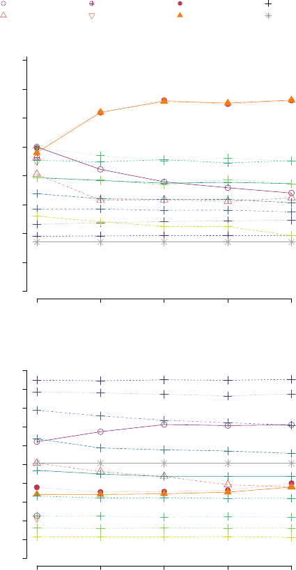
C. Influence of the number of observations
Let us now study the influence of the number of
observations on the approaches performances. The means
scores of precision and recall according to n are presented
in Figure 5 for all the approaches. Note that the approaches
pc KCI and fci KCI were only tested for n = 100 for
computational reasons. As for the previous experiments, few
simulations were removed. However, for all n considered, the
percentage of removed simulations was less or equal to 3%
of all simulations.
We observe that the correlation-based approaches remain
rather stable in terms of precision and recall except for τ ≤ 0.7
where the precision decreases with higher n. The approaches
pc gauss, f ci gauss loose precision when n increases. The
approaches pc KCI, fci KCI were only tested for n = 100
because they are in practice computationally demanding.
These approaches gave (for n = 100) both precision and
recall scores lower than our proposed approaches pc SCI,
fci SCI. This low performance is explained by the fact that
the default Gaussian kernel is not adapted to our simulated
data.
The proposed approaches both gain precision when n
increases up to 300 observations, then remain stable. In terms
of recall, our approaches are not sensible to n.
To summarize these experiments, the proposed approaches
reach the greater precision scores in the case where a latent
common cause is involved in the causal structure. Without
such a latent variable, our results stay competitive with the
correlation-based approaches. Our approach is sensitive to
the number of observations in terms of precision but stays

fuzzy pc gauss
fuzzy fci gauss
fuzzy pc SCI 20
fuzzy fci SCI 20
corr τ
random
(a) Legend.
0.0 0.2 0.4 0.6 0.8 1.0
0.0 0.2 0.4 0.6 0.8 1.0
recall
precision
0.1
0.2
0.3
0.4
0.5
0.6
0.7
0.8
0.9
(b) Without latent variable.
0.0 0.2 0.4 0.6 0.8 1.0
0.0 0.2 0.4 0.6 0.8 1.0
recall
precision
0.1
0.2
0.3
0.4
0.5
0.6
0.7
0.8
0.9
(c) With latent variable H .
Fig. 3: Mean scores of precision against mean scores of recall
for 6 approaches presented in the legend (3a). Results over
485 simulations in the case where there is no latent variable
(3b) and over 495 simulations in the case with a latent variable
(3c).
competitive with the other approaches even for a small number
of observations.
VI. CONCLUSION
Standard fuzzy rules would tend to associate premises with
consequences if the correlations are strong between premises
and consequences. However, a correlation should not be inter-
preted as causality. Indeed a correlation could be explained by
the presence of a common latent cause. This paper proposes
an innovative framework to represent causal statements where
the definitions of the cause and the effect are expressed by
0.0 0.2 0.4 0.6 0.8 1.00.0 0.2 0.4 0.6 0.8 1.0
pc gauss
pc SCI 20
fci gauss
fci SCI 20
corr 0.1
corr 0.2
corr 0.3
corr 0.4
corr 0.5
corr 0.6
corr 0.7
corr 0.8
corr 0.9
random
(a) Precision
0.0 0.2 0.4 0.6 0.8 1.00.0 0.2 0.4 0.6 0.8 1.0
pc gauss
pc SCI 20
fci gauss
fci SCI 20
corr 0.1
corr 0.2
corr 0.3
corr 0.4
corr 0.5
corr 0.6
corr 0.7
corr 0.8
corr 0.9
random
(b) Recall
Fig. 4: Boxplots of precision (4a) and recall (4b) scores.
Diamond shape inside boxplots correspond to the mean scores
presented in Fig 3.
fuzzy sets. Straightforwardly, these statements allow defining
causality-based fuzzy rules. Compared to standard fuzzy rules,
the causality-based fuzzy rules are not only designed for
prediction. They also allow a better understanding of a system.
Indeed causality is a key notion to reach the level of human
intelligence. Thus, our rules can be useful in many scientific
domains where it is necessary to provide insights concerning
a system.
The proposed approach enables the generation of causality-
based fuzzy statements from crisp observations. It performs
constraints-based causal discovery algorithms like PC of FCI,
combined with entropy-based conditional independence testing
before data discretization. The causality research is refined
to consider the different constraints specific to the fuzzy rule
generation context, by preventing some causal links.
Experiments on simulations were performed, in the presence
of a latent common cause and without any latent variable. The
ability to recover the causal links was evaluated in terms of
precision and recall for our approach and alternative ones. The
proposed approach obtained competitive scores of precision
and recall in the case where no latent variable is involved. In
the case where there is a latent common cause, our approach
obtained better performances in terms of precision, than the
considered state-of-the-art and correlation-based approaches.
fuzzy pc gauss
fuzzy fci gauss
fuzzy pc KCI
fuzzy fci KCI
fuzzy pc SCI 20
fuzzy fci SCI 20
corr τ
random
(a) Legend.
0.1
0.1
0.1
0.1
0.1
0.2
0.2
0.2
0.2
0.2
0.3
0.3
0.3
0.3
0.3
0.4
0.4
0.4
0.4
0.4
0.5
0.5
0.5
0.5
0.5
0.6
0.6
0.6
0.6
0.6
0.7
0.7
0.7
0.7
0.7
0.8
0.8
0.8
0.8
0.8
0.9
0.9
0.9
0.9
0.9
100 200 300 400 500
0.0
0.1
0.2
0.3
0.4
0.5
0.6
0.7
0.8
n
precision
(b)
0.1
0.1
0.1
0.1
0.1
0.2
0.2
0.2
0.2
0.2
0.3
0.3
0.3
0.3
0.3
0.4
0.4
0.4
0.4
0.4
0.5
0.5
0.5
0.5
0.5
0.6
0.6
0.6
0.6
0.6
0.7
0.7
0.7
0.7
0.7
0.8
0.8
0.8
0.8
0.8
0.9
0.9
0.9
0.9
0.9
100 200 300 400 500
0.0
0.1
0.2
0.3
0.4
0.5
0.6
0.7
0.8
0.9
1.0
n
recall
(c)
Fig. 5: For the 8 approaches presented in the legend (5a),
mean scores of precision 5b and recall 5c as a function of
the number of observations n. All results over at least 485
simulations.
The first perspective of this work is to apply our proposition
to a real application in collaboration with experts. Then,
another task will be to work on the fuzzy set extraction step.
We plan to optimize the interpretability and causal relevance
of fuzzy sets. We also plan to consider the joint effects that
correspond to the case of “and”/“or” combinations in the fuzzy
premises. However, this introduction of the joined effect in our
procedure of fuzzy causal discovery would lead to an increase
in complexity that would need to be optimized.
REFERENCES
[1] J. Pearl, “Theoretical impediments to machine learning with seven sparks
from the causal revolution,” arXiv preprint arXiv:1801.04016, 2018.
[2] C. P. Agueda, “Causality in sciencie,” Pensamiento Matem
´
atico, no. 1,
p. 12, 2011.
[3] E. Sanchez, “Solutions in composite fuzzy relation equations: applica-
tion to medical diagnosis in brouwerian logic,” in Readings in Fuzzy
Sets for Intelligent Systems, pp. 159–165, Elsevier, 1993.
[4] H. Hajri, J.-P. Poli, and L. Boudet, “Towards monotonous functions
approximation from few data with gradual generalized modus ponens:
Application to materials science,” in 2021 IEEE 33rd International
Conference on Tools with Artificial Intelligence (ICTAI), pp. 796–800,
IEEE, 2021.
[5] J. Pearl, Causality. Cambridge university press, 2009.
[6] R. Guo, L. Cheng, J. Li, P. R. Hahn, and H. Liu, “A survey of learning
causality with data: Problems and methods,” ACM Computing Surveys
(CSUR), vol. 53, no. 4, pp. 1–37, 2020.
[7] C. Glymour, K. Zhang, and P. Spirtes, “Review of causal discovery
methods based on graphical models,” Frontiers in genetics, vol. 10,
p. 524, 2019.
[8] P. Spirtes, C. N. Glymour, R. Scheines, and D. Heckerman, Causation,
prediction, and search. MIT press, 2000.
[9] D. Colombo, M. H. Maathuis, M. Kalisch, and T. S. Richardson,
“Learning high-dimensional directed acyclic graphs with latent and
selection variables,” The Annals of Statistics, pp. 294–321, 2012.
[10] P. L. Spirtes, C. Meek, and T. S. Richardson, “Causal inference in
the presence of latent variables and selection bias,” arXiv preprint
arXiv:1302.4983, 2013.
[11] D. M. Chickering, “Optimal structure identification with greedy search,”
Journal of machine learning research, vol. 3, no. Nov, pp. 507–554,
2002.
[12] S. Shimizu, P. O. Hoyer, A. Hyv
¨
arinen, A. Kerminen, and M. Jordan,
“A linear non-gaussian acyclic model for causal discovery.,” Journal of
Machine Learning Research, vol. 7, no. 10, 2006.
[13] P. Bonissone, M. Henrion, L. Kanal, and J. Lemmer, “Equivalence and
synthesis of causal models,” in Uncertainty in artificial intelligence,
vol. 6, p. 255, Elsevier Science & Technology, 1991.
[14] G. Schwarz et al., “Estimating the dimension of a model,” Annals of
statistics, vol. 6, no. 2, pp. 461–464, 1978.
[15] D. Dubois and H. Prade, “Fuzzy relation equations and causal reason-
ing,” Fuzzy sets and systems, vol. 75, no. 2, pp. 119–134, 1995.
[16] D. Dubois and H. Prade, “A glance at causality theories for artificial
intelligence,” in A Guided Tour of Artificial Intelligence Research,
pp. 275–305, Springer, 2020.
[17] D. Dubois and H. Prade, “An overview of ordinal and numerical
approaches to causal diagnostic problem solving,” Abductive reasoning
and learning, pp. 231–280, 2000.
[18] J. Dunn, “A graph theoretic analysis of pattern classification via tamura’s
fuzzy relation,” IEEE Transactions on Systems, Man, and Cybernetics,
no. 3, pp. 310–313, 1974.
[19] J. C. Bezdek, “Objective function clustering,” in Pattern recognition with
fuzzy objective function algorithms, pp. 43–93, Springer, 1981.
[20] D. Malinsky and D. Danks, “Causal discovery algorithms: A practical
guide,” Philosophy Compass, vol. 13, no. 1, 2018.
[21] P. Spirtes and R. Scheines, “Causal inference of ambiguous manipula-
tions,” Philosophy of Science, vol. 71, no. 5, pp. 833–845, 2004.
[22] K. Zhang, J. Peters, D. Janzing, and B. Sch
¨
olkopf, “Kernel-based
conditional independence test and application in causal discovery,” arXiv
preprint arXiv:1202.3775, 2012.
[23] K. Fukumizu, F. R. Bach, and M. I. Jordan, “Dimensionality reduction
for supervised learning with reproducing kernel hilbert spaces,” Journal
of Machine Learning Research, vol. 5, no. Jan, pp. 73–99, 2004.
[24] A. Marx and J. Vreeken, “Testing conditional independence on discrete
data using stochastic complexity,” in The 22nd International Conference
on Artificial Intelligence and Statistics, pp. 496–505, PMLR, 2019.
[25] M. Kalisch and P. B
¨
uhlmann, “Robustification of the pc-algorithm
for directed acyclic graphs,” Journal of Computational and Graphical
Statistics, vol. 17, no. 4, pp. 773–789, 2008.
[26] M. Kalisch and P. B
¨
uhlman, “Estimating high-dimensional directed
acyclic graphs with the pc-algorithm.,” Journal of Machine Learning
Research, vol. 8, no. 3, 2007.
