Seismic Noise Analysis System Using Power Spectral Density

Seismic Noise Analysis System Using Power Spectral

Density Probability Density Functions: A Stand-Alone

Software Package

By D. E. McNamara and R.I. Boaz

Open-File Report 2005-1438

U.S. Department of the Interior

U.S. Geological Survey

U.S. Department of the Interior

Gale A. Norton, Secretary

U.S. Geological Survey

P. Patrick Leahy, Acting Director

U.S. Geological Survey, Reston, Virginia 2006

For product and ordering information:

World Wide Web: http://www.usgs.gov/pubprod

Telephone: 1-888-ASK-USGS

For more information on the USGS—the Federal source for science about the Earth,

its natural and living resources, natural hazards, and the environment:

World Wide Web: http://www.usgs.gov

Telephone: 1-888-ASK-USGS

Contents

Abstract ..........................................................................................................................................................4

Section I: Introduction and Overview of Noise Analysis Methods................................................................ 4

Noise Analysis System Details....................................................................................................................... 6

Summary and Conclusions: Section I ..........................................................................................................12

References Cited........................................................................................................................................... 13

Acknowledgements ...................................................................................................................................... 13

Section II: System Description and Installation Instructions ....................................................................... 15

Figures

1. PDF example for LTX BHZ, with some artifacts and signals identified ................................................... 6

2. SDCO BHZ July 28, 2002, 06:00:00, PSD. Powers are averaged over full octaves in 1/8 octave

intervals. Center points of averaging are shown .............................................................................. 10

3. Histograms of powers, in 1dB bins, at four separate period bands for station AHID BHZ..................... 11

4. HLID - Typical ANSS station ~10km from Hailey Idaho .......................................................................14

iii

Seismic Noise Analysis System Using Power

Spectral Density Probability Density

Functions—A Stand-Alone Software Package

By D. E. McNamara and R.I. Boaz

Abstract

In this U.S. Geological Survey open-file report, we detail the methods and installation

procedures for a stand-alone noise analysis software package. The noise analysis system

is based on the calculation of the distribution of power spectral density using a

probability density function. Following the successful implementation of the noise

analysis system, at both the Incorporated Research Institutions in Seismology Data

management system in Seattle, Washington, and the Advanced National Seismic System

Data Collection Center in Golden, Colorado, we the system will be available to the

seismic community in a stand-alone form. This will allow users in the broader seismic

community the opportunity to perform their own analyses on data sets not held by either

of these two data centers. Potential users might include regional earthquake monitoring

network operators, portable experiment investigators and researchers and students

interested in the quality and noise characteristics of a particular data set. Results from this

noise analysis display the frequency dependent power distribution of the entire data set

and are useful for characterizing the performance of existing broadband stations, for

detecting operational problems, and for learning about sources of seismic noise within a

data set.

This report is divided in two sections. Section I describes how to acquire the noise

analysis software system and details data preparation and processing as well as the noise

analysis calculations and methods. Section II is a detailed description of the software

system. It will be useful to users interested in detailed installation instructions and a

complete description of the system directory structure and operations.

Section I: Introduction and Overview of Noise Analysis

Methods

A new stand-alone system for analyzing data quality is available to the seismology

community allowing users to evaluate the long-term seismic noise levels for broadband

seismic data in miniSEED format. The new noise processing software uses a probability

density function (PDF) to display the distribution of seismic power spectral density

(PSD) (PSD method after Peterson, 1993) and can be implemented against any

broadband seismic data with well known instrument responses. The software system is

currently running for routine noise monitoring at the United States Geological Survey’s

(USGS) Advanced National Seismic System (ANSS) National Operations Center (NOC)

Boaz Consultancy

and at the Incorporated Research Institutions in Seismology’s (IRIS) Data Management

Center ( DMC). For PDF plots from these two installations see:

http://geohazards.cr.usgs.gov/staffweb/mcnamara/ANSSPDFweb/ANSSPDFweb.html

and

http://www.iris.washington.edu/servlet/quackquery/

Software Availability

The new stand-alone software package is available on the world wide web (WWW)

and on the USGS ANSS anonymous ftp server. To download a compressed tar ball of the

software system, go to the following website and follow the downloading instructions.

http://geohazards.cr.usgs.gov/staffweb/mcnamara/Software/PDFSA.html

The download includes complete documentation on installing and running the noise

processing system. It also includes several reference documents on interpreting the noise

PDF plots (for example, McNamara and Buland, 2004).

Noise Analysis System Overview

This noise processing system is unique in that there is no need to screen the data

for earthquakes, system glitches, or general data artifacts as is commonly done in seismic

noise analysis. Instead with this new analysis, system transients map into a low-level

background probability while ambient noise conditions reveal themselves as high

probability occurrences. In fact, examination of artifacts related to station operation and

episodic cultural noise allows the user to estimate the overall station quality and a

baseline level of earth noise at each site. PDF noise plots are useful for characterizing the

current and past performance of existing broadband sensors, for detecting operational

problems within the recording system, and for evaluating the overall quality of data for a

particular station. The advantages of this new approach include:

(1) an analytical view representing the true ambient noise levels rather than a

simple absolute minimum,

(2) an assessment of the overall health of the instrument/station, and

(3) an assessment of the health of recording and telemetry systems.

Employing the algorithm used to develop the USGS Albuquerque Seismological

Laboratory (ASL) low noise model (LNM;

Peterson, 1993), we compute the PSD for

broadband data in the following manner. Hour-long, continuous, and over-lapping (50

percent) time-series segments are processed. There is no removal of earthquakes, system

transients and(or) data glitches. The instrument transfer function is removed from each

segment, yielding ground acceleration (for easy comparison to the LNM). Each hour-

long time series is divided into 13 segments, each about 15 minutes long and overlapping

by 75 percent, with each segment processed by removing the mean; removing the long

period trend; tapering using a 10 percent sine function; and transforming using an FFT

algorithm (Bendat and Piersol, 1971). Segments are then averaged to provide a PSD for

each 1-hour time series segment. For each channel, raw frequency distributions are

constructed by gathering individual PSDs in the following manner: binning periods in 1/8

octave intervals and binning power in 1 dB intervals. Each raw frequency distribution bin

is normalized by the total number of PSDs to construct a PDF. The probability of

occurrence of a given power at a particular period is plotted for direct comparison to the

Peterson high and low noise models (HNM, LNM) (see Fig. 1, LTX BHZ). Also

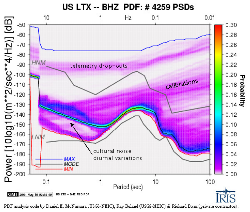
computed and plotted are the minimum (red line), mode (black line), and maximum (blue

line) powers for each period bin. A wealth of seismic noise information can be obtained

from this statistical view of broadband seismic noise.

Figure 1

Figure 1. PDF example for LTX BHZ, with some artifacts and signals identified. Station

LTX - Lajitas TX, was instrumental in the original Peterson Low Noise Model (Peterson,

1993); however, due to increased cultural noise (0.1-1s, 1-10Hz) the highest probability

power levels (mode, black line) are now significantly higher than the Peterson low noise

model (LNM). The minimum (red line) will approach the LNM <2 percent of the time

indicating that the station minimum does not reflect actual ambient noise conditions

across the whole spectrum. Instead, ambient noise conditions are better represented by

the highest probability mode (black line).

Noise Analysis System Details

Data Preparation and Processing

The approach of this noise analysis method differs from many previous noise studies

in that we make no attempt to screen the continuous waveforms to eliminate body and

surface waves from earthquakes or transients and instrumental glitches such as data gaps,

clipping, spikes, mass recenters, or calibration pulses. These signals are included in our

processing because they are low-probability occurrences that do not contaminate high-

probability ambient seismic noise observed in the PDFs (see below for details). In fact,

transient signals often are useful for evaluating station performance. Also, eliminating

this event-triggering and removal stage has the benefit of significantly reducing the PSD

computation time by simplifying data pre-processing.

The algorithm used to develop the Albuquerque Seismological Laboratory (ASL) new

low noise model (NLNM) and new high noise model (NHNM) (Peterson, 1993; Bendat

and Piersol, 1971) is used to calculate PSDs for all stations in this study. The processing

steps are detailed below.

Record length. Let a finite length seismic time series, u(t), have N evenly sampled

points at an interval of

t. For our analysis, we parse continuous time series, for each

station component, into 1-hour (T

=3600s) finite-length time series segments,

overlapping by 50 pecent, distributed continuously in time. Overlapping time series

segments are used to reduce variance in the PSD estimate (Cooley and Tukey, 1965). For

this example, we assume that for the broadband seismic data, each 3600s times series

segment is sampled at 40 sample per second (sps), such that

t••••••s, for a total

N=144,000 data points.

Preprocessing. The PSD preprocessing of each 1-hour time segment consists of

several operations. First, to significantly improve the Fast Fourier Transform (FFT) speed

ratio, by reducing the number of operations, the number of samples in the time series, N,

is truncated to the next lowest power of two, 2

, leaving N=131,072, thereby reducing the

series length such that T

=3276.8s. Second, in order to further reduce the variance of the

final PSD estimates, each roughly 1-hour time series record is divided into 13 segments,

overlapping by 75 percent, where the length of each new time series segment is now,

/4=819.2s with N=32,768=2

. The sample size N is chosen based on the longest

period of interest, T

, (lowest frequency, fl). In general, the record length, T

t, is

chosen such that it is 10 times the longest resolvable period, T

. Given this,T

,=1/f

/10=90s. The shortest period, Ts, (highest frequency, fh) is equivalent to the Nyquist

folding frequency, fc=1/2•t=20Hz, and is given by Ts = 1/fc

≤

1/fh

≤

0.05s.

Third, in order to minimize long-period contamination, the data are transformed to a

zero mean value, and any long period linear trend is removed by the average slope

method. If u

are the data values in the time series u(t) of length T

and N samples, the

data mean is given by:

(1)

mean

n=1

∑

Long period trend, T

, is defined as any frequency component whose period is longer

than the record length, T

, and is defined as:

(2)

Tlp =

t −

⎛

⎝

⎜

⎞

⎠

⎟

where 0

≤

and

(3)

⎛

⎝

⎜

⎞

⎠

⎟

2Tr

⎛

⎝

⎜

⎞

⎠

⎟

u(t)dt − u(t)dt

∫

2Tr

∫

⎡

⎣

⎢

⎤

⎦

⎥

If trends are not eliminated in the data, large distortions can occur in spectral

processing by nullifying the estimation of low frequency spectral quantities. Subtracting

(1) and (2) from the original time series, u(t), produces a new time series , u(t), that has

zero mean and long period trends removed: (4)

(

)

−

mean

−

Tlp

Fourth, to suppress side lobe leakage in the resulting FFT, a 10 percent sine taper is

applied to the ends of the time series, x(t). We define a new tapered time series, y(t), such

that:

y(t) = x(t) * sin(••••r * t) 0

≤

Tr/10

y(t) = x(t) Tr/10

≤

(Tr-Tr/10) (5)

y(t) = x(t) * sin(••••r * (Tr-t)) (Tr-Tr/10)

≤

Tr.

Tapering the time series has the effect of smoothing the FFT and minimizing the effect of

the discontinuity between the beginning and end of the time series. The time series

variance reduction can be quantified by the ratio of the total power in the raw FFT to the

total power in the smoothed filter (1.142857) and will be used to correct absolute power

in the final spectrum (Bendat and Piersol, 1971).

Power Spectral Density

The standard method for quantifying seismic background noise is to calculate the

noise PSD. The most common method for estimating the PSD for stationary random

seismic data is called the direct Fourier transform or Cooley-Tukey method (Cooley and

Tukey, 1965). The method computes the PSD via a finite-range fast Fourier transform

(FFT) of the original data and is advantageous for its computational efficiency.

The finite-range Fourier transform of a periodic time series y(t) is given by:

(6)

Y( f ,T ) = y(t)

∫

− i2

where the number of frequency amplitude estimates nfft=(N/2)+1=16385. For discrete

frequency values, f

, the Fourier components are defined as:

(7)

Yk =

k,T )

For , f

=k/N•t when k = 1, 2, …, N-1.

Hence, using the Fourier components defined above, the total power spectral density

estimate is defined as: (8)

k =

As is apparent from (8), the total power, P

, is simply the square of the amplitude

spectrum with a normalization factor of 2

t/N. The PSD process is repeated for each of

the 13 separate overlapping time segments within the one-hour record. After all 13

segment PSD estimates are computed, powers are averaged for q=13 separate time

segments, where each time segment is of length T

. The final smooth PSD estimate is

given by:

(9)

Pk =

k,1

+ P

k,2

+... + P

k ,q

(

)

where P

k,q

is the raw estimate at frequency f

of the qth time segment. Due to segment

averaging, the quantity P

has 2q=26 degrees of freedom giving a 95 percent level of

confidence that the spectral point lies within –2.14dB to +2.87dB of the estimate

(Peterson, 1993).

At this point we correct P

for the 10 percent sine taper applied earlier in the

processing such that P

= P

*1.142857 and then deconvolve the seismometer instrument

response by dividing the PSD, P

, estimate by the instrument transfer function to

acceleration, in the frequency domain. Finally, we convert the smoothed PSD estimate

into decibels (dB) with respect to acceleration (m/s

)

/Hz, for direct comparison to the

NLNM,by:

= 10*log

). (10)

Limitations. The PSD technique described above provides stable spectra estimates

over a broad range of periods (0.05-90s); however, it suffers from poor time resolution

due to the long transforms and requires hundreds to thousands of hours of data to compile

good statistics for the PDFs. For better resolution at shorter periods, a larger number of

shorter records should be analyzed. Future work will investigate methods to improve

resolution of higher frequencies.

Probability Density Functions

Our goal is to get a sense of the true variation of noise at a given station. We do this by

generating seismic noise PDFs from the PSDs processed by using the methods discussed

in the previous section. In order to adequately sample the PSDs, full octave averages are

taken in 1/8 octave intervals. This procedure reduces the number of frequencies by a

factor of 169 from nfft=16,385 to 97. Thus, power is averaged between a short period

(high frequency) corner, T

, and a long period (low frequency) corner of T

=2*T

, with a

center period, T

, such that T

=sqrt(T

) is the geometric mean period within the octave.

The geometric means are evenly spaced in log space. The average power for that octave,

period range from T

to T

, is stored with the center period of the octave, T

, for future

0.125

analysis. T

is incremented by one 1/8 octave such that T

= T

*2 , to compute the

average power for the next period bin. T

and T

are recomputed, powers are averaged

within the next period range T

to T

, and the process continues until we reach the longest

resolvable period given the time series window length of the original data, T

/10 (Fig. 2).

This process is repeated for every 1-hour PSD estimate, resulting in thousands of smooth

PSD estimates for each station-component. Powers are accumulated in 1 dB intervals to

produce frequency distribution plots (histograms), for each period (Fig. 3).

Period (sec)

PSD 10*log10 m**2/s**4/Hz dB

-180

-160

-140

-120

-100

NLNM

NHNM

SDCO BHZ July 28, 2002 06:00:00 PSD

Figure 2. SDCO BHZ July 28, 2002, 06:00:00, PSD. Powers are averaged over full

octaves in 1/8 octave intervals. Center points of averaging are shown.

500

100

200

300

400

-200 -180 -160 -140 -120 -100 -8

Power [10log10(m**2/s**4)] dB

number of occurrences

0.1 sec

1.0 sec

10.0 sec

100.0 sec

Period

Figure 3. Histograms of powers, in 1dB bins, at four separate period bands for station

AHID BHZ.

The next step is to plot the distribution of powers per period, as observed in figure 3,

using a probability density function (PDF). The PDF, for a given center period, T

, can

be estimated as:

P(T

) = N

PTc

(11)

where N

PTc

is the number of spectral estimates that fall into a 1 dB power bin, P, with a

range from –200 to –80 dB, and a center period, T

. N

is the total number of spectral

estimates over all powers with a center period, T

. We then plot the probability of

occurrence of a given power at a particular period for direct comparison to the high and

low noise models (Figs. 1 and 4) (Peterson, 1993). We also compute and plot the

minimum, mode, and maximum powers for each period bin. A wealth of seismic noise

information can be obtained from this statistical view of broadband PDFs as discussed in

the following section.

Characterizing Sources of Noise and Signal in the PDFs

Cultural Noise. The most common source of seismic noise is from the actions of

human beings at or near the surface of the Earth. This often is referred to as “cultural

noise” and primarily originates from the coupling of traffic and machinery energy into

the earth. Cultural noise propagates mainly as high-frequency surface waves (>1-10Hz,1-

0.1s) that attenuate within several kilometers in distance and depth. For this reason,

cultural noise generally is significantly reduced in boreholes, deep caves, and tunnels.

Cultural noise shows very strong diurnal variations and has characteristic frequencies

depending on the source of the disturbance (Figs. 1 and 4). Another source of noise with

a strong diurnal is from thermal instabilities. Heating during the day and cooling at night

can cause ground fluctuations that induce tilt and long-period noise.

Earthquakes. Our approach differs from many previous noise studies in that we make

no attempt to screen the continuous waveforms to eliminate body and surface waves from

naturally occurring earthquakes. Earthquake signals are included in our processing

because they are low-probability occurrences even at low power levels (small magnitude

events) compared to the ambient conditions at the seismic station. We are interested in

the true noise that a given station will experience; therefore we include all input signals.

For example, including earthquakes tells us something about the probability of

teleseismic signals being obscured by small local events as well as various noise sources.

Large teleseismic earthquakes can produce powers above ambient noise levels across the

entire spectrum and are dominated by surface waves >10s, while small events dominate

the short period, <1s. Earthquakes are observed in the PDFs as low probability smeared

signal at short and long periods (Fig. 4).

System Artifacts. Since we make no attempt to screen waveforms for system

transients such as data gaps and sensor glitches, the PDF plots contain numerous system

generated artifacts that can be very useful for network quality-control purposes. We have

attempted to determine the source of several coherent, high power, low-probability noise

artifacts in the PDF plots. Several artifacts in the PDFs are easily explained and may be

useful to the network operator. For example, data-gaps (due to telemetry dropouts) and

automatic mass recenters (necessitated by “drift” in sensor mass position) are easily

identifiable in the PDFs. Should the probability of mass recentering and(or) telemetry

dropouts drastically increase, a remote network operator could readily diagnose the

problem (Figs. 1 and 4). Additional features and artifacts observed in the PDFs are

described online at:

http://geohazards.cr.usgs.gov/mcnamara/PDFweb/Noise_PDFs.html

and in McNamara and Buland (2004).

Summary and Conclusions: Section I

We have presented a new method for more realistically evaluating ambient seismic

noise levels at a station based on the PSD methods used to generate the NLNM of

Peterson (1993). This approach is useful because seismic stations exhibit considerable

variations in noise levels as a function of time of day, season, location, and installation

type. This type of information is not readily observed when only minimum noise levels

are analyzed. The results of this type of background noise analysis are useful for

characterizing the performance of existing stations, for detecting operational problems,

and should be relevant to the future siting of broadband seismic stations. Details on

software system installation and operations will be discussed in Section II.

References Cited

Bendat, J.S. and A.G. Piersol, 1971, Random data: analysis and measurement procedures.

John Wiley and Sons, New York, 407p.

Cooley, J.W., and J. W. Tukey, 1965, An algorithm for machine calculation of complex

Fourier series, Math. Comp., 19, p. 297-301.

McNamara, D.E. and R.P. Buland, 2004,

Ambient Noise Levels in the Continental

United States

, Bull. Seism. Soc. Am., 94, 4, 1517-1527.

Peterson, J., 1993, Observation and modeling of seismic background noise,

U.S. Geol.

Surv. Tech. Rept., 93-322

, 1-95.

Wessel, P. and W. Smith, 1991, Free software helps display data, EOS, 72, 445-446.

Acknowledgements

The algorithm and initial software was first developed by Dan McNamara and Ray

Buland, with contributions from Harold Bolton and Paul Earle, at the United States

Geological Survey (USGS) as a part of the ANSS quality-control (QC) system. Further

development, supported by IRIS through funds it receives from the National Science

Foundation (NSF) allowed for Richard Boaz to develop the system for implementation

against the real-time BUD dataset and the real-time data stream at the USGS ANSS

NOC. Additional support was provided by the USGS to produce the stand-alone software

package discussed in this report. PDF plots are generated with the GMT plotting tools

(Wessel and Smith, 1991). Appropriate citation for this noise analysis method is

McNamara and Buland (2004) (see references).

Figure 4. HLID - Typical ANSS station ~10km from Hailey Idaho. Automobile traffic

along a dirt road only 20 meters from station HLID creates a 20-30dB increase in power

at about 0.1 sec period (10Hz). This type of cultural noise is observable in the PDFs as a

region of low probability at high frequencies (1-10Hz, 0.1-1s). Body waves occur as low

probability signal in the 1-sec range while surface waves are higher power at longer

periods. Automatic mass recentering and calibration pulses show up as low probability

occurrences in the PDF.

Section II: System Description and Installation Instructions

Table of Contents

Introduction __________________________________________________________ 1

Quick Install _________________________________________________________ 1

Audience ____________________________________________________________ 1

Scope _______________________________________________________________ 1

Acknowledgments _____________________________________________________ 1

Authorship ___________________________________________________________ 1

References ___________________________________________________________ 1

PDF Analysis System Overview____________________________________________ 2

Description __________________________________________________________ 2

Requirements_________________________________________________________ 2

Hardware __________________________________________________________ 2

Software ___________________________________________________________ 3

PDF Source Code Organization __________________________________________ 3

Input and Output Files ___________________________________________________ 3

Input________________________________________________________________ 3

Output ______________________________________________________________ 5

System Configuration ____________________________________________________ 5

Data Directories_______________________________________________________ 6

MiniSeed Data Directory and Files ______________________________________ 6

Response File Directory_______________________________________________ 6

Web Directory ______________________________________________________ 7

Script Variables _______________________________________________________ 8

Source Code Header File Modification_____________________________________ 8

System Compilation and Installation ________________________________________ 8

Compilation __________________________________________________________ 8

Compiler Options____________________________________________________ 8

Installation ___________________________________________________________ 9

PDF System Execution ___________________________________________________ 9

Channel-Specific Shell Script ____________________________________________ 9

Overall Execution ____________________________________________________ 10

xecution Features ___________________________________________________ 10

Error Processing______________________________________________________10

Release Notes _________________________________________________________ 11

Current Limitations ___________________________________________________ 11

Version Control ______________________________________________________ 11

Version 1.1 ________________________________________________________ 11

Appdendix I – File Formats ______________________________________________ 11

Djjj.bin File _________________________________________________________ 11

Hour.idx File ________________________________________________________ 11

Hjjj.bin File _________________________________________________________ 12

PDFAnalysis.bin File _________________________________________________ 12

PDFAnalysis.inf File __________________________________________________ 12

PDFanalysis.sts File __________________________________________________ 12

PDFAnalysisSR.bin File _______________________________________________ 13

Appendix II – Installation and Configuration Checklist__________________________ 1

PDF Analysis System – Stand Alone Installation

Introduction

Following from the successful implementation of the PDF Noise Analysis System at the IRIS DMC in

Seattle, Wash., and at the NEIC in Golden, Colo., it is desired to provide the system to the seismic

community in a stand-alone form. The stand-alone software package will allow seismic community users

the opportunity to perform their own analyses against data sets not held by the two data centers.

Quick Install

If the time required to read and understand this document in total is unavailable (but you’d like it installed

and working as quickly as possible), you must at least read the sections System Configuration, System

Compilation and Installation, and PDF System Execution and follow the steps outlined there. Where

problems occur, be certain to consult the other various sections of this document that may provide further

information to solve your issue.

Audience

This document is intended for all users of the siesmic community with an interest in producing noise

analyses of seismic data following the algorithm laid out by McNamara and Buland of the USGS ANSS

National Operations Center (NOC) in Golden, Colo.

Scope

This document is limited to the technical aspects of the PDF Analysis System: installation, configuration,

and execution. As such, it does not treat the functional aspects of the system: methodologies, algorithm,

philosophy, interpretation possibilities, usage of results, etc. For a complete discussion of these and more,

please consult the various documents listed below.

Acknowledgments

The following parties have significantly contributed to the development of this system and are hereby

acknowledged thus:

Party Contribution

Ray Buland and Daniel

McNamara (of USGS

NEIC, Golden, CO)

Provided the original algorithm and proof-of-concept implementation

USGS NEIC Provided the funds for original development of algorithm.

NSF Provided funds for original system development of generic implementation at

the IRIS Data Management Center (Seattle, Wash).

IRIS Sponsored the development of the generic implementation at the DMC.

Bruce Weertman (of

IRIS)

Responsible for integration of the PDF system within the IRIS DMC’s Quack

framework.

Authorship

This document and the PDF analysis system was written by Richard Boaz (of Boaz Consultancy:

http://www.boazconsultancy.com) and Dan McNamara (USGS). Any and all comments and(or) bug reports

are welcome and are encouraged to be forwarded to

riboaz@xs4all.nl.

References

The following table provides various references which may be of interest to the reader:

Description Name Location

Original Abstract

(Adobe pdf)

Ambient Noise Levels in the

Continental United States

PDF Stand-Alone distribution docs directory

Power Point

Presentation

Noise Based Detection

Method for the ANSS

PDF Stand-Alone distribution docs directory

Discussion Paper

(Adobe pdf)

Determining True Global

Ambient Noise

PDF Stand-Alone distribution docs directory

PDF Analysis

Interpretation (html

document)

Ambient Noise Probability

Density Functions

PDF Stand-Alone distribution docs directory

PDF Analyses at the

USGS NEIC

USGS/ANSS Noise Monitor

http://geohazards.cr.usgs.gov/staffweb/mcnamara/

ANSSPDFweb/ANSSPDFweb.html

PDF Analyses at the

IRIS DMC

DMC QUACK Information

Query

http://www.iris.washington.edu/servlet/quackquery

PDF Analyses at the

IRIS DMC (US

Array)

DMC QUACK Information

Query

http://www.iris.washington.edu/servlet/quackquery

_us

Description

The PDF Analysis system is comprised of three separate processing components:

1. An analysis program (written in C), responsible for producing analysis statistics for a single

channel;

2. A shell program (using GMT) to convert the analysis results produced in step 1 to a plot, in the

form of a postscript format file;

3. Image manipulation (using ImageMagick) commands to convert the postscript file created in step

2 to an actual graphical image (.png format).

Execution is provided in the form of a shell script per channel to analyze, responsible for calling each of

these components in turn (see section PDF System Execution below for details).

Requirements

Hardware

No specific hardware requirements exist, per se. The program will execute on any platform supporting a C

compiler in addition to the other software requirements listed below.

Depending on which compile time output option is chosen (please see section System Compilation and

Installation: Compilation: Compile Options for a complete discussion of these options and their effects),

disk storage requirements are approximately the following (per channel analyzed):

Output Option

Maximum disk

storage requirement

No Daily or Hourly .bin output 5 Mb

Only Daily .bin output 15 Mb

Both Daily and Hourly .bin output 50 Mb

Software

The following table defines the software dependencies currently en force:

Software Version Description Available at

C Compiler User preference Compiler (program

developed under gcc)

http://gcc.gnu.org/

Scripting Bash shell Scripting tools Local machine executing analysis

GMT Latest available Plotting tool

http://gmt.soest.hawaii.edu/

ImageMagick Latest available Image manipulation tool

http://www.imagemagick.org/

PDF Source Code Organization

The following table defines the directories and files which make up the source tree of the PDF Analysis

System:

Directory/File Description

PDF Root system directory

PDF/PROD Production directory containing production relevant files

PDF/PROD/bin Directory containing shells and executables,

PDF/PROD/script Directory containing executable scripts

PDF/PROD/support Directory containing all necessary production support files

PDF/PROD/helper Directory containing helper scripts (system mgmt, etc.)

PDF/src Directory holding all source code:

• PDF analysis program

• GMT plotting script

• Execution scripts

PDF/src/vx.x.x Directory holding all source code for version x.x.x of the system

PDF/src/ vx.x.x/analysis Source code directory of analysis program (C code)

PDF/src/ vx.x.x/analysis/mseed Miniseed data file reader source code - as library to main()

PDF/src/ vx.x.x/analysis/resp Instrument response interpreter source code - as library to main()

PDF/src/ vx.x.x/GMT Directory holding GMT source code - scripts and support files

PDF/src/ vx.x.x/script Directory holding execution scripts

Input and Output Files

Input

The following table defines the directories and files which are required input, see sections System

Configuration and PDF System Execution for full description of specification and use:

Directory/File Description

Data Directory Directory holding the miniseed data files to be analyzed.

Note: All data files requiring analysis as part of a single execution

must reside in this single directory.

Miniseed Data Files Files to analyze, miniseed format only.

Analysis Directory Directory holding all output files.

See section Output for a complete description.

Response File Directory Directory holding response files for channels being analyzed.

See section System Configuration for a complete discussion on set-

up.

RESP.NTW.STN.LOC.CHN The file holding the response information for the instrument and

channel. This must be formatted as for input to the evresp() function

(format as produced by the rdseed program).

Where:

NTW is the network name

STN is the station name

LOC is the location identifier

CHN is the channel identifier

Output

The following table defines the directories and files which are created in the course of the PDF Analysis

execution. All are located as subdirectories to the analysis directory defined in the section Input above and

are automatically created in the course of execution. Please consult Appendix I – File Formats for a

detailed description of their contents.

Directory/File Description

NTW.STN.LOC.CHN.png Graphical representation of analysis.

Yyyyy Directory holding daily PSD .bin files, by year

Where:

yyyy is the year

Yyyyy/HOUR Directory holding the hourly PSD .bin files

LOG Directory holding the various log files created during the course of

execution.

wrk Directory holding various work files

Yyyyy/Djjj.bin Files holding individual day's PSD analysis results (currently unused,

for future use).

Where:

jjj is the julian day

Yyyyy/HOUR/hour.idx Index file to Hjjj.bin file.

Yyyyy/HOUR/Hjjj.bin Files holding individual hour's PSD analysis results (currently unused,

for future use).

LOG/NTW.STN.LOC.CHN.log Log file of analysis program.

LOG/plotGMT.log Log file of GMT plotting program.

LOG/convert.log Log file of ImageMagick convert program, nothing output for normal

execution.

LOG/NTW.STN.LOC.CHN.yyyy.jj

j.err

Analysis program error file, by year and julian day.

LOG/PDFanalysis.skp File listing those days when problems occurred, information only.

wrk/PDFanalysis.bin Cumulative dB-based .bin file, results to graph are contained here.

wrk/PDFanalysis.inf Information file holding various analysis settings.

wrk/PDFanalysisSR.bin Cumulative period-based .bin file.

Where:

SR is the sample rate of the channel

wrk/PDFanalysisSR.inf Information file as before, sample-rate specific.

wrk/PDFanalysis.sts File holding various statistics for analysis results, input to GMT.

wrk/PDFanalysis.ps GMT postscript file output, deleted upon conversion to .png file.

wrk/pdf.grd GMT temp file, deleted upon completion of GMT step.

System Configuration

Configuration of the PDF system amounts to the setup of various directories and script variables. This

section lays out these requirements for the PDF system setup to result in a successful installation and

subsequent execution. Failure to define these precisely as described herein will result in a nonfunctioning

system.

Appendix II provides a checklist for each parameter and variable which must be defined as part of system

setup. Please print, define the values accordingly, and supply them in their proper location.

Data Directories

MiniSeed Data Directory and Files

A directory is required to contain the miniseed data files to be analyzed. This directory and the miniseed

data files must adhere to the following:

1. All miniseed data files representing a single channel’s worth of waveform data, for all time, must

be contained within the same directory.

2. All miniseed data files must contain exactly (or as close to) 1 day’s worth of data, from 00:00

hours to 24:00 hours.

3. The directory structure must conform to the following conventions:

DATAROOT/NTW/STN

Where

DATAROOT is the root directory of the miniseed data files (script variable of such specified

below)

NTW is the name of the network

STN is the name of the station

4. The name of the miniseed file itself must conform to the following naming convention:

STN. NTW.LOC.CHN.yyyy.jjj

Where

STN is the name of the station

NTW is the name of the network

LOC is the location identifier

CHN is the channel identifier

yyyy is the year of the data file

jjj is the julian day of the data file

(Note: Where no location identifier exists, field should be null. This would render, for example, a

filename for station ATKA and network AK as: ATKA.AK..BHE.2004.261)

Assuming your directory structure and miniseed data files do not naturally conform to these requirements,

this directory structure and filenaming convention can be easily accommodated for through the following:

• Create the fixed directory structure itself: DATAROOT/NTW/STN

• For each miniseed data file, create softlinks (ln –s) to the actual/real miniseed data files such that

the naming convention above is adhered to.

Further, this can be automated via a script rendering this requirement as trivial as possible. Please see the

script linkMseed.US (located in pdf/PROD/helper/linkmseed) for an example and modify as necessary.

Because the filenaming convention uniquely identifies the channel of data, this directory may contain all

miniseed data file for all channels of a station. It is not necessary to create separate directories for each

channel, rather, a separate directory only for the station itself and containing the miniseed data files for all

channels.

Response File Directory

A directory must exist containing all response files used to deconvolve the signal back to absolute ground

motion in the course of analysis. This directory and the files themselves must adhere to the following:

1. The directory may be specified as per user desires/requirements. No specific directory structure

requirement exists. The directory holding these response files must be specified in two places: in

the script variable RESPDIR (see section Script Vaiables below), and within the PDFuser.h file

of the PDF analysis program source code (see section Source Code Header File Modification

below).

2. The filename of the response file must conform to the following naming convention:

RESP.NTW.STN.LOC.CHN

Where

RESP is exactly as specified: RESP

NTW is the name of the network

STN is the name of the station

LOC is the location identifier

CHN is the channel identifier

(Note: This naming convention follows from the response file output generated by the rdseed

program. As before, where no location identifier exists, field should be null.)

3. The internal format of the response file information must conform to the format produced by the

rdseed program, subsequently readable by evresp().

Web Directory

A directory must be created to collect all .png files created during the course of execution. The .png files

are contained in the analysis directory for the channel being analyzed, making collective viewing annoying

since all are held within disparate directories. This annoyance is alleviated through the existence of this

directory.

Create a directory for these to be contained in and define this location in the .vars-user file. With this

directory, the last action in the course of analysis is for a softlink to be created in this directory pointing to

the .png file found in the analysis directory.

Additionally, if it is desired to publish the results, it is this directory that can be made available to the web

in whatever manner/means appropriate.

Script Variables

The following script variables are installation specific and must be predefined by the user and provided in

the shell script file .vars-user (located in directory PDF) before the system can be installed. Failure to do

so will result in a non-functioning system.

Script variable name Description

PDFROOT Root directory of PDF analysis system (directory holding the .vars-user file)

WEBDIR Directory of collected .png files

RESPDIR Directory holding response files

DATAROOT Root directory of miniseed data files (parent to NTW/STN)

STATSROOT Root directory of PDF analysis results/statistics

GMTROOT GMT installation root directory

IMROOT ImageMagick installation root directory

Source Code Header File Modification

The sole configuration requirement within the source code of the PDF analysis program is the following

#define parameter to be specified: (Note: this must be the same as defined as part of the Script Variables

above.)

#define parameter Description Location

#define RESPDIR Directory holding response files,

inside quotes “”.

PDF/src/vx.x.x/analysis/PDFuser.h

System Compilation and Installation

Compilation

Compilation of the PDF Analysis program employs straightforward C/Unix standards, that is, a C compiler

and make. In addition to the analysis portion of the program, there are two subdirectories of libraries

requiring compilation as well. As such, a script is provided that will traverse each of these subdirectories,

making the dependent libraries in turn. This script is located in the PDF Analysis source directory and

conforms to the following invocation specifications:

makesh [ clean | all ]

where

clean will execute make clean, removing all dependent libraries and object files.

all will execute make all in each directory of the PDF analysis program, creating all dependent

libraries and object files necessary to ultimately link the PDF analysis executable.

Alternatively, the program may be built when installing the system as a whole, alleviating the need to

compile and link by hand. Please see the section Installation below for details.

Compiler Options

Two compile-time options exist for the PDF Analysis program. Namely, defining whether or not daily

and(or) hourly PSD information is output. (Please see section Requirements: Hardware for detailed

overall disk storage requirements.)

With daily PSD information output, cumulative .bin files are generated for each day analyzed (amounting

to ~30Kb/day/channel analyzed).

With hourly PSD information output, .bin files are generated for each hour analyzed (amounting to

~100Kb/day/channel analyzed).

The system is delivered, by default, to output daily and hourly .bin files. Output of this data is anticipated

to be used in future versions of the software, such that existence of these files will allow PDFs to be

produced for specific user-defined time periods. For example, a PDF graph representing only the months

of January thru March or a PDF graph representing all months but only between the hours of 6AM and

6PM.

If it is anticipated that these more specific sorts of analyses will be of interest, no action is required, daily

and hourly .bin files will be generated.

If this is not desired, or disk space is an issue, both daily and hourly .bin file generation may be suppressed.

The following table defines these compile time options:

Compiler option Effect

-DNO_DAILY_PSD No daily PSD .bin files output

-DNO_HOURLY_PSD

No hourly PSD .bin files output

Either or both (they are mutually independent) of these options can be specified in the CFLAGS section of

the Makefile for the main PDF Analysis program. The resulting executable will subsequently NOT output

incremental PSD information.

Since these are compiler options, these settings have a system-wide influence, that is, these options cannot

be implemented on a per channel basis. (One way around this, however, would be to install more than a

single system.)

Installation

Installation is provided via the shell script installPDF located in the directory PDF and provides for the

following functionality:

1. optionally compiles the PDF Analysis program,

2. copies all relevant files to the PROD directory, and

3. conforms to the following usages:

command: installPDF –h

output: Usage: install [-h] [make] version#

description: prints the usage for the command.

command: installPDF v1.1

output: Copying v1.1 executables and support files to PROD dir…

description: installs all relevant executables, scripts and support files for version# to the PROD

directory structure. (Note: command line argument version# must be as specified in the

PDF source directory structure.)

command: installPDF make v1.1

output: Compiling v1.1 PDF Analysis program…

Copying v1.1 executables and support files to PROD dir…

description: as for command installPDF v1.1, however, cleans and compiles the PDF analysis

program before copying and installing to the PROD directory structure (recommended

for first install since no object files exist as part of delivery).

PDF System Execution

System execution comes in the form of two scripts, executePDF and PDFscript (both located in

PDF/PROD/bin).

PDFscript is a shell script template used to create the individual channel-specific execution script. This

script is ultimately responsible for the PDF analysis execution of a specific channel.

The executePDF script executes all channel-specific scripts located in PDF/PROD/script in turn.

Channel-Specific Shell Script

Execution of the PDF Analysis System is provided in the form of a shell executable script (PDFscript)

responsible for carrying out the three steps of execution described in section PDF Analysis System

Overview: Description. This execution script is created by replacing various strings in the generic file

PDFscript with execution-specific values, thus creating a unique script for each channel to be analyzed.

This channel-specific executable shell can be easily created using the following shell script command:

makePDFscript NTW STN LOC CHN

where

NTW is the network name

STN is the station name

LOC is the location identifier (use -- for no location)

CHN is the channel identifier

This will create the channel-specific script to be executed, named NTW.STN.LOC.CHN.sh and saved to the

directory PDF/PROD/script. In addition, the analysis directory will be created if it does not exist (assuming

the STATSROOT directory exists).

Once this script has been created for a specific channel, it can be executed repeatedly (daily, weekly,

monthly, as desired) to update the analysis results.

Overall Execution

Executing the script executePDF will result in all scripts located in PDF/PROD/script to be executed in

turn. Specifically, it will execute all files having “.sh” as their filename suffix. Thus, individual analyses

can be turned on and off by renaming the suffix of the executable script in question.

A simple logfile of executePDF, detailing the channels analyzed, is generated and written to the file

PDF/PROD/LOG/PDF.log.

Further, this process may be automated by using the UNIX crontab command. At specified times, merely

execute the executePDF script, and all analyses will be performed and updated.

Execution Features

Please note the following features of the PDF analysis system:

1. Analysis is performed against all data files found in the specified data directory only up to and

until 2 days prior to analysis execution date. This allows for systems where data availability can

suffer up to 2 days of latency.

2. The program does cross the day boundary to analyze the last hour of data held within the miniseed

files. As such, the last file identified for analysis is not fully analyzed; it is treated in subsequent

executions.

3. When crossing the day boundary, program assumes data are coincident if ending time and starting

time of respective miniseed files differ by less than one sample (1) of time. Where data are

identified not to be coincident, an error message is output to the channel-specific log file.

Error Processing

Error handling is very much dependent on the type of error encountered. The following table lists the

major errors that may be encountered, how each is handled, and suggested follow-up action.

Error Type How handled User follow up

Response File not

found

Fatal Analysis execution suspended;

error message written to Log file

Provide proper response file, verify

naming convention is adhered to.

Response

Information not

found

Fatal Analysis execution suspended;

error message written to Log file

Provide file containing response

information for appropriate

date/time range, verify file format is

adhered to.

Error reading

miniseed data file

Nonfatal Analysis execution skips this

day of data; error message

written to day-specific error file

located in LOG directory of

analysis output.

Determine if miniseed data file can

be repaired.

Internal

Processing Error

Fatal Analysis execution suspended Contact riboaz@xs4all.nl with all

relevant information

No files ever

found to analyze

Nonfatal Program successfully executes

but nothing analyzed

Verify miniseed directory structure

and filenaming conventions are

adhered to.

Unable to create

or access

directories

Fatal Analysis execution suspended Confirm existence and access

permissions of directory in question.

Release Notes

Current Limitations

The limitations are defined to be:

1. Unable to analyze long period channels, limited to 20 samples/sec or more,

2. unable to provide analysis for user-defined time periods, only analysis of all data available is

currently provided for,

3. output provided to end-user currently limited to .png graphical file format, and

4. unable to analyze any data prior to the last day analyzed. This means that the program cannot fill

in gaps nor replace the results of previously analyzed data. This will be treated in a future release.

Version Control

This section defines the current and historical releases of the PDF Analysis System.

Version 1.1

Release Date: 29 October 2004

Modifications

1. Stand-alone version created and made available for general release.

Appdendix I – File Formats

This appendix defines the formats of the various files produced by the PDF analysis system.

Djjj.bin File

Definition: Cumulative db-based .bin file holding daily PSD analyses for julian day jjj.

Directory: Yyyyy

Internal Format:

• Data Format: ASCII

• Individual lines each defining:

FREQ POWER #HITS

Where:

FREQ is the frequency (in Hz)

POWER is the power bin (in dB)

#HITS is the number of times

Hour.idx File

Definition: Index file to Hjjj.bin file, index defined by julian day and HH:MM start time of PSD.

Directory: Yyyyy/HOUR

Internal Format:

• Data Format: ASCII

• Individual lines each containing:

JDAY HH:MM REF

Where:

JDAY is the julian day

HH:MM is the hour and minute start time of the PSD

REF is the reference identifier, for accessing/extracting from the Hjjj.bin file

Hjjj.bin File

Definition: Cumulative db-based .bin file holding hourly PSD analyses for julian day jjj.

Directory: wrk

Internal Format:

• Data Format: ASCII

• Individual lines each containing:

REF FREQ POWER

Where:

REF is the reference identifier from the hour.idx file

FREQ is the frequency (in Hz)

POWER is the power bin (in dB)

PDFAnalysis.bin File

Definition: Cumulative db-based .bin file holding overall PSD probabilities for julian day jjj.

Directory: wrk

Internal Format:

• Data Format: ASCII

• Individual lines each defining:

FREQ POWER PROB

Where:

FREQ is the frequency (in seconds)

POWER is the power bin (in dB)

PROB is the normalized (to probability) number of hits

PDFAnalysis.inf File

Definition: Information file containing various settings/values pertaining to analysis.

Directory: wrk

Internal Format:

• Data Format: ASCII

• Individual lines each defining:

VALUE :SETTING

• With the following SETTINGs currently being provide for, appearing in the following order:

Setting Definition

Analysis Start Date Start day of the analysis (format: YYYY:JJJ)

Analysis Stop Date Stop day of the analysis (format: YYYY:JJJ)

Total Number of Days Total number of days analyzed

Total Number of PSD's Total number of PSD’s making up the analysis

Total Number of

Problem Days

Total number of days encountering a problem

(information only)

SAMPLE RATE Sample rate of the channel

NETWORK Network name

STATION Station name

LOCATION Location identifier

CHANNEL Channel identifier

NYQUIST Nyquist value for this analysis

PDFanalysis.sts File

Definition: File holding various statistics for this analysis.

Directory: wrk

Internal Format:

• Data Format: ASCII

• Individual lines each defining:

FREQ MIN AVE 50% 90% MAX MODE

Where:

FREQ is the frequency in question (in Hz)

MIN is the minimum PSD value

AVE is the average PSD value

50% is the 50th percentile PSD value

90% is the 90th percentile PSD value

MAX is the maximum PSD value

MODE is the mode PSD value (most common)

PDFAnalysisSR.bin File

Definition: Cumulative db-based .bin file holding overall PSD for julian day jjj.

Directory: wrk

Internal Format:

• Data Format: ASCII

• Individual lines each defining:

FREQ POWER PROB

Where:

FREQ is the frequency (in Hz)

POWER is the power bin (in dB)

PROB is the number of hits for this bin

Appendix II – Installation and Configuration Checklist

This appendix contains a table listing all of the required configuration parameters. Please print this page, it provides

the appropriate values to be used. Confirm that all values have been properly defined in the specified file(s).

Config

parameter

Description Where specified Value

PDFROOT Root directory of PDF

analysis system

PDF/.vars-user file

WEBDIR Directory of .png files

accessible from www

PDF/.vars-user file

RESPDIR Directory containing

response files

PDF/.vars-user file

DATAROOT Root directory of miniseed

data files

PDF/.vars-user file

STATSROOT Root directory of PDF

analysis results

PDF/.vars-user file

GMTROOT GMT installation root