Microsoft Word - Pythonizing the SAS Programmer

PharmaSUG 2019 - Paper AP-212

Python-izing the SAS Programmer

Mike Molter, Wright Avenue

ABSTRACT

More and more, Biostats departments are contemplating and asking questions about converting certain

clinical data and/or metadata processing tasks to Python. For many who have spent a career writing SAS

code, the learning curve for this vast new frontier may appear to be a daunting task. In this paper we’ll

begin a gradual transition into Python data processing by looking at the Python DataFrame, and seeing

how simple SAS Data step tasks such as merging, sorting, and others work in the Python environment.

INTRODUCTION

Like most papers presented at this conference, this paper is written for SAS programmers, by a SAS

programmer. So if you’re like me, whether you’re new to the trade or a seasoned veteran, you’ve

become comfortable with SAS staples such as the data step and all that it includes, such as the power of

the SET statement to both compile and iterate through data, functions, assignment statements, and

iterative DO loops. But if you’re also like me, maybe you’ve started to hear whispers of change coming.

As much as we love our SAS, what of this open source? What can this Python do?

The purpose of this paper is to give you, the SAS programmer, the lifejacket and help you dip a toe into

Lake Python. After an initial discussion about the programming environment, we’ll concentrate mostly on

basic data manipulation, selecting various familiar data step functionalities, and observing how the same

concept is applied in Python.

What will you not find in this paper? For starters, while you will find plenty of comparisons between SAS

and Python, and on occasion a statement about a convenience in one language that isn’t in the other, you

will find no attempt to convince you that one language is better than the other. The purpose of this paper

is to help you expand your knowledge, but not to convince you to choose one exclusively over the other.

You also won’t find every Python detail about any given functionality. No doubt, you will be left wondering

about some of the details. To satisfy such curiosities, you are encouraged to visit the extensive Python

documentation at docs.python.org.

THE ENVIRONMENT

Before we get into the specifics of data manipulation, let’s start by getting us to the point where we’re

ready to begin programming.

We know that we can use any text editor to write SAS code, but to execute such code we know we need

a SAS processor. The same can be said of Python, but the nature of the two languages means that

procuring these environments is achieved through very different processes. We obtain a SAS processor

by purchasing a license from SAS Institute. This license is in effect for a finite period of time, after which

the purchaser has the opportunity to renew. Of course we know that SAS has a Base product that comes

with every purchase, as well as additional packages with additional functionalities for extra costs.

On the other hand, Python is open source and freely available for download. Many operating systems

such as Linux and Mac OS X (but not Windows) have it installed by default. Python is installed with a

standard library that contains several modules, some written in C, some in Python, each of which

addresses a unique functionality. You can think of a module as similar to a PROC, although that

comparison might be a bit of a reach. Because Python is open source, community users can also build

their own modules and through code sharing repositories such as Git, contribute them to the whole

Python community. Additional packages not available with the standard library can be downloaded. An

import statement in the Python program then gives access to its functionality.

In addition to plain text editors available from third-party vendors, SAS gives us (with our purchased

license) the opportunity to write code with other interfaces. Display Manager has been around for a long

time, but newer interfaces such as SAS Studio and Enterprise Guide have improved the programming

experience. Such interfaces give us code-coloring in the editor, quick access to our SAS data directories

without having to navigate through Windows Explorer, as well as interactive program execution and quick

access to resulting logs and output. Of course outside of such interfaces, we also have the ability to

batch execute our programs, with log and output files being saved in the same directory as the

corresponding program.

Third-party programming interfaces (or IDE’s – Integrated Development Environments) are also available

with Python, but the Python download comes with an interactive interpreter that is accessed through the

command line. By entering “Python” at the command line, the user enters interactive Python mode where

single-line statements and multi-line code blocks are executed at the click of the Enter button. Log-like

messages and output are displayed in the same command line just below the statements. See Figure 1

below.

Figure 1 - Python interactive environment

Note that when entering statements into the interactive interpreter, you are not entering into any kind of

an editor, so we are not able to save anything to a file. Contrast this with the SAS Display Manager.

Example 1

data _null_;

do x = "World", "Planet", "Solar System" ;

put "Hello " x ;

end ;

run;

In contrast to the Python interpreter, when entered into Display Manager, this code can be saved using

the File menu and the Save As option. In addition, it doesn’t execute until you tell it to (e.g. clicking the

Execute Program icon).

PROGRAMMING

Because most SAS programming is centered around data, it must be written within a construct that is

data-specific. The two main data constructs in SAS are the data step and the PROC. Functionality that

we find in the data step is common to many programming languages, but in the data step, it’s all related

to data that we’re reading, either from other SAS data sets or other external sources. Most languages

Enter “python” in the command line

prompt to invoke the Python interpreter

At the “>>>” prompt you can now enter

Python statements. Type exit() to exit the

interpreter.

Note the “…” to indicate a statement block

Output

have the concept of a variable, but variables referenced in the data step are data set variables that have

no meaning outside of the data step. If/Then/Else constructs revolve around data set variables. The

iterating variable of a DO loop (oftentimes i, such as do i = 1 to 10) becomes a data set variable.

Elements of an array are data set variables. Functions are executed on data set variables, etc. PROCs

also make reference to data set variables. In other words, because most of what we do in SAS is

centered around data, most of the functionality assumes that we are processing data.

There are, however, times when we want the data step functionality without having any data. A simple

example of this was illustrated in Example 1. This example was neither creating any data to be saved

(hence, the _null_), nor was it reading any data, and yet, to get the result we wanted, we needed to

invoke the data step. An alternative to this kind of processing is the macro facility.

The macro facility, whether inside a macro definition or out in open code, provides us with data step-like

functionality without the requirement of any data to process. Variables created (i.e. macro variables) do

not become part of any data set, and some are automatically available through the system. Functions of

such variables, similar to those in the data step, are also available. Inside a macro definition, statement

blocks, conditional logic, and iterative processing are available, similar to the data step, with slightly

different syntax (lots of % signs). Rather than data being the main source of input, this processing is

parameterized more by circumstances outside of any data (e.g. existence of files, user preferences, etc).

Python's closest SAS relative might be the macro facility. Unlike SAS, Python is not data-centric by

nature, and so data steps and PROCs have no place in Python. Note the similarities in simple variable

initiation below.

SAS: %let myString = hello world ;

PYTHON: myString = "hello world"

Just as the SAS statement can be executed in open code without a data context or even a macro

definition wrapper, the same can be said of the Python statement.

Python also has functions, many of which are similar to ones we find in SAS. Macro functions in SAS can

also be invoked in open code.

SAS: %let myStringL = %length(&myString) ;

PYTHON: myStringL = len(myString)

Python allows users to build user-defined parameterized functions in much the same way that SAS allows

users to build macros.

SAS:

%macro msg (name= ) ;

%put Hello World, my name is &name ;

%mend ;

PYTHON:

def msg (name = ""):

print ('Hello World, my name is " + name)

Python functions and SAS macros both define both keyword and positional parameters, although Python

keyword parameters are required to have a default value defined.

These examples have shown that Python code is written outside the confines of any data context, similar

to certain macro facility code such as %let and the use of macro functions. However, if we dig a little

deeper, we do find differences.

You'll note that Python does not make any use of semicolons. That's because to the Python interpreter,

the end of a line means the end of a statement. Statement blocks are also different in Python. In SAS,

statement blocks are indicated with the statement DO or %DO and end with an END or %END statement.

Statement blocks in Python are indicated with a colon. We see this in the function definition above (yes,

a function definition, unlike a SAS macro definition, is considered a statement block), as well as Figure 1.

We also see in these two examples that the code within the statement block is indented. We often indent

code in SAS for readability, but Python requires indented code in statement blocks. After one or more

indented lines of code, the first line of unindented code is assumed to be outside of the statement block.

No explicit statement (like END) is needed.

Figure 1 above also shows us that iterative processing needs no special data context. In SAS this kind of

processing must take place inside a data step (iterating across values of a data set variable) or a macro

definition (iterating across values of a macro variable). In Python, this processing iterates over elements

of a sequence such as the list in Figure 1. We'll have more on lists soon. Figure 2 illustrates iteration

over a character string.

Figure 2 - iteration over a string

Figure 3 illustrates conditional logic in Python. The message that is printed to the command line screen

depends on whether or not a "w" is found in the variable myString. Note the required use of indenting.

Figure 3 - Python conditional logic

Another difference you might notice in variable initialization is the use of quotation marks around the

Python value "hello world". This might seem like a minor difference on the surface, but it speaks to a

much deeper difference in the two languages, and the object-oriented nature of Python.

In many ways, the SAS macro facility treats macro variables as data set character variables, and so we

don't give them much thought. SAS knows to think of them as numeric when used inside of %EVAL. As

a data set variable though, it's important that we distinguish between two types of variables – character

and numeric. In general, the presence of quotation marks around a literal value indicates a character

data set variable (except with date literals such as "2019apr24"d), and a lack of quotes indicates a

numeric variable.

Python variables are also attributed with a type similar to data set variables, but there's more to the story

than what appears. On the surface, Python types appear to be different from SAS types only in name.

What SAS calls character, Python calls string. SAS has a broad numeric type, but Python breaks this

down into finer categories such as integer and float. Python recognizes a string by the presence of

quotation marks the same way SAS does, and can tell the difference between integer and float. Python

has additional types such as a list, which it recognizes by the presence of a comma-separated list

enclosed in square brackets; tuple, which is similar to a list but without the square brackets, and

optionally parentheses; dictionary, which it recognizes by the presence of key-value pairs enclosed in

curly braces; and Boolean, which it recognizes by the presence of the word True or False (without

quotation marks). Figure 4 illustrates the initialization of each of these types and uses the type function to

indicate the type.

Figure 4 - Python types

In an object-oriented world like Python, type has a deeper meaning than what meets the eye. We won't

go too much into object-oriented in this paper because it's too rich of a subject and a full explanation goes

well beyond the scope of this paper, but I will mention it briefly here. In short, these languages define

classes, or blueprints or templates for how objects are to be created. The creation of such an object

combines the invocation of this blueprint with optional parameters passed into this invocation to

distinguish the object from other objects from the same blueprint. Imagine the class as what produces all

cars from a factory, and the creation of a unique object or instantiation as the adding of custom colors and

other accessories. These classes define attributes as well as functions. A function that is defined with a

class is called a method. In Python, what we have been calling types can be thought of as classes (e.g.

string class, list class, etc.). For that reason, myString = "hello world" not only initializes a string

variable, it instantiates or creates an object from the String class. This is important here because the use

of methods in Python requires slightly different syntax than the syntax for the use of functions, which as

we saw above, is almost identical to SAS syntax. We've seen examples of Python functions that are

closely related to SAS functions. Now observe the use of Python methods that are closely related to

other SAS functions.

SAS:

myString = 'hello world' ;

ex1 = strip(myString) ;

ex2 = upcase(myString) ;

ex3 = find(myString, 'world') ;

PYTHON:

myString = 'hello world'

ex1 = myString.strip()

ex2 = myString.upper()

ex3 = myString.find('world')

We see here that with Python string methods (as well as methods of other types), the string being acted

upon comes first, followed by a dot, followed by the name of the method with any necessary parameters.

Here we have illustrated three Python methods named the same way as (or similar to) their counterparts

Ask for the type of myVar

Indicates a string

in SAS. While STRIP and UPPER perform exactly as their SAS counterparts, FIND has minor

differences. Python has several other methods that correspond to familiar SAS functions.

In Figure 1 and Example 1 above, we saw a comparison between Python and SAS iterative logic. On the

surface, we saw that Python uses the keyword "FOR" instead of SAS's "DO." We also saw that when

spelling out the items to iterate across, SAS and Python both list the items separated by commas, but

Python encloses them in square brackets. We now know that while the comma-separated list is syntax

for SAS, Python is actually displaying the value of a list variable. If this list was assigned to the variable

"places", this statement could read for x in places:. Just as with strings, lists are also objects

from a class, and therefore have methods that are unique to them.

myList = ['hello' , 'world']

myList.append('hi!') # add the item "hi!" to myList

myList.remove('world') # remove the item "world" from myList

In the examples thus far, we've seen lists whose elements are strings. As we'll see later, this does not

have to be the case. List elements can be strings, integers, and even dictionaries or other lists.

Another variable type you'll see often is the dictionary. Although implemented much differently, the

closest construct that SAS has may be the format. The purpose of dictionaries is to provide a mapping

from key values to other values.

SAS:

proc format ;

value $mymap 'M' = 'Male' 'F' = 'Female' ;

run ;

data test ;

sex1 = 'M' ;

sex = put (sex1, $mymap.) ;

put sex ;

run ;

PYTHON:

mymap = {'M':'Male' , 'F':'Female'}

sex1 = mymap['M']

print (sex1)

The values in a dictionary can be strings as in the example above, but can also be other types too.

Example 2 below illustrates a dictionary in which values are lists.

Example 2

DMDICT = {'USUBJID':['001', '002', '003'], 'SITEID':['ABC','DEF','ABC']}

Example 3 below illustrates a list of dictionaries.

Example 3

DMLIST =

[{'USUBJID':'001','SITEID':'ABC'},{'USUBJID':'002','SITEID':'DEF'},{'USUBJID'

:'003','SITEID':'ABC'}]

As we wrap up this introduction and make our way into data processing, let's make some observations

and key points. First, using types and objects, Python appears to have more structure in some places

where SAS relies more on syntax. We saw this when noting the difference in iterative logic. In Python,

the list of items over which to iterate fits into a class called list, for which we have supported operations

and methods. In SAS, the same list of items doesn't have a name or a category to fit into – it's just part of

SAS syntax. Similarly, in SAS we might casually use the term in-list to describe the list of items in a

statement such as if x in ('a','b','c'), but it still doesn't fit any category. A second important

point to make is how the object-oriented world works – we make objects from classes, and we do things

with methods. It will be important to remember this when we work with Python data.

DATA PROCESSING

Data processing is central to SAS, but not to Python. The SAS data set is a fundamental unit on which

most SAS coding is based, and comes with the price of a license. It is a proprietary file format that lives

on your local or network drive that you can see through Windows Explorer, that you can attach to emails,

and perform other actions on, just as you can with other file formats such as Excel or PDF. While Python

programs are files with a .py extension, Python data files do not exist. Python "data sets" are objects that,

like other objects, are created through the instantiation of a class called the DataFrame class. On the

surface, a DataFrame looks like a SAS data set – a two-dimensional structure with rows and columns and

column headers. However, the unique way in which SAS's data step works makes processing a data set

much different than processing a DataFrame.

Before we go too far with data processing, let's first back up and see how we get access to this class.

Recall that Python is installed with a standard library, but also that additional functionality is available

through third-party packages. This is the case with data processing. While not the only one, one of the

most popular data processing packages comes by way of a third-party package called Pandas. Before

you do anything else, this package must be downloaded and installed.

Once a module is downloaded and installed, then your Python program simply needs to import it to

provide access to all of its classes.

import pandas as pd

The "as pd" part gives us a name to associate with Pandas classes.

Just as with SAS, DataFrame data can originate from any number of sources. In SAS, the CARDS or

DATALINES statements help us to create data from scratch. In Python, we have to instantiate a class.

Earlier we instantiated classes such as strings and lists by simply assigning a literal value to a variable.

In general though, we instantiate a class by calling its constructor, a special method used to create

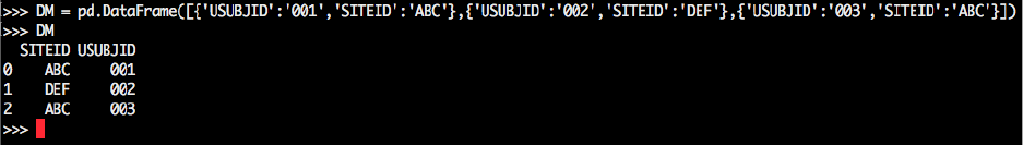
objects from a class. Example 4 below creates a DataFrame object from the DataFrame class.

Example 4

DM =

pd.DataFrame([{'USUBJID':'001','SITEID':'ABC'},{'USUBJID':'002','SITEID':'DEF

'},{'USUBJID':'003','SITEID':'ABC'}])

In this example, we are creating a DataFrame object called DM. We are doing this by calling the

DataFrame constructor prefixed with the "pd" qualifier (from import pandas as pd). The argument of this

constructor is our data – in this case, a list of dictionaries (DMLIST from Example 3 above). Note that

each dictionary has the same keys (USUBJID and SITEID). These keys correspond to the column

headers of our data, and their values to the data values within those columns. Each dictionary represents

a row of the resulting DataFrame. In Figure 5 below, we see that by simply typing the name of the

DataFrame object, we get a two-dimensional representation of it.

Figure 5 - a Pandas DataFrame object

In this case, we formatted our data as a list of dictionaries. Alternatively, we could have formatted it as a

dictionary with list values as in Example 2 above.

DM = pd.DataFrame(DMLIST)

In this case, each key-value pair of the dictionary represent one column of the DataFrame. The key

represents the column header while the list contains all values in order.

SAS gives us several different methods for importing data from several different kinds of sources.

PROCs such as PROC IMPORT allow us to read from Excel or CSV. DDE is an older alternative. The

data step with the IMPORT statement lets us read flat files. The XML engine and XML maps let us use

the LIBNAME statement to read XML. Pandas provides methods for reading Excel, CSV, JSON, and

even SAS files. This means that we can create a DataFrame object from, for example, an Excel file, with

something that looks like a parameterized SAS macro call.

df = pd.read_excel(parameters)

The read_excel method parameters allow you to specify the Excel file as well as the sheets from which

data is to be read, which columns and rows are to be read, where (if any) the header rows are, and how

to process missing values, dates, and thousands separators.

To illustrate Pandas' ability to read Excel as well as other DataFrame functionality throughout the rest of

this paper, we'll use a copy of the NCI controlled terminology spreadsheet illustrated in Figure 6 below.

Figure 6 - SDTM_Terminology_2018-06-29.xlsx

Example 5

sdtmct=pd.read_excel('SDTM_Terminology_2018-06-

29.xlsx',sheetname=1,usecols=[0,1,2,3,4,7],names=['Code','CodeListCode','Exte

nsible','Name','CodeListItem','Decode'],keep_default_na=False)

The first parameter is positional and is the name of the file. This can also contain a path or a URL. The

sheetname parameter defaults to the first tab in the file when not specified. Otherwise it is populated with

an integer as above or a string (name of the tab). Note that while we chose the second tab, we specified

"1" as the value. Almost everything in Python is zero-indexed, which means that to ask for the first of

something, like a sheet in an Excel file, or an element of a list, you specify 0. This parameter can also be

populated with a list of multiple sheets (integers or strings). The usecols parameter specifies a list of

columns to process (again, zero-indexed). In this case, we left out the CDISC synonym and definition.

The names parameter names our columns using a list. Finally, the keep_default_na parameter is a

Boolean (notice the lack of quotation marks). By default, Pandas assumes that certain values (e.g. NA,

N/A, #N/A, and others) are to be interpreted as missing values. Setting this parameter to False turns that

assumption off. Users also have the option of specifying other values which are to be interpreted as

missing through the na_values parameter. Figure 7 shows the result of this method call (first five rows)

using the interactive interpreter.

Figure 7 - SDTM Terminology in a Pandas DataFrame

Before we look at the different ways to work with DataFrames, let's first make two more points. First,

while we have now seen that a DataFrame is a two-dimensional data set-like object, Pandas also has a

one-dimensional object called a Series. A Pandas Series is much like a Python dictionary in that it

contains values, but the values are labeled with an index. When a list of n values is passed to the Series

constructor without an index, then an index with the values 0,1,2,…(n-1) is automatically created.

Otherwise an indexed series can be created either by passing an index parameter to the constructor, or

by passing a dictionary. In Example 6 below, both Series instantiations create a Series object whose

values are the integers 1-5 and whose keys or labels are the letters a-e.

Example 6

ser = pd.Series({'a':1,'b':2,'c':3,'d':4,'e':5})

ser = pd.Series([1,2,3,4,5],index=['a','b','c','d','e'])

The second point that will be helpful to keep in mind going forward is that a DataFrame can be thought of

as a collection of multiple Series all with the same index. This means that unlike a SAS data set, a

DataFrame always has a "special" column called an index, whose purpose is to uniquely identify the rows

of a DataFrame. In SAS, we might know that the observations of a DM data set are uniquely identified by

the USUBJID variable, but to the data set, USUBJID is just another variable whose values we can

capture just like any other column. In a DataFrame, we cannot extract values of the index – we can only

use them to reference rows. Think of an index as a set of labels for rows.

WORKING WITH DATA

Of course SAS programmers spend most of their data step time creating SAS data sets from other SAS

data sets. A simple reading of one data set to create another is accomplished with the SET statement.

Before we see what Python has to offer, let's quickly remind ourselves just how much is packed into this

statement.

Over the years, many of us probably start to take for granted, even become spoiled with what the SET

statement gives us.

data two ; set one ; run ;

In the SAS world, SET is unique in that it operates as both a compile-time and execution-time statement.

At compile time, SET prepares TWO by gathering structural information from ONE. At execution time,

SET begins an iterative cycle by reading one observation from ONE. After all other statements are

executed, SET executes again on the next record from ONE, and so on. Possibly the most challenging

differences for SAS veterans to adjust to when starting with Python, and Pandas in particular, is the fact

that Python has nothing like a SET statement.

df2 = df

The above statement creates a DataFrame called df2 by simply making a copy of the DataFrame df. If df

were an object of any other type (e.g. string, list, etc.) we would say the same thing. No iteration takes

place. This fact will come up again later. For now, let's see how we can simply modify the rows and

columns kept from a source DataFrame to a target.

In SAS, the data step gives us three options each for keeping, dropping, or renaming variables, as well as

filtering observations. Two of these options are data set options on either the DATA or SET statements,

and the third is on a separate statement (i.e. KEEP, DROP, RENAME, WHERE). There are minor

differences in these three options which are not necessary to go through now.

With Pandas, we provide the list of variables to keep in a list.

SAS:

data sdtmct2 ;

set sdtmct ;

keep code codelistitem decode ;

run;

PYTHON:

sdtmct2 = sdtmct[['Code','CodeListItem','Decode']]

Note the two sets of brackets. The outer brackets are part of the Pandas syntax. The inner brackets

denote a list, guaranteeing that sdtmct2 will in fact be a DataFrame object.

Dropping is different, in part, because unlike keeping, dropping requires the use of a method. In addition,

this method not only allows us to drop columns, but it also lets us drop rows, identified by index values.

sdtmct2 = sdtmct.drop(['Code','CodeListItem'], axis=1)

Notice that the drop method has two parameters. The first is a list of the labels to be dropped. The

second, the axis parameter, when set to 1, indicates that the labels are column labels. When set to 0

(default), the labels are index labels.

Renaming is similar to dropping – the use of a method that allows us to rename either column or index

labels. The list from the drop method is replaced with a dictionary where the keys are the names of the

original labels and the values are the new labels. Additionally, instead of an axis parameter, we have

index and columns parameters as a way to indicate what kind of labels are being renamed.

sdtmct2 =

sdtmct.rename(columns={'Code':'SubmissionValueCode','CodeListItem':'Submissio

nValue'})

Filtering data can be accomplished in multiple ways, but the method that most closely resembles the

different options that SAS has is referred to as Boolean indexing. The format is as follows:

df[condition]

The following compares SAS's use of WHERE to Pandas' Boolean indexing for the purpose of extracting

from SDTMCT only those records where the value of CodeListCode is "C141663".

SAS:

data c141663 ; set sdtmct ; if codelistcode eq 'C141663' ; run;

PYTHON:

c141663 = sdtmct[sdtmct['CodeListCode'] == 'C141663']

The SAS data step is reading the data set SDTMCT one record at a time. With the subsetting IF, for any

given record, when the data step reaches this statement, it decides if it should move on with processing

the rest of the statements for that record, or throw out the record and move to the next one. On the other

hand, the expression sdtmct['CodeListCode'] represents a Pandas Series (one of the columns in

the SDTMCT DataFrame). The expression sdtmct['CodeListCode'] == 'C141663' represents a

Boolean Series, one whose values are True and False. The size of this Series matches the number of

rows in SDTMCT (i.e. the size of the index of SDTMCT). In creating c141663, Pandas keeps only the

rows on which the corresponding value of the Boolean Series is True.

We can also use text functions in our criteria. Pandas has several text functions that correspond to string

functions in the general library, some of which correspond to familiar SAS functions.

SAS:

data c141663 ; set sdtmct ; where find(codelistitem,'STR01')>0

PYTHON:

c141663 = sdtmct[sdtmct['CodeListItem'].str.find('STR01')>0]

When creating a new variable, simple calculations are straightforward.

SAS:

data new ; set old ; newcol = oldcol1 + oldcol2 ; run ;

PYTHON:

new = old

new['newcol'] = new['oldcol1'] + new['oldcol2']

This is a good time to remind ourselves of how the processing is taking place. Since SAS is performing

the calculation on one row at a time, it is simply adding two numbers together, and the next time the data

step reaches this statement on the next iteration, it'll perform the same calculation on two different

numbers. In the Python code, the first line creates a new DataFrame called new. The second line is

creating a Series to be added to new, from the sum of two other Series' (new['oldcol1'] and

new['oldcol2']). Two Series are added by adding their corresponding components, resulting in a Series as

large as the largest of the two original Series' (with null values in the positions where the shorter of the

two Series' had no components). The mathematically inclined will recognize this as vector addition.

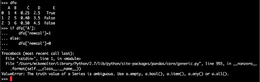
This is important to keep in mind when the logic starts to get more complex. For example, consider a

variable whose values are created conditionally. The SAS data step solution is intuitive.

SAS:

if A then newcol = 1 ; else newcol = 0 ;

We know that Python has conditional logic available …

PYTHON:

if df['A']:

df['newcol'] = 1

else:

df['newcol'] = 0

… but this won't work. Note the message in Figure 8 below.

Figure 8 - Attempt at Python conditional logic on a DataFrame

What does "The truth value of a Series is ambiguous" mean? Keep in mind that while the SAS statement

"if A" is evaluating the value of a single value, df['A'] is a Series that cannot evaluate to a Boolean value.

Pandas does have ways to force Python to evaluate each element of the Series one at a time as SAS

does. Here we'll illustrate a method called list comprehension.

Keep in mind that we're building a Pandas Series. One of the arguments we can feed a Pandas Series

constructor is a list.

mySeries = pd.Series([1,4,9,16])

In this case we explicitly provided each item of the list. List Comprehension allows us to build a list by

providing a function and a set of inputs. An alternate way to construct mySeries is the following:

mySeries = pd.Series(x*x for x in [1,2,3,4])

The other new tool we'll need here is an alternate way of executing conditional logic – the conditional

expression. A conditional expression allows us to condense a traditional conditional construct down into

one statement. For example, the construct here…

if a:

newcol=1

else:

newcol=0

is equivalent to this…

newcol = 1 if a else 0

We can also add conditions

newcol = 1 if a<3 else 2 if a<5 else 3

We can now build a Pandas Series into a DataFrame in which the values are set conditionally by

providing to the Series constructor a list containing a conditional expressional using list comprehension.

df['newcol'] = pd.Series(1 if x else 0 for x in df['A'])

Now, rather than trying to evaluate a Series to a Boolean value, we are iterating through that same Series

(for x in df['A']) and evaluating the logic at each iteration, similar to the data step.

In the example above, we get a glimpse at an ability to iterate through rows of a DataFrame, but the

problem is that the iteration is only through the values of one column, and so we only have access to the

values of that column. What if we want to iterate through a DataFrame and get access to all columns?

For that, we have the iterrows method.

iterrows iterates through each of the rows of a DataFrame and at each iteration returns two items: the

index of the row, and the set of data in that row in the form of a Series. Because two items are returned,

we need two iterating variables.

for index,row in df.iterrows():

<code>

At each iteration (each row of the DataFrame), we can capture the index of the row with a reference to

index. row, on the other hand, is a Series whose data values are the data values in that row of the

DataFrame, and whose index is the set of column headers. Consider once again the controlled

terminology DataFrame found in Figure 7 above.

Figure 9 - print values of selected columns

Here we are iterating through the first five rows (head(n=5)) of the DataFrame df, choosing to print the

value of the index, as well as the values of CodeListItem and Decode.

Going back to creating columns based on conditional logic, iterrows also allows us to base our values

assigned on more than one column. In this case those columns are x and y.

df['newcol'] = pd.Series(1 if (row['x']==1) & (row['y']==1) else 0 for

i,row in df.iterrows())

Pandas has other data manipulation methods as well. DataFrame sorting is one example. As usual,

syntax in SAS translates into the use of standard variable types in Python. In the following example, note

how we specify one of the sorting variables as descending.

SAS:

proc sort data=AE ; by USUBJID descending AETERM ; run ;

PYTHON:

AE.sort_values(by=['USUBJID','AETERM'],ascending=[False,True])

Without the ascending parameter, the default behavior is that Pandas sorts each variable in ascending

order, but if any is to be sorted in descending order, then a Boolean list as long as the BY list must be

provided indicating the sort direction of each BY variable.

Unlike SAS, Python sorts by default, null values of a variable to the bottom, regardless of whether that

variable is sorted in ascending or descending order. Users can change this by setting the na_position

parameter to first. Note that whether first or last, null values will sort to the same place for a descending

sort as they do for an ascending sort.

Pandas also has something like a nodupkey, but it's accomplished with a different method –

drop_duplicates – and has nothing to do with sorting. Without providing any arguments, this method

simply looks for records that are duplicated in all variable values and removes all such records except

one. The subset parameter allows you to specify a subset of variables in which to look for duplicates

(instead of all variables). These are the variables that would be found on your BY statement in a PROC

SORT. Of course, if more than one is needed, they would be provided in a list. In contrast to

NODUPKEY which keeps only the first of multiple records with the same BY values, the keep parameter

allows you to indicate which record to keep. Allowable values are "first" (default), "last", or the Boolean

False, which removes all such records.

SAS:

proc sort nodupkey data=VS out=vs2;

by usubjid vstestcd ;

PYTHON:

vs2=vs.drop_duplicates(subset=['usubjid','vstestcd'])

Merging is also handled in Pandas with a method.

SAS:

data ae2 ;

merge ae(in=inae) suppae(in=insupp where=(qnam eq 'qnam1')) ;

by usubjid ;

if inae ;

PYTHON:

ae2=pd.merge(ae,suppae[suppae['qnam']=='qnam1'],how='left',on='usubjid')

The first positional parameter is the left-most merging DataFrame, and the second is the right-most. Valid

values of the how parameter are left, right, inner, and outer. We can think of these as the SQL join types

– left keeps all records from the left-most DataFrame. Inner would keep only records where the keys

were common to both DataFrames. The SAS equivalent would be to replace if inae ; with if inae and

insupp ;. The on parameter is what SAS users put in their BY statement. When more than one is

necessary, they are provided in a list.

Other parameters include indicator, left_on, right_on, and suffixes. The indicator parameter is Boolean.

When set to True, a new variable, _merge, shows up in your new DataFrame whose values can be

left_only, right_only, or both, to indicate which DataFrames the record came from. When the merge

variable is not the same in the left DataFrame as it is in the right, then we can use left_on and right_on

instead of on to indicate the name of the variable in the first and the name in the second. When non-

merging variables are common to both DataFrames, by default, the resulting DataFrame will contain both

variables, but the one from the left DataFrame will be named with _x on the end, and the one from the

right with _y on the end. Suffixes is a two-tuple with alternate suffixes to be used for this purpose.

PROC TRANSPOSE offers SAS users multiple ways to reshape their data. Pandas offers a light version

of data reshaping through the pivot method.

SAS:

proc transpose data=suppdm out=suppdm2 ;

by usubjid ;

id qnam ;

var qval ;

PYTHON:

suppdm2=suppdm.pivot(index='usubjid',columns='qnam',values='qval')

In both cases, the result has columns named for the values of QNAM, and the contents being the values

of QVAL that correspond to the column and row they are in. The difference is that while values of

USUBJID still define the rows, in the DataFrame, they now define an index, and so USUBJID is not a

column in the SUPPDM2 DataFrame.

In any DataFrame, you can use the reset_index method to turn an index into a DataFrame column.

suppdm2.reset_index()

In addition to the data manipulation we have discussed up to this point, Pandas also has the ability to

generate descriptive statistics like those available in SAS PROCs like MEANS, SUMMARY, and

UNIVARIATE.

SAS:

proc summary data=LB sum mean ;

var lbstresn ;

output out=lbsummary sum= mean= ;

PYTHON:

lbsummary=LB.lbstresn.agg(['sum','mean'])

In this case, we're asking for two statistics of one variable. Note the use of the agg function where we

pass the statistics we want. While the LBSUMMARY resulting data set has a variable for each statistic,

LBSUMMARY is a Series in the Python example, where each entry is indexed by a statistic.

In the case above, we computed the statistics over all records. More typically we want to compute them

once per group of records. In the SAS PROCs, the CLASS statement defines the groups (as well as the

BY statement). In Pandas, we first need to define a new object – a GroupBy object. If LBTESTCD is the

SAS CLASS variable, then we create a GroupBy object as follows.

grpobj=groupby('LBTESTCD')

We can now create summaries by group using the grpobj object.

lbsummary=grpobj.lbstresn.agg(['sum','mean'])

We can also ask for different statistics for different variables.

SAS:

proc summary data=LB sum mean ;

class lbtestcd ;

var lbstresn lbstrnlo ;

output out=lbsummary sum(lbstresn)= mean(lbstrnlo)= ;

PYTHON:

lbsummary=grpobj.agg({'lbstresn':'sum','lbstrnlo':'mean'})

Note the slightly different syntax now that we are summarizing more than one variable. Now we pass a

dictionary into the agg function where the keys are the variables to be summarized, and for each, either a

string or a list (when asking for more than one statistic) that identifies the statistic(s) to compute.

ONE FINAL EXAMPLE - XML

In our final example, we'll see how we can use another third-party package to quickly write XML. In the

meantime, we'll have a chance to make use of groups and see how we can iterate through them to write

XML from each record we read. Before we do that, let's see what our source and our final target look like.

Figure 10 – Source

Figure 10 above shows a portion of a spreadsheet containing a study's controlled terminology. Our task

is to take the two codelists in this spreadsheet and write XML in the format dictated by the ODM/define

standard. For now, we'll just print the generated XML to the command-line screen (as opposed to

creating an XML file). The following illustrates this format with a portion of the AESEV codelist.

<TranslatedText>Grade 1</TranslatedText>

</Decode>

</CodeListItem>

Other CodeListItem elements formatted as above, one for each term

</CodeList>

On the other hand, when no decode exists, as is the case with the Action Taken codelist, we replace the

CodeListItem element with an EnumeratedItem element.

</EnumeratedItem>

Again, the XML above is an abbreviation for space-considerations. The Python code we generate here

will generate complete XML for all codelists read from the source spreadsheet.

Much of this paper has concentrated on the use of the Python Pandas package because it is the premier

package for handling data. These days, however, some SAS programmers are having to think about

creating XML files such as define.xml. Because SAS has the ability to write data to flat files, a

programmer can create the above XML with simple FILE and PUT statements. SAS, however, doesn't

have anything specific to simplify this process, so programmers will have to keep track of when they

generate the start tag of an element and remember to later generate the end tag. They'll have to

generate each "<" and ">", each set of quotation marks around attribute values, and even be sure to know

their logical record length and how to wrap long text that might not fit on one line.

data _null_;

set ct ;

by name ;

if first.name then put "<CodeList Name="+quote(name)

Python's LXML package handles all of those details, leaving it to the programmer just to create objects.

As with Pandas, you will first need to download and install the package, and then import it.

from lxml import etree as et

The syntax here is slightly different from the import statement we saw earlier. We use it here because it

allows us to import a single module (etree) from the LXML package without importing the whole package.

When we think of an XML element, most of us think of text – a start tag, some attributes, some content,

and an end tag. LXML doesn't think of text, it thinks of objects. An Element is an object instantiated from

LXML's Element class by way of a constructor. Remembering that a constructor is a special method, and

that a method looks like a macro call with parameters, it should be no surprise that we can create XML

Elements with parameterized method calls. The first parameter is the name of the element. After that,

we can provide one keyword parameter for each attribute.

Example 7

codelist=et.Element('CodeList',Name='Action Taken with Study Treatment',

DataType='text')

LXML also gives us the SubElement object whose constructor is called like the Element, but the first

argument should be the name of the Element object within which the SubElement is nested.

Example 8

enum=et.SubElement(codelist,'EnumeratedItem',CodedValue='DOSE NOT

CHANGED')

We'll start by using the read_excel Pandas method to read the Excel file illustrated above.

ct=pd.read_excel('SDTM-Metadata-

Worksheet.xlsx',sheetname='Codelists',names=['ID','Name','CodeListCode','Data

Type','Order','Term','TermCode','Decode'],keep_default_na=False)

Note that we are not excluding any columns, but that with the names parameter, we are naming each

column. Now we'll create GroupBy objects – one for each codelist.

ctgp=ct.groupby(['Name','CodeListCode','DataType'])

Earlier we created groups for the purpose of calculating descriptive statistics for each combination of

grouping variable values. Here we're not interested in statistics. However, we can iterate through a

GroupBy object. Each iteration yields 1) the combination of values of the grouping variables, expressed

in a string when there's only one grouping variable, and in a tuple when there are more than one; 2) a

DataFrame specific to that set of grouping variable values.

for n,g in ctgp:

In this case, each iteration corresponds to a unique combination of Name, CodeListCode, and DataType,

expressed in a tuple called n. These values can be captured with n[0] (Name), n[1] (CodeListCode), and

n[2] (DataType). g is a DataFrame whose records are those with values of Name, CodeListCode, and

DataType that match those in n. Looking at the XML we want to generate, now that we are inside a loop

in which each iteration corresponds to a codelist, we want to do three things: create a CodeList Element,

create either a EnumeratedItem or CodeListItem SubElements with any necessary SubElements of those,

and create an Alias Element. The following generates the CodeList Element.

cl=et.Element('CodeList',Name=n[0],DataType=n[2])

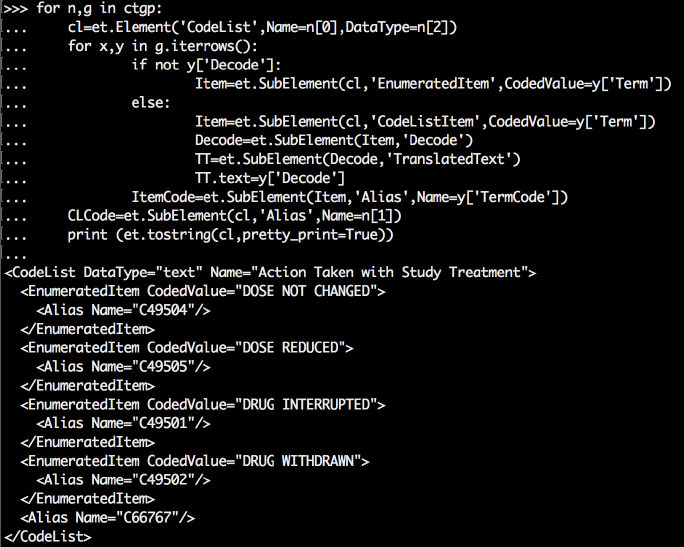
In order now to generate each EnumeratedItem or CodeListItem SubElement, we need to iterate through

the current DataFrame (g). As seen earlier, we can do this with the iterrows method. The following

generates each CodeListItem or EnumeratedItem SubElement.

for x,y in g.iterrows():

if not y['Decode']:

Item=et.SubElement(cl,'EnumeratedItem',CodedValue=y['Term'])

else:

Item=et.SubElement(cl,'CodeListItem',CodedValue=y['Term'])

Decode=et.SubElement(Item,'Decode')

TT=et.SubElement(Decode,'TranslatedText')

TT.text=y['Decode']

ItemCode=et.SubElement(Item,'Alias',Name=y['TermCode'])

Keep in mind that this code is contained within the iteration through groups (for n,g in ctgp), so this is

executing once for each group, so n refers to a specific tuple of values of Name, CodeListCode, and

DataType, and g refers to a specific DataFrame that corresponds to that tuple. With this code, we are

iterating through the records of that specific DataFrame. Remember that with iterrows, we get the index

value (x) and a Series representing the current row (y). We first determine if Decode is populated for this

row (y). Either way we create a SubElement Item. The tag name, attributes and SubElements of Item

depend on whether or not Decode is populated. After this, we generate as a SubElement of Item the

Alias SubElement specific to the item.

Once we are finished iterating through all rows in the current DataFrame (but still iterating with the

GroupBy object), we are then ready to generate the CodeList-specific Alias element and print the current

CodeList.

CLCode=et.SubElement(cl,'Alias',Name=n[1])

print (et.tostring(cl,pretty_print=True))

Figure 11 - code to generate XML and a portion of the resulting output

Since the PRINT statement can print strings but not Element objects, we use the tostring function to

serialize or convert to a string the CodeList element. The pretty_print parameter prints the XML in a

readable fashion.

CONCLUSION

Change can be difficult, and sometimes even downright scary, especially for those of us that have spent

many years not only becoming accustomed to a way of working, but also enjoying it. Ask yourself

though, how did you become a SAS expert. Most likely it didn't happen overnight, so have patience.

Maybe you took advantage of interactive SAS as your playground. Be sure to do the same with Python's

interactive interpreter. Just as with basic data step and PROC processing, get to know the core Python

standard library, as well as the syntax. Make sure to have the thorough Python documentation within

reach. As you get more comfortable, start to branch out into other modules. The industry is changing.

The more we can adapt, the more we can participate in that change.

CONTACT INFORMATION

Your comments and questions are valued and encouraged. Contact the author at:

Mike Molter

919-414-7736

molter.mike@gmail.com

wrightave.com

Any brand and product names are trademarks of their respective companies.