1
A STUDY ON COGNITIVE BIASES IN GAMBLING:
HOT HAND AND GAMBLERS' FALLACY
by
Juemin Xu
Thesis submitted to UCL
for the degree of Doctor of Philosophy in Experimental Psychology
2
I, Juemin Xu, confirm that the work presented in this thesis is my own. Where
information has been derived from other sources, I confirm that this has been
indicated in the thesis.

3
Abstract
People who appear to believe in the hot hand expect winning streaks to continue
whereas those suffering from the gamblers’ fallacy unreasonably expect losing
streaks to reverse. 565,915 sports bets made by 776 online gamblers in 2010 were
used for analysis. People who won were more likely to win again whereas those who
lost were more likely to lose again. However, selection of safer odds after winning
and riskier ones after losing indicates that online sports gamblers expected their luck
to reverse: they suffered from the gamblers’ fallacy. By following in the gamblers’
fallacy, they created their own hot hands. Some gamblers consistently outperformed
their peers. They also consistently made higher profits or lower losses. They show
real expertise. The key of real expertise is the ability to control loss.
4
Publications associated with this thesis
Xu, J., & Harvey, N. (2014). Carry on winning: the gamblers’ fallacy creates hot
hand effects in online gambling. Cognition, 131(2), 173–80.
http://doi.org/10.1016/j.cognition.2014.01.002
Xu, J., & Harvey, N. (2015). Carry on winning: No selection effect. Cognition, 139,
171–173. http://doi.org/10.1016/j.cognition.2015.02.008
Xu, J., & Harvey, N. (2014). The Hot Hand Fallacy and the Gambler’s Fallacy: What
are they and why do people believe in them? In F. Gobet & M. Schiller
(Eds.), Problem Gambling: Cognition, Prevention and Treatment (pp. 61–73).
London: Palgrave Macmillan UK.
http://doi.org/10.1057/9781137272423_3
Xu, J., & Harvey, N. (in press). The economic psychology of gambling. In Ranyard,
R. (Eds.), Economic Psychology: The Science of Economic Mental Life and
Behaviour. Wiley- Blackwell
5
Table of Contents
Chapter 1. Introduction .............................................................................................................. 9
1.1 Classical economic theory about values. .......................................................................... 9
1.2 Behavioural economic theory about values. ................................................................... 10
1.3 Gamblers' theories about uncertainty: the hot hand and gamblers' fallacies. ................. 11
Chapter 2. Gambling games and biases, fallacies, and real skills ............................................ 14
2.1 Lotteries .......................................................................................................................... 16
2.2 Scratch cards ................................................................................................................... 20
2.3 Roulette .......................................................................................................................... 21
2.4 Fruit machines ................................................................................................................ 24
2.5 Sports betting .................................................................................................................. 26
2.6 Card games ..................................................................................................................... 30
2.7 Summary ........................................................................................................................ 32
Chapter 3. Problem gambling .................................................................................................. 34
Chapter 4. The gamblers' fallacy creates the hot-hand effect .................................................. 39
4.1 Data set ........................................................................................................................... 39
4.2 Methodology and results ................................................................................................ 41
4.3 Do gamblers with long winning streaks have higher payoffs? No. ................................ 47
4.4 The effects of winning and losing streaks on level of odds selected. ............................ 48
4.5 The effects of winning and losing streaks on stake size ................................................. 51
4.5 Hot hands exist because of a belief in the gamblers’ fallacy ........................................ 53
6
4.6 Gamblers became safer or riskier after winning or losing streaks, not the other
way round. ............................................................................................................................ 54
Chapter 5. A roulette experiment ............................................................................................. 60
5.1 Methodology .................................................................................................................. 60
5.2 Results ............................................................................................................................ 62
5.4 Discussion ...................................................................................................................... 67
Chapter 6. Real expertise in gambling .................................................................................... 69
6.1 Is there real expertise? Yes. ............................................................................................ 70
6.2 What is real expertise? The ability to control loss. ........................................................ 78
Chapter 7 Discussion and summary ......................................................................................... 84
7.1 Evidence for the hot hand but not for the gamblers’ fallacy. ......................................... 84
7.2 Gamblers behave differently in roulette and in sports gambling. .................................. 85
7.3 There is real expertise in sports gambling: it is loss control. ......................................... 85
References ................................................................................................................................ 87
7
List of Figures
Figure 1. Probability of winning after obtaining winning streaks of different lengths
(o) and after not obtaining winning streaks of those lengths (Δ). .............................. 42
Figure 2. Probability of winning after obtaining losing streaks of different lengths (o)
and after not obtaining losing streaks of those lengths (Δ). ....................................... 45
Figure 3a. Mean preferred odds after winning (o) and losing (Δ) streaks of different
lengths. ....................................................................................................................... 49
Figure 3b. Median preferred odds after winning (o) and losing (Δ) streaks of
different lengths. ........................................................................................................ 50
Figure 4. Median stake size after winning (o) and losing (Δ) streaks of different
lengths. ....................................................................................................................... 52
Figure 5. Mean odds plotted against streak length. The continuous line with the “o”
symbol shows data for consecutive wins and the dotted line with the “▢” symbol
shows data for consecutive losses. ............................................................................. 57
Figure 6. Median odds change in always win (o) and always lose (Δ) rounds. ......... 63
Figure 7. Median stake change in always win (o) and always lose (Δ) rounds. ........ 65
8
List of Tables
Table 1. Common forms of gambling ........................................................................ 15
Table 2. Sample characteristics for sports bets placed in each of three currencies for
the year 2010. ............................................................................................... 40
Table 3. Regressions for length of streaks predicting the probability of winning. .... 47
Table 4. Regression for length of streaks predicting the odds. .................................. 64
Table 5. Regression for length of streaks predicting the stake. ................................. 66
Table 6. Binary regression of winning and losing amounts predicting change of
chosen slot. ................................................................................................... 67
Table 7. Monthly median and mean returns in horse racing and football. ................ 71
Table 8. The performance ranking in horse racing in each month was correlated with
the rankings in the other months. ................................................................. 72
Table 9. Positive returns in horse racing in one month were correlated with returns in
other months................................................................................................. 75
Table 10. Performance ranking in football in each month was correlated with the
rankings in the other months. ....................................................................... 77
Table 11. Positive returns in football in one month was correlated with returns in
other months................................................................................................. 78
Table 12. Profitable gamblers were less likely to chase loss. .................................... 81
9
Chapter 1. Introduction
Gambling, being a game of money, gives us a peep into the psychology of
value. Gambling has a long history. It typically involves winning or losing money
with uncertainties. It is one of the earliest behaviours studied in scientific research
into probability (Bernoulli, 1738/1954).
1.1 Classical economic theory about values.
Economics is a science about values (e.g. money, probability). One common
value is money. In microeconomics, the value of money is ultimately defined by
utilities. Utility is subjective. This means that microeconomics is usually implicitly
based on psychology. Classical economics assumes people want to maximize their
utility and their own utility only, and that they know how to maximize this utility
with minimum cost. Through self-interest, people can trade with each other to
maximize their own utility. Their preferences are stable: in other words, they have a
stable utility function. Their behaviours are consistent with their utility functions. A
large group of people or one person over time, given enough resources to gather
information, should demonstrate, or at least approach, rational decision making.
People are assumed to prefer more money than less money. Money has
diminishing marginal return of utility: all else being equal, every additional unit of
money brings less pleasure. This view is partially derived from the law of
diminishing marginal returns (Smith, 1776). For example, when a person is thirsty,
drinking the first cup of water quenches the thirst most; drinking the second cup of
water may still be nice but may not be as wonderful; a third cup may be OK;
drinking a fourth or fifth cup will eventually bring misery. Many other products may
10
not have such a steep decrease of marginal utility but the pleasure of owning one
more unit of the same product almost always decreases after more units have been
acquired. Money provides the payment method for products and has a similar
diminishing marginal utility.
1.2 Behavioural economic theory about values.
When an economic decision involves uncertainty, the option with the highest
expected value has been assumed to be the preferred choice. If the same decision is
repeated many times, the mean value will approach the expected value. However,
questions have been raised by economists about the validity of using expected value
as the only indicator of preferred choice. In many situations, people consistently
prefer a lower expected value. For example, in insurance, the very fact that the
organizers make profit from the business is a sign that the expected value of the
potential loss is lower than the insurance premium; and in lotteries, the expected
value of the jackpot is almost always lower than the lottery ticket. So why do the
buyers accept a loss? This is likely to be because they have a risk preference that is
different from what is assumed by expected value maximization. Specifically, some
people may prefer to lose a small amount of money for sure rather than a large
amount with small probability. A person who prefers a sure option over a risky
option that has an equal or greater expected value is, for that particular choice at least,
risk averse. Conversely, a person who prefers a risky option over a sure option that
has an equal or greater expected value is risk seeking.
Prospect theory says people value same amount of loss more than same
amount of gain (Kahneman and Tversky, 1979). What's more, people tend to have
different risk preferences for different probabilities (Tversky and Kahneman, 1992;
11
Tversky and Fox, 1995) and for different amounts of money (Markowitz, 1952;
Levey, 1994). Generally speaking, when the decision is about receiving money,
people are risk seeking when probabilities of the largest possible outcome are low
but risk averse when they are high. Thus, Tversky and Fox (1992) re-analysed
Tversky and Kahneman’s (1992) data to show that the certainty equivalent of 5%
chance of receiving $100 was a gain of $14 (risk seeking) but that the certainty
equivalent of a 95% chance of receiving $100 was a gain of $78 (risk aversion). This
pattern was reversed when the decision was about losing money: the certainty
equivalent of a 5% chance of losing $100 was a loss of $8 (risk aversion) whereas
the certainty equivalent of a 95% chance of losing $100 was a loss of $84 (risk
seeking). This fourfold pattern of risk taking is overlaid by effects of the amount of
money to be gained or lost. Thus the risk aversion with gains increases with the size
of the stake (Binswanger, 1981; Levy, 1994).
When people make a decision that involves both a gain and a loss, they tend
to display loss aversion. For example, people who are offered a bet, which has 50%
chance of winning £10 and 50% chance of losing £10, will often refuse it
(Kahneman and Tversky, 1979). This implies that they anticipate that their pain from
losing £10 will be greater than the pleasure from winning £10. Hence, for people to
take the risk of losing £10, their potential gain needs to be bigger than that amount.
In this chapter, I will discuss the economic psychology of gambling in terms of these
three concepts: risk aversion, risk seeking, and loss aversion.
1.3 Gamblers' theories about uncertainty: the hot hand and gamblers' fallacies.
To gamblers, uncertainty is intertwined with luck. When luck is with you,
you can win in spite of low chance of winning; when luck is not with you, you could
12
fail even with a good chance of winning. The hot-hand fallacy and gamblers’ fallacy
are assumed to be common among gamblers because it is thought that they have a
strong tendency to believe that outcomes for future bets are predictable from those of
previous ones. In chapter 4, a mechanism of the gamblers' fallacy creating the hot-
hand effect will be revealed.
Belief in a hot-hand is “If you have been winning, you are more likely to win
again.” The term “hot hand” was initially used in basketball to describe a basketball
player who had been very successful in scoring over a short period. It was believed
that such a player had a “hot hand” and that other players should pass the ball to him
to score more. This term is now used more generally to describe someone who is
winning persistently and can be regarded as “in luck”. In gambling scenarios, a
player with a genuine hot hand should keep betting and bet more.
There have been extensive discussions about the existence of the hot hand
effect. Some researchers have failed to find any evidence of such an effect (Gilovich,
Vallone and Tversky, 1985; Wardrop, 1999; Koehler and Conley, 2003; Larkey,
Smith & Kadane, 1989).
Others claim there is evidence of the hot hand effect in games that require
considerable physical skill, such as golf, darts, and basketball (Gilden and Wilson,
1995; Arkes, 2011; Yaari and Eisenmann, 2011).
People gambling on sports outcomes may continue to do so after winning
because they believe they have a hot hand. Such a belief may be a fallacy. It is,
however, possible that their belief is reasonable. For example, on some occasions,
they may realize that their betting strategy is producing profits and that it would be
sensible to continue with it. Alternatively, a hot hand could arise from some change
in their betting strategy. For example, after winning, they may modify their bets in
13
some way to increase their chances of winning again.
The gamblers’ fallacy is “If you have been losing, you are more likely to win
in future.” People gambling on sports outcomes may continue to do so after losing
because they believe in the gamblers’ fallacy. This is the erroneous belief that
deviations from initial expectations are corrected even when outcomes are produced
by independent random processes. Thus, people’s initial expectations that, in the
long run, tosses of a fair coin will result in a 50:50 chance of heads and tails are
associated with a belief that deviations from that ratio will be corrected. Hence, if
five tosses of a fair coin have produced a sequence of five heads, the chance of tails
on the next toss will be judged to be larger than 50%. This is because the coin “ought
to” have a 50:50 chance of heads and tails in the long run and, as a result, more tails
are “needed” to correct the deviation from that ratio produced by the first five tosses.
There is a conflict between belief in a hot hand and the gambler’s fallacy.
Betting strategies are often based on the previous betting results (Oskarsson, Van
Boven, McClelland, and Reid, 2009). The strategies based on a belief in a hot hand
and gamblers’ fallacy may conflict. For example, when trying to decide what odds to
select in the next round, a belief in the gamblers’ fallacy would result in betting on
higher odds and with more money after losing than after winning. A believer in the
hot hand would do the opposite. In this way, the hot hand and the gamblers' fallacy
give contradictory predictions. They cannot both be true. It is worth investigating
which strategy the gamblers use.
There are many biases, fallacies, and even real skills in gambling, which will
be described in the next chapter.
14
Chapter 2. Gambling games and biases, fallacies, and real skills
In what follows, I discuss the six popular forms of gambling listed in Table 1
and indicate how they illustrate the way that people reason about money and
probability. After that, I discuss the economic, psychological and neurological roots
of problem gambling in chapter 3.

15
Table 1. Common forms of gambling
Game
Characteristics
Prevalence as a percentage
of all UK adults (Wardle,
Moody, Spence, Orford,
Volberg, Jotangia, 2011)
Biases, fallacies, and
other reasons to gamble
Lottery
Low frequency,
fixed odds,
pure chance.
National lottery 59%;
Other lotteries 25%.
Overestimation of low
odds; The availability
heuristic; Entrapment;
The endowment effect;
The representativeness
heuristic;
Illusions of control;
The gamblers' fallacy;
The hot hand effect;
Superstitious
behaviour;
The near miss effect;
Mental accounting;
Loss chasing;
High testosterone
levels; Abnormal levels
of neurotransmitters;
Abnormal brain
activity;
Card counting (a real
skill).
Scratch
cards
High frequency,
fixed odds,
pure chance.
24%
Roulette
High frequency,
fixed odds,
pure chance.
In a casino 5%;
Online games that include
roulette13%.
Fruit
machine
s
High frequency,
fixed odds,
pure chance.
18%
Sports
betting
High frequency,
flexible odds,
may involve real
skills.
Horse racing 16%;
Football 4%;
Dog racing 4%;
Other sports events 9%.
Card
games
High frequency,
flexible odds,
may involve real
skills.
Poker (pub or club) 2%;
Casino card games 5%;
Online games that include
card games 13%.
16
2.1 Lotteries
A lottery is a common form of gambling. There are at least 180 lotteries
worldwide and the total size of lottery industry is estimated to be $284 billion
according to La Fleur's 2015 World Lottery Almanac (Markel, La Fleur and La Fleur,
2015). In the UK, 59% of adults purchased National Lottery tickets in 2009 (Wardle
et al, 2011). Typically, a lottery gambler chooses a series of numbers and pays a
small fixed price for the lottery ticket. The winning numbers are announced
periodically, usually a couple of times a week. The chance of winning the jackpot is
typically extremely low.
As an example, consider Lotto, one of the games offered by the UK National
Lottery. With a £2 lottery ticket, the buyer chooses six numbers from a range
between one and 59 or, alternatively, they take the Lucky Dip option and a machine
picks the six numbers for them. There are two draws every week, one on Wednesday
and one on Saturday. To win the jackpot, all six numbers on the lottery ticket must
match the six winning numbers.
There are 45,057,474 combinations of six winning numbers. In 2015, the
jackpot size fluctuated from £886,754 to £43 million (Camelot, 2015).
Apart from the jackpot, there are smaller prizes for people with tickets that
have fewer than six numbers that match those selected. For those with five matching
numbers, the prize is estimated to be £1000. However, if the number that fails to
match one of the six that are selected does match the number on the bonus ball, then
winnings can rise to around £50,000. There is also £100 for those with four matching
numbers, £25 for those with tickets with three, and a free Lotto ticket for those with
two. There is also a complimentary Millionaire Raffle included with each £2 ticket.

17
A particular combination of colour and an eight-digit number wins a £1 million
prize; there are also twenty £20,000 prizes in every draw.
Every time a person buys a £2 lottery ticket, they are expected to lose half of
the money. The chance of winning any prize is 1 out of 9.3. Clearly, buying a lottery
ticket is not an efficient way to make money. Other lotteries in the world are also
fairly similar to the lottery games organised the UK National Lottery and have
similar returns. For example, the expected return from participating in Powerball in
the USA is about $0.90 for a $2 ticket and 1 in 24.87 buyers win a prize. It is clear
from these odds that buying lottery tickets does not earn money. So why do people
do it?
Lottery buyers may miscalculate and believe they can make money.
According to prospect theory, people tend to overestimate low odds of winning
(Tversky and Kahneman, 1992). Because the extremely low odds of winning the
jackpot are far lower than what people experience in everyday life, they may not be
able to estimate just how tiny they actually are.
Our understanding of the environment comes from experience. According to
Decision by sampling theory (Stewart, Chater and Brown, 2006), each of our
experiences is saved as a sample in memory. It is extremely rare to encounter an
event with a miniscule chance of occurring. Therefore it is unlikely that the chance
of such an event is represented in memory. As a result, it is really difficult to imagine
a chance of this sort. Consequently, people are likely to use a small chance that they
have retained in memory as a substitute for a minuscule chance that they have never
encountered before. The small chance they think of could be a lot bigger than the
miniscule chance.
18
Another way that people may overestimate the chance of winning a lottery is
by using the availability heuristic (Tversky and Kahneman, 1973). In other words,
they may estimate the probability of winning by recalling how many lottery winners
they have heard of. For example, their attention may have been drawn to news
coverage of a number of highly impressive jackpot wins and, as a result, they over-
estimate their chances of winning (Bordalo, Gennaioli and Shleifer, 2010). The
bigger the jackpot, the more jackpot winners are reported and the more people buy
lottery tickets (Cook and Clotfelter, 1991; Matheson and Grote, 2004). When an
event is sufficiently important (for example, involving a life changing amount of
money), people may neglect the actual probability and decide that the event’s
occurrence is all or none (Loewenstein, Weber, Hsee, and Welch, 2001;
Rottenstreich and Hsee, 2001).
People may play a lottery together with friends as a social activity. They may
also buy lottery ticket to experience excitement. In other words, they buy a short
"dream" of winning the jackpot and may be "entrapped" by the thought that, if they
stop buying tickets, they will miss the jackpot (Beckert and Lutter, 2013; Binde,
2013; Forrest, Simmons and Chesters, 2002). These motivations all focus on what
winning lottery would be like rather than on the expected value of buying a ticket.
After people have concluded that the lottery is a good way of making money,
they invent methods to increase their chances of winning. The randomness of the
lottery is closely monitored by its organisers, the regulation bodies, lottery machine
engineers, independent researchers, and millions of buyers (Camelot, 2016a;
Gambling Commission, 2012; Konstantinou, Liagkou, Spirakis, Stamatiou and Yung,
2005). However, this does not stop people trying to increase their chances of
19
winning. Searching online using keywords such as "predict lottery" and "lottery tips"
produces numerous suggestions for doing so.
These tips for increasing the chances of winning can often be traced back to
well-known cognitive biases. For example, people using the representativeness
heuristic are likely to expect that the winning numbers should look random. As a
result, they avoid numbers that do not look random enough, such as those with
regular intervals or those that do not distribute sparsely across the whole range of
possible numbers (Holtgraves and Skeel, 1992; Hardoon, Barboushkin, Derevensky
and Gupta, 2001). Also, given their susceptibility to the illusion of control (Langer,
1975; Rudski, 2004), people overestimate their ability of choosing winning numbers.
This is likely to be why they prefer numbers that they have chosen themselves (Wohl
and Enzle, 2002). In addition, there is evidence that people are affected by the
gamblers' fallacy. If certain numbers have recently appeared among the winning
ones, people tend not to bet on them whereas, if particular numbers have not
appeared for a long time, they are more likely to bet on them (Clotfelter and Cook,
1991; Terrell, 1994). People may also be affected by a belief that certain numbers are
lucky. As a result, they make efforts to find out which those lucky numbers are by
visiting temples, observing candle tears, examining incense ashes, and so on
(Ariyabuddhiphongs and Chanchalermporn, 2007). People also display the
endowment effect: they value things they own more than the same things if they do
not own (Kahneman, Knetsch and Thaler, 1991). Cognitive biases of the sort
outlined above have also been exploited within the commercial advertising to sell
lottery tickets (McMullan and Miller, 2009). I have recently come across a hand-
written lottery advertisement on the Chinese website, weibo.com. It says "You
already have 10 million Yuan in your bank account. You have only forgotten the
20
password. It costs 2 Yuan to try out a password. Once you have got the right
password, the money is yours. No rush, don't give up. Your heart is here, your dream
is here. Chinese Lottery." This is a good example of the endowment effect.
These sorts of effects may have consequences beyond financial loss. People
who believe that there are ways of winning the lottery and who act in ways
consistent with those beliefs exhibit the sort of flawed judgement and decision
making that can make them prone to problem gambling.
Does winning the jackpot make people happy? From the huge smiles of the
lottery winners, it is obvious that jackpots bring instant ecstasy. Surprisingly,
however, Brickman, Coates and Janoff-Bulman (1978) found that winning a jackpot
does not produce longer term happiness. They attributed this to the stresses
associated with the large changes in life style and the increased responsibilities
arising from such a win. Consistent with this, winning a relatively small amount, e.g.
£5000, which is insufficient to lead to a change in life style or to increase financial
responsibilities does make people happier (Gardner and Oswald, 2007).
2.2 Scratch cards
Twenty-four percent of all the adults in UK played scratch cards in 2010
(Wardle et al, 2011). A scratch card is typically a paper card coated with a layer of
black silver ink. The ink can be scratched off to reveal winning numbers or symbols
underneath. The UK National Lottery sells them for prices ranging between £1 and
£10. There can be more than one game on one card. Each game has its own rules.
For example, one scratch card sold for £10 is called £4 Million Blue. It is a blue card
claiming to have four top prizes of £4 million each. It contains a number of games.
The first one requires a purchaser to find the UK National Lottery logo to win.
21
Suppose that, after the ink has been scratched off, a bank symbol showing £4 million,
a vault symbol showing £5000, a suitcase symbol showing £50, and a cash symbol
showing £10,000 are revealed. In this case, the purchaser does not win. If the Lotto
symbol appears, the purchaser wins 4 million. Other games are similar, though some
top prizes are smaller than £4 million.
The odds of winning after purchasing a scratch card range from a 1 in
4,347,890 chance of winning £4 million to a 1 in 6 chance of winning £10 (Camelot,
2016b). The expected return at the start of the game is £7. As the cost of the card is
£10, the buyer is expected to lose £3 for every purchase.
The main difference between scratch cards and the lottery is that results from
scratch cards are instant. In fact, one of the scratch cards sold by the UK National
Lottery is called Instant Lotto. Because the result of the gamble is revealed within
seconds after buying the scratch card, people can quickly buy another one if they so
wish. This makes it easier for people to become addicted to purchasing scratch cards:
if they win, they may feel lucky and buy another scratch card; if they lose, they may
display the gamblers' fallacy and decide to have another try (Griffiths, 2000).
Another difference is that, after the initial print run of the scratch cards, the winning
chance changes after winning cards have been claimed.
People display "near miss" effects with scratch cards, which we will discuss
in detail in section 2.4 in the context of fruit machines.
2.3 Roulette
In 2010, 9% of the adult population in UK played casino games, including
roulette, whereas 13% gambled online, again including roulette (Wardle et al, 2011).
22
Roulette requires no skill. It is a game of pure chance. The odds are completely clear
and transparent. The rules are simple. There are 37 slots on the European roulette
wheel (38 on the American one). Numbers range from 0 to 36 (with an extra 00 slot
on the American roulette wheel). Half are red, half are black, and 0 and 00 are green.
Gamblers can choose to bet on a single slot or a selection of slots. For example, they
could select even or odd, red or black, the first 12 numbers, the second 12 numbers,
the third 12 numbers, and so on. The pay-out for a single number is 35 to 1, the pay-
out for even or odd and for red or black is 1 to1, and the pay-out for any selection of
12 numbers is 2 to 1. It is easy to see that the odds against winning for a single
number are 36 to 1 (37 to 1 on the American roulette). The return is the profit a
gambler can expect based on the pay-out. The expected return divides the expected
profit by the investment (Flood, 2017). In the case of roulette, the expected return is
the expected pay-out divided by the wager. The expected return in European roulette
is -1/37 for a single number. For other choices, when the pay-out decreases, the
chances of winning increases correspondingly and so the expected return is the same.
For American roulette, similar principles hold but the expected return is -2/38.
The result of the roulette game is available immediately and gamblers can
play again immediately. Because of this, roulette is a good game to discuss loss
chasing. Loss chasing is characteristic of problem gamblers according to Diagnostic
and Statistical Manual of Mental Disorders, 5th edition (DSM-5) (American
Psychiatric Association, 2014). To normal people, if something brings pleasure, they
do more of it; if something brings pain, they do less of it. Losing money is certainly
painful, or least unpleasant. However, it is quite common for gamblers to gamble
more after losing. They chase their loss in an attempt to get their money back.
Gamblers may have a mental account for each session of gambling (Shefrin and
23
Statman, 1985; Thaler and Johnson, 1990). When they are still gambling, the book is
not yet closed. They have not "lost". When gamblers are losing, they would face a
sure loss if they stopped. However, if they continued to gamble, then their final loss
would not yet be confirmed. In other words, they would be facing an uncertain loss
with some possibility of winning back their money.
According to prospect theory, people tend to be risk seeking when choosing
between a large uncertain loss and a smaller sure loss (Kahneman and Tversky,
1979). For example, the vast majority of people prefer an 80% chance of losing 4000
Israeli Shekels to a sure loss of 3000 Shekels (the median family net income).
Furthermore, once they have lost, they somehow believe that their luck will turn;
they cannot always lose; god must be fair. This is the gamblers' fallacy (Croson and
Sundali, 2005). It leads to loss chasing. In order to catch the anticipated forthcoming
good luck, they must continue gambling. It is possible that, by chasing loss,
gamblers make themselves even more likely to lose. Because they think good luck is
about to arrive after a losing streak, they bet on longer odds to win more money back
and to make most out of the forthcoming good luck. However, longer odds, by their
very nature, mean a higher likelihood of loss. So, unfortunately, gamblers bring back
luck upon themselves by believing that good luck is on its way.
There is even a betting strategy based on the gamblers' fallacy. It's called the
martingale (Snell, 1982; Wagenaar, 1988). It claims to guarantee winning in a
gambling session. The original model of the martingale strategy is based on coin flip
but it "works" in roulette as well. Here is an example of what it involves. Your first
stake is £1 on red. If you win, you stop. If you lose £1, you double your next stake to
£2. If you win, you stop. If you lose again, you double your third stake again to £4. If
you win, you stop. If you lose again, you double the stake again to £8. And so on.
24
Now suppose that you have lost three times but, finally, won. You will get £8 - £4-
£2 - £1 = £1, if you bet on the 1:1 pay-out choice. (In fact, the expected value on a
£1 stake is 36/37 or 36/38). You could win more if you bet on other higher pay-out
slots. This sounds like a brilliant strategy because, no matter how many times you
lose, you can always win in the end.
Unfortunately, there is a catch: it is quite possible that a gambler will run out
of funds after a losing streak. The roulette ball does not remember its history. Thus,
that gambler is no more likely to win after losing streak than in any other round. Of
course, for gamblers who have an infinite amount of money, the martingale is a
reasonable strategy. Most of them, however, do not have an infinite amount of
money to continue the game. In a limited number of rounds, the return could deviate
far away from the expected value. With erroneous beliefs, people can be trapped in
loss chasing and become problem gamblers. Though it is difficult to ascertain how
many people use the martingale strategy, there are written records of it covering
hundreds of years at least (Scarne, 1961). One vivid story is by Casanova
(1822/2013): "Playing the martingale, continually doubling my stake, I won every
day during the rest of the carnival. I was fortunate enough never to lose the sixth
card … I still played the martingale, but with such bad luck that I was soon left
without a sequin".
2.4 Fruit machines
In 2010, 18% of all adults in UK played fruit machines in 2010 (Wardle et al,
2011). Fruit machines are said to be most addictive form of gambling because of
their highly stimulating sounds and colours. According to Turner and Horbay (2004),
25
it takes just over a year to become addicted to them, whereas it takes over three years
with traditional table games, such as roulette.
Fruit machines, like scratch cards, represent a form of gambling that has no
specific odds of winning. They look like vending machines and work like them.
Typically, they have three to five reels on which pictures are depicted. The player
inserts a coin and then pulls down a handle or presses a button. The reels spin. When
they stop, the combination of pictures forms a certain pattern. If the combination
comprises three pictures that are the same (or some other designated pattern), a
reward is given. The most common winning combination is 777. The odds of
winning on fruit machines are unknown. The fact that it is a game of pure chance
and that the owners of the machines make money indicates that luck is unlikely on
the gamblers' side.
One of the main phenomena identified in studies of fruit machine gambling is
the effect of a near miss. This is a losing pattern that is very similar to a winning one.
For example, the three reels may stop at 776, a combination very similar to the
winning 777. In fact, this sort of result should really be labelled a near win.
Occurrence of a near miss makes the gamblers feel that luck is with them and that
success is on its way. As a result, near miss experiences tend to encourage more
gambling (Reid, 1986; Griffiths, 1991).
In natural environments to which we are adapted by evolution, a near miss
may indeed be close to win. For example, almost catching prey clearly indicates that
prey is nearby and your skill levels are probably adequate to make a kill. In these
circumstances, it makes sense to continue to hunt. However, in artificial
environments, this link may no longer hold. A 776 in fruit machine does not indicate
26
that the result of the next spin is likely to be 777. A piece of valid natural reasoning
has been hijacked. In fact, with functional magnetic resonance imaging, it has been
found that the part of brain that responds to real winning also responds to near miss
(Clark, Lawrence, Astley-Jones and Gray, 2009). This supports the notion that a near
miss is a loss that is either mistaken for gain or that is taken to indicate an
expectation that persistence will produce a gain. Any confusion between losses and
gains could lead to problem gambling. This is because near misses that are registered
in the brain as gains will result in gamblers receiving positive reinforcement even
when they are losing money. As a result, they would encourage people to gamble
more.
2.5 Sports betting
In 2010, 16% of adults in the UK gambled on horse races, 4% on football
matches, 4% on dog races, and 9% played on other types of sports betting (Wardle et
al, 2011).
In sports betting, people bet money on the outcome of sports events. Here we
include non-human sports events, such as horse racing and dog racing, as well as
human sports events like football, tennis, and so on. This is because the format of the
gambling is similar and gambling houses include betting on non-human sports as
sports betting. Gamblers can bet against the bookmaker or against each other in a
betting exchange. Traditionally, the bookmaker sets the odds, the gamblers bet that a
certain event will occur (back) and the bookmaker bets that it will not (lay). This
traditional form of gambling can be done in gambling outlets or on the bookmakers’
websites.
27
Betting exchange typically takes place on bookmakers’ websites. Gamblers
bet against each other. They can offer to "back" a certain event, or to "lay" a certain
event. Their counterparts can see the offers and choose the best odds. Bookmakers in
this scenario work as risk-free exchange houses and do not get involved in the price
setting of the odds. They display matches and settle the odds for a small percentage
of commission. In both betting against the bookmaker and in betting exchange, many
different bets can often be made on one event. For example, for a single football
match, there can be bets on the total score, the first half score, the second half score,
the first team or player to score a goal, the number of goals over or under a certain
number, and so on. The range of odds can be wide. For example, they can range
from 4:3 for "both teams to score" to 150:1 for "over 9.5 goals". Hence, gamblers
can choose from many different types of bet and can select from a wide range of
different risk levels.
Gamblers who back a certain event can choose to hedge their position by
laying that event in the exchange. This could reduce or eliminate the risk they are
exposed to. For example, a gambler who has placed £10 on odds of 150:1 for "over
9.5 goals" may find that the prevailing odds for the same event become 50:1 after
four goals in the first half. He may decide to lay 50:1 "over 9.5 goals" for £20
backer's stake. In other words, he now believes the final result will not exceed 9.5
goals and so he accepts a £20 stake from another gambler who believes the final
result will exceed 9.5 goals. If the final score is over 9.5, he will win £1490 from his
first bet, lose £980 from his second bet, and so win £510 overall (minus commission).
If the final score is under 9.5, he will lose the £10 stake in the first bet, win the £20
stake in the second bet, and so win £10 overall (minus commission). At half time,

28
this gambler can guarantee making profit no matter what the final score is. Such
hedging is a real skill that gamblers can learn.
Among gamblers, it is widely believed that there is useful knowledge to be
learned about different sports. There are books, columns and websites that provide
tips for betting. Betting companies also sell past records to people who want to carry
out analyses. However, researchers have not found much evidence of expertise
(Ladouceur, Giroux and Jacques 1998; Cantinotti, Ladouceur and Jacques, 2004).
Ladouceur, Giroux and Jacques (1998) found that experts won more times than
randomly selected betters but did not win any more money. Experts were just being
cautious and chose safe bets, but they still lost money overall. If this is to be called
an expert strategy, then so should the strategy of not gambling at all as this would
have a non-negative return of zero.
Gamblers feel empowered by knowing the past records of sports teams and
the latest updates. Their confidence level is increased, but their performance level is
not (Cantinotti, Ladouceur and Jacques, 2004). Research has shown that experienced
betters make more accurate judgments in complicated tasks, such as the final score
of a game and the ball control time by each team in a game in football. However,
they do not perform any better in simple tasks, such as predicting which teams went
through to t he next round in the World Cup 2006 (Andersson, Memmert and
Popowicz, 2009). It is not clear whether experienced betters can make profits or not.
It is not impossible that some gamblers have inside information (Crafts, 1985).
Superstition is common in sports gambling. Windross (2003) found that a
majority of people betting on horseracing believed in luck and they practiced
superstitious ceremonies to create good luck. The superstitious behaviours include
29
choosing a lucky number or lucky colour, finding a lucky letter combination in horse
names, combining the numbers of the two previous winning horses, and so on.
Gamblers believe luck can be observed and manipulated. Superstitious rituals are the
methods that are used to obtain good luck. Some rituals can appear bizarre and
dangerous. For example, in South East Asia, some people run in front of trucks on
highways to read their number plates. The number plate gives clues of the lucky
number. The closer the gambler runs to the truck, the luckier the number.
When people have no control over uncertainty, they may turn to superstition
in an attempt to feel that they are still in charge. The hot hand fallacy represents one
such illusion of control. This is the belief that winning brings forth more winning. In
skill-based games, people may believe that winning is a signal that a period of
especially good performance has started and that it will continue. As a result, a streak
of winning indicates that the streak will continue. Ayton and Fischer (2004)
discovered that people who were told that a run of the same outcome was the result
of random process predicted the trend would reverse whereas those who were told
that the same sequence was the result of an algorithm predicted that it would
continue. Fischer and Savranevski (2015) obtained a similar result.
This begs an obvious question: do gamblers believe that sports-betting is
skill-based or not? If they believe that it is their skills that give them an edge, they
should predict they are more likely to win after winning and therefore become more
risk seeking. Xu and Harvey (2014) discovered the opposite: in sports gambling,
gamblers predicted the trend in their betting performance would reverse. They were
more risk averse after winning and more risk seeking after losing. They chose safer
odds after winning and riskier odds after losing. Interestingly, this actually produced
a hot hand effect because safer odds are more likely to produce a win and risky odds
30
are more likely to produce a loss. However, safer odds do not have high payoffs.
Hence, gamblers who have experienced a winning streak may feel that their
gambling performance has improved even though they have not actually made more
profits. This echoes the observation by Ladouceur, Paquet and Dubé (1996) that
experts did not make more money in spite of higher probability of winning. They
might become experts simply by winning more times rather than winning more
money. They can be expert and problem gamblers at the same time. However, good
moods resulting from previous wins may lead to risk aversion in future bets (Isen &
Patrick, 1984). When people are in a good mood, they may choose safer bets to
maintain that mood by avoiding losses. This is an alternative explanation to Xu and
Harvey (2014). This could also create hot hand phenomenon even if the estimate of
the risk level of the future bets remains unchanged.
2.6 Card games
Wardle et al (2011) reports that, in 2010, 2% of adults in the UK played
poker in a pub or club, 5% went to a casino to gamble on games (including poker
and blackjack), and 13% played online games (including poker and blackjack).
There are many different kinds of card games. Some of them, such as blackjack and
poker, have both elements of luck and of real expertise. In blackjack, which is also
called twenty-one, the players take cards in rounds and the one who wins is the
person who reaches 21 points or who is the closest to 21 without exceeding that
number of points. It is played between the dealer of the house and one or more
gamblers. If players can remember the cards that have already appeared in the game,
they will have a better chance of guessing other people's cards and the cards that are
going to appear.
31
In lottery and roulette, anomalies are rare and when they happen, it is
difficult to profit from them; in card games, there are real cases of sustainable
successes. One of the legends is the MIT blackjack team (Mezrich, 2002). They used
a card counting technique. Cards A, 2, 3, 4, 5, 6, are marked as +1, cards 7, 8, 9 are
marked as 0, cards 10, J, Q, K are marked -1. The gambler keeps adding the value of
the cards as they appear. If the sum is negative, it means there are more small cards
in the undistributed deck. This is advantageous to the house and so gamblers should
decrease their stake. Though the profit level of the MIT blackjack team has not been
verified, statistically it is possible to profit from blackjack, poker and other card
games (Javarone, 2015; DeDonno and Detterman, 2008; Turner, 2008).
It is not easy to make money by playing card games because, after all, the
success is largely influenced by holding good cards and gamblers may not have
enough funds to survive potential losses. Hurley and Pavlov (2011) carried out a
simulation based on the card counting technique. They found that, although the
expected return was positive with the card counting technique, with a minimum
stake of $100, the 95% confidence interval of return ranged between -$59,570 and
$76,044. It is a risky business. The gamblers must be prepared for difficult periods
during their search for positive returns. There are also exogenous risks that are not
related to card games per se. For example, casinos do not welcome card counters and
they may restrict entry for such players. If this happens when the players are losing,
it may be difficult to play enough games to reach the expected value. It is possible
that people become problem gamblers with the belief that they will win their money
back.
Poker games often involve a combination of the suit and the points of the
cards. There are many different kinds of poker games. The rank of the card
32
combinations from low to high normally are: single, pair, three of a kind, straight
(consecutive cards), flush (cards of the same suit), full house (three card of one rank
and two cards of another rank), four of a kind, straight flush (consecutive cards of
the same suit). There are small variations in ranking orders in different games. Texas
Hold’em is a popular variant of poker. It has three to five community cards visible to
all players. Players can use the community cards with their own secret two cards to
form combinations. They can decide to increase the stake or to fold as the games
goes along. Players win either by having the highest rank of the combination or by
being the only person remaining.
In Texas Hold'em, players guess each other's cards by observing their stake
change and other emotional signals. Cards games are available online or in a casino.
There is evidence of real expertise in this game (Hannum and Cabot, 2009; Fiedler
and Rock, 2009). Experts consistently perform better than amateurs. Experts are
better at minimizing loss when they have bad cards (Meyer,von Meduna, Brosowski
and Hayer, 2013). It is also possible to teach neural networks to play Texas Hold 'em
to a professional level based on evolutionary methods (Nicolai and Hilderman, 2009).
The argument that it is a skill-based game may give it a status of sport rather than
gambling. As a sport, it would receive less strict regulation.
2.7 Summary
Gambling is a mixture of biases, fallacies, and real expertise. It provides
terrific opportunities to study monetary decision making. In this chapter, I have
described a variety of phenomena associated with the psychology of gambling and
have shown how they may be explained in different gambling contexts.
33
People tend to overestimate low odds of winning (Tversky and Kahneman,
1992). This overestimation may arise from use of the availability heuristic, from
illusions of control, or from over-inflated confidence associated with acquisition of
knowledge specific to the gambling domain. Gamblers also have techniques that they
believe enhance their chances of winning: these include superstitious practices and
choosing random looking lottery numbers. Some of these techniques are effective:
real skills in some card games and in use of hedging strategies can bring profit.
However, the vast majority of the gamblers are likely to lose money in the long term.
Once it has been lost, many of them become susceptible to loss chasing. They
believe their luck is going to turn and they must bet again to win the money back. As
long as they continue to gamble, the book is still open and losses are not yet realized.
They have to keep gambling to prevent that happening. As a result, they often end up
losing more money. The brain may fail to discriminate adequately between wins and
losses: there is evidence that indicates that near misses activate the same brain region
as wins. Confusion arising from this could also encourage continuation of gambling.
This, in turn, may eventually produce problem gambling, discussed next.
34
Chapter 3. Problem gambling
Problem gambling (gambling addiction, pathological gambling) is a mental
disorder defined by DSM-5 as "persistent and recurrent problematic gambling
behaviour leading to clinically significant impairment or distress'' (American
Psychiatric Association, 2014). Two of the major screening questionnaires for
problem gambling are the South Oaks Gambling Screen (Lesieur and Blume, 1987)
and the Problem Gambling Severity Index (Stinchfield, Govoni and Frisch, 2007).
According to the British Gambling Prevalence Survey in 2010, 1.5% of men,
0.3% of women and 0.9% of the entire adult population are problem gamblers
(Wardle et al, 2011). Problem gambling is a major psychological disorder in the
same league as depression or panic disorder (McManus, Meltzer, Brugha,
Bebbington and Jenkins, 2009). It is positively correlated with being male, young,
having a low level of education, and having a low socio-economic status (Wardle et
al, 2011). Internet gambling, because of its constant availability and convenience,
may exacerbate problem gambling: Researchers found that half of problem gamblers
reported that convenient online payment increased their monetary losses (Gainsbury,
Russell, Hing, Wood, Lubman and Blaszczynski, 2015). The internet gamblers also
gamble in more games because they are offered a wider choice than that offered by
traditional casino or gambling shops.
Blaszczynski and Nower (2002) suggested that there are three kinds of
problem gamblers: gamblers with poor judgment and decision-making skills; those
who gamble in order to satisfy emotional needs; gamblers with neurological or
neurochemical dysfunctions.
35
The first of these do not have any psychopathology before they start
gambling. They embark upon their gambling habit because it represents an easily
accessible or social activity. They may experience excitement from their gambling,
they may experience illusions of control or other kinds of irrational belief, and, for
the reasons we have discussed, they may believe that they can win. After losing, they
may start to chase their losses and, as a result, they may lose even more. Evidence
suggests that this type of gambler can gain control over their habit with minimal
intervention provided by sound economic reasoning (Hodgins, 2005).
The second type of problem gambler often has a family history of problem
gambling, together with emotional and biological vulnerabilities (e.g., depression,
anxiety). Gambling provides an escape from these problems (Jacobs, 1988; Lesieur
and Rothschild, 1989; Gambino, Fitzgerald, Shaffer, Renner and Courtage, 1993).
The third type of problem gambler typically exhibits impulsive or antisocial
behaviours that are independent of their gambling. Such behaviours include
substance abuse, suicidality, irritability, low tolerance for boredom, and criminal
behaviour not related to gambling. In other words, they have problem behaviours
that are manifested not only in gambling but also in other ways (Goldstein,
Manowitz, Nora, Swartzburg and Carlton,1985; Carlton, Manowitz, McBride, Nora,
Swartzburg and Goldstein, 1987).
We have pointed out that most forms of gambling in most situations have
negative expected returns. Why would people be addicted to negative returns?
Neurological research has cast some light on this. When they are viewing gambling
scenarios, problem gamblers show decreased brain activity in regions that control
impulse, emotion, and decision-making (Potenza, 2014; Potenza, Steinberg,
36
Skudlarski, Fulbright, Lacadie, Wiber, Rounsaville, Gore and Wexler, 2003). When
viewing these scenarios, they also have decreased activity in brain regions
responding to loss and increased activity in those regions associated with pleasure
and risk taking (van Holst, van Den Brink, Veltman and Goudriaan, 2010). It is still
unclear whether the brain regions associated with problem gambling overlap with
those related to substance abuse (Potenza et al, 2003; Grant, Brewer and Potenza,
2006). However, some medical treatments used for substance abuse are used to treat
problem gambling and have been found to be effective (Bullock and Potenza, 2013).
There is also some evidence that problem gambling is associated with abnormal
levels of various neurotransmitters, such as serotonin, dopamine, endogenous
opioids and hormones (Grant, Brewer and Potenza, 2006). It is not yet clear whether
these anomalies in neurological function are inherited (Lin, Lyons, Scherrer, Griffith,
True, Goldberg and Tsuang, 1998).
For less severe problem gamblers, brief interventions like warning messages
have been used to reduce the gambling behaviour. This approach appears to be
useful for some of them (Hodgins, 2005) but not for others (Steenbergh, Whelan,
Meyers, May and Floyd, 2004). Courses of cognitive-behavioural therapy (CBT)
typically last longer than brief interventions: in Gooding and Tarrier's (2009) study,
the minimum effective CBT session length was four hours. There are different
variants of CBT. These range from correction of perceptions about gambling,
desensitization to images of gambling, and reduction in motivations to gamble. Some
studies have shown that CBT is effective in reducing gambling behaviours (Sylvain,
Ladouceur and Boisvert, 1997; Gooding and Tarrier, 2009). Psychopharmacological
treatments have also been used, with or without behavioural therapies, to reduce
37
problem gambling and some of these have been found to be effective (Leung and
Cottler, 2009; Bullock and Potenza, 2013).
Research has found that risk preference is related to the level of certain
hormones, particularly testosterone. Men and women who have high testosterone
levels are more risk seeking than their low testosterone level counterparts (Stanton,
Liening and Schultheiss, 2011). Men naturally have higher testosterone levels than
women and they are more risk seeking. Adolescent males and females in different
stage of puberty have different levels of testosterone and their testosterone levels are
positively related to their risk seeking behaviours (Op de Macks, Gunther Moor,
Overgaauw, Güroğlu, Dahl and Crone, 2011). Injecting women with testosterone
results in reduced sensitivity to loss and increased risk seeking (Van Honk, Schutter,
Hermans, Putman, Tuiten and Koppeschaar, 2004; Eisenegger and Naef, 2011).
Furthermore, a low ratio of the length of the index finger to the ring finger, an
indicator of pre-birth testosterone levels inside mother's uterus, is associated with
high levels of risk seeking (Neave, Laing, Fink and Manning, 2003; Stenstrom, Saad,
Nepomuceno and Mendenhall, 2011). All these findings imply that risk preference
has a biological basis and can be influenced by long-term and short-term testosterone
levels.
In summary, people may become problem gamblers because they
overestimate their chances of winning, because they suffer emotional vulnerabilities
that are temporarily offset by gambling, or because they have neurological
abnormalities manifested in various antisocial behaviours that include gambling.
Problem gamblers may have abnormal brain activity or neurotransmitter levels. High
testosterone level predicts high risk preference.
38
In the chapter 6, I will discuss the difference between those who can and
cannot make money from gambling. It seems that limiting loss chasing is the key to
losing less money or even to winning more. Problem gamblers lacks the ability to
control loss.
39
Chapter 4. The gamblers' fallacy creates the hot-hand effect
To date, there is little research on real gambling. The research reported in this
chapter demonstrates the existence of the hot hand effect in gambling, investigates
gamblers’ beliefs in the hot hand effect and the gamblers’ fallacy, and finally
explores the causal relationship between the hot hand effect and the gamblers’
fallacy.
4.1 Data set
A large real online gambling database was used. In this analysis, streaks of
winning and streaks of losing were used to detect the relationship between the hot
hand effect and the gamblers' fallacy.
The complete gambling history of 776 gamblers between 1 Jan 2010 and 31
Dec 2010 was obtained from an online gambling company. The gamblers were
selected randomly from the customer database. In total, 565,915 sports exchange
bets were placed by these gamblers during the year. In sports exchange, gamblers put
or take odds against each other. Characteristics of the samples are shown in Table 2.

40
Table 2. Sample characteristics for sports bets placed in each of three currencies for
the year 2010.
GBP
EUR
USD
Number of bets
371,306
162,077
32,532
Number of gamblers
407
318
51
Mean stake
£145
(1,482)
€395
(5,555)
$50
(321)
Median stake
£14
€18
$15
Maximum stake
£313,900
€1,492,000
$20,500
Mean number of bets placed by a single
account
917
517
641
Median number of bets placed by a single
account
171
88
153
Number of horse racing bets
260,550
34,659
8,290
Number of football bets
69,863
90,415
12,058
Number of greyhound racing bets
28,859
6,660
9,159
Each gambling record included the following information: game type (e.g.,
horse racing, football, and cricket), game name (e.g. Huddersfield v West
Bromwich), time, stake, type of bet, odds, result, and payoff. Each person was
identified by a unique account number. All the bets they placed in the year were
arranged in chronological order by the time of settlement, which was precise to the
minute. The time when the stake was placed was not available. According to the
gambling house, there is no reason to think that the stake was placed long before the
time of the settlement. Each account used one currency, which was chosen when the
account was opened; no change of currency was allowed during the year.
41
4.2 Methodology and results
If there is a hot hand effect, then, after a winning bet, the probability of
winning the next bet should go up. I compared the probability of winning after
different run lengths of previous wins with the probability of winning not following
a winning streak (Figure 1).

42
Figure 1. Probability of winning after obtaining winning streaks of different lengths
(o) and after not obtaining winning streaks of those lengths (Δ).
43
First, we counted all the bets in GBP; there were 178,947 bets won and
192,359 bets lost. The probability of winning was 0.48.
Second, we took all the 178,947winning bets and counted the number of bets
that won again; there were 88,036 bets won. The probability of winning was 0.49. In
comparison, following the 192,359 lost bets, the probability of winning was 0.47.
The probability of winning in these two situations was significantly different (Z =
12.10, p < .0001).
Third, we took all the 88,036 bets, which already had won twice and
examined the results of bets that followed these bets. There were 50,300 bets won.
The probability of winning rose to 0.57. In contrast, the probability of winning did
not rise after gambles that did not show a winning streak: it was 0.45. The
probability of winning in these two situations was significantly different (Z = 60.74,
p < .0001).
Fourth, we examined the 50,300 bets which already won three times and
checked the result of the bets followed them. I found that 33,871 bets won. The
probability of winning went up again to 0.67. In contrast, the bets not having a run of
lucky predecessors showed a probability of winning of 0.45. The probability of
winning in these two situations was significantly different (Z = 90.63, p < .0001).
Fifth, we used the same procedure and again took all the 33,871 bets which
already won four times. We checked the result of bets followed these bets. There
were 24,390 bets won. The probability of winning went up again to 0.72. In contrast,
the bets without a run of previous wins showed a probability of winning of only
0.45. The probability of winning in these two situations was significantly different
(Z = 91.96, p < .0001).
Sixth, we used the same method to check the 24,390 bets which already won
44
five times in a row. There were 18,190 bets won, giving a probability of winning of
0.75. After other bets, the probability of winning was 0.46. The probability of
winning in these two cases was significantly different (Z = 86.78, p < .0001).
Seventh, we examined the 18,190 bets that had won six times in a row.
Following such a lucky streak, the probability of winning was 0.76. However, for the
bets that had not won on the immediately preceding occasion, the probability of
winning was only 0.47. These two probabilities of winning were significantly
different. (Z = 77.50, p < .0001).
The results showed that gamblers were more likely to win after winning
streaks, i.e. hot hand effects exist. The hot hand also occurred for bets in other
currencies (Figure 1). Regressions (Table 2) show that, after each successive
winning bet, the probability of winning increased by 0.05 (t(5) = 8.90, p < .001) for
GBP, by 0.06 for EUR (t(5) = 8.00, p < .001), and by 0.05 for USD (t(5) = 8.90, p <
.001).
We used the same approach to analyze the gamblers’ fallacy. If the gamblers’
fallacy is not a fallacy, the probability of winning should go up after losing several
bets. I also compared the probability of winning in this situation to to the probability
of winning not following a losing streak.
The first step was same as in the analysis of the hot hand. We counted all the
bets in GBP; there were 178,947 bets won and 192,359 bets lost. The probability of
winning was 0.48 (Figure 2, top panel).

45
Figure 2. Probability of winning after obtaining losing streaks of different lengths (o)
and after not obtaining losing streaks of those lengths (Δ).
In the second step, we identified the 192,359 bets that lost and examined
results of the bets immediately after them. Of these, 90,764 won and 101,595 lost.
46
The probability of winning was 0.47. After the 178,947 bets that won, the probability
of winning was 0.49. The difference between these two probabilities were significant
(Z = 12.01, p < 0.001).
In the third step, we took the 101,595 bets that lost and examined the bets
following them. We found that 40,856 bets won and 60,739 bets lost. The probability
of winning after having lost twice was 0.40. In contrast, for the bets that did not lose
on both of the previous rounds, the probability of winning was 0.51. The difference
between these probabilities was significant (Z = 58.63, p < 0.001).
In the fourth step, we repeated the same procedure. After the 60,739 bets that
had lost three times in a row, there were 19,142 winning bets won and losing 41,595
bets ones, giving a probability of winning of 0.32. For other bets, this probability
was 0.51 (Z = 88.26, p < 0.001).
The fifth, sixth and seventh steps were carried out in an analogous way. They
showed that the probability of winning after four lost bets was 0.27, after five lost
bets was 0.25, and after six lost bets was 0.23.
The pattern was similar for bets in other currencies (Figure 2). Regressions
(Table 2) showed that each successive losing bet decreased the probability of
winning 0.05 (t(5) = 9.71, p < .001) for GBP, by 0.05 for EUR (t(5) = 9.10, p < .001)
and by 0.02 for USD (t(5) = 7.56, p < .001). This is bad news for those who believe
in the gamblers’ fallacy.

47
Table 3. Regressions for length of streaks predicting the probability of winning.
B
SE B
β
t
Sig.(p)
F
𝑅
2
GBP
Win
0.475
0.021
0.053*(0.006)
8.902
<0.001
79.25
0.928
Lose
0.489
0.018
-0.047*(0.004)
9.711
<0.001
94.31
0.940
EUR
Win
0.439
0.026
0.059*(0.007)
8.223
<0.001
67.62
0.917
Lose
0.508
0.021
-0.053*(0.006)
9.100
<0.001
82.8
0.932
USD
Win
0.315
0.025
0.054*(0.007)
7.996
<0.001
63.93
0.913
Lose
0.386
0.010
-0.022*(0.003)
7.560
<0.001
57.15
0.904
Note: The independent variable is the number of bets taken into consideration.
4.3 Do gamblers with long winning streaks have higher payoffs? No.
One potential explanation for the appearance of the hot hand is that gamblers
with long winning streaks consistently do better than others. To examine this
possibility, we compared the mean payoff of these gamblers with the mean payoff of
the remaining gamblers.
Among 407 gamblers using GBP, 144 of them had at least six successive
wins in a row on at least one occasion. They had a mean loss of £1.0078 (N =
279,162, SD = 0.47) for every £1 stake they placed. The remaining 263 gamblers
had a mean loss of £1.0077 (N = 92,144, SD = 0.38) for every £1 stake they placed.
The difference between these two was not significant.
We performed same analysis for bets made in EUR. Among 318 gamblers
using this currency, 111 of them had at least one winning streak of six. They had a
mean loss of €1.005 (N = 105,136, SD = 0.07) for every €1 of stake. The remaining
207 EUR gamblers had a mean loss of €1.002 (N = 56,941, SD = 0.22). The
difference between these two returns was significant (t (162,075) = 4.735, p <
48
0.0001). Those who had long winning streaks actually lost more than others. They
did not win more.
The results in USD also failed to show that those with long winning streaks
won more. Seventeen gamblers had at least one winning streak of six and 34 did
not. For those who had, the mean loss was $1.022(N = 23,280, SD = 0.75); for those
who had not, it was $1.029 (n = 9,252, SD = 0.35). There was no significant
difference between the two ( t(32530) = 0.861, p = 0.389). The gamblers who had
long winning streaks were not better at winning money than gamblers who did not
have them.
4.4 The effects of winning and losing streaks on level of odds selected.
To determine whether the gamblers believed in the hot hand or gamblers’
fallacy, we examined how the results of their gambling affected the odds of their
next bet. Among all GBP gamblers, the mean level of selected odds was 7.72 and the
median odds was 1.11 (N = 371,306, SD = 37.73). After a winning bet, lower odds
were chosen for the next bet. The mean odds dropped to 6.19 and the median odds to
0.61, (N = 178,947, SD = 35.02). Following two consecutive winning bets, the mean
odds decreased to 3.60 and the median odds to 0.32 (N = 88,036, SD = 24.69).
People who had won on more consecutive occasions a person selected less risky
odds. This trend continued (Figure 3a and 3b, top panel).

49
Figure 3a. Mean preferred odds after winning (o) and losing (Δ) streaks of different
lengths.

50
Figure 3b. Median preferred odds after winning (o) and losing (Δ) streaks of
different lengths.
51
After a losing bet, the opposite was found. People who had lost on more
consecutive occasions selected riskier odds. After six lost bets in a row, the mean
odds went up to 17.07 and the median odds to 6.00 (N = 22,694, SD = 50.62). In
comparison, after winning six times in a row, the figure for mean odds was 0.85, and
the median odds was 0.15 (N = 18,252, SD = 9.82). From the odds that they selected,
we can infer that gamblers followed the gamblers’ fallacy but were unaffected by the
hot hand.
The gambling results were affected by the gamblers’ choice of odds. One
point increase in the odds reduced the probability of winning by 0.035 (SD = 0.003, t
(36) = 13.403, p < .001).
4.5 The effects of winning and losing streaks on stake size
Among all GBP gamblers, the median stake was £14 (N = 371,306,
Interquartile Rang = 4.80 - 53.29). After winning once, the median stake went up to
£18.47 (N = 178,947, Interquartile Range = 5.04 - 66.00). After winning twice in a
row, the median stake rose to £20.45 (N = 88,036, Interquartile Range = 8.00 -
80.00) (Figure 4, top panel).

52
Figure 4. Median stake size after winning (o) and losing (Δ) streaks of different
lengths.
For gamblers who lost, the opposite was found. People who had lost on more
consecutive occasions decreased their stakes more. After losing once, the median

53
stake went down to £10.89 (N = 192,359, Interquartile Range = 4.00 - 44.16). After
losing twice in a row, the median stake dropped to £10.00 (N = 101,595,
Interquartile Range = 3.33 - 30.00). These trends continued (Figure 4, top panel).
Gamblers increased stake size after winning and decreased stake size after losing.
This could be the effect of more money being available after winning and less money
being available after losing.
We examined EUR and USD bets. Findings for selected odds were similar
(Figure 3a and 3b) but those for stake size were less robust (Figure 4), perhaps
because of the reduced sample size.
4.5 Hot hands exist because people follow the gamblers’ fallacy
We found evidence for the hot hand but not for the gamblers’ fallacy.
Gamblers were more likely to win after winning and to lose after losing.
After winning, gamblers selected safer odds. After losing, they selected
riskier odds. After winning or losing, they expected the trend to reverse: they
believed the gamblers’ fallacy. By believing in the gamblers’ fallacy, people created
their own luck. The result is ironic: Winners worried their good luck was not going
to continue, so they selected safer odds. By doing so, they became more likely to win.
The losers expected the luck to turn, so they took riskier odds. However, this made
them even more likely to lose. The gamblers’ fallacy created the hot hand.
Ayton and Fischer (2004) found that people believed in the gamblers’ fallacy
for random events over which they had no control. Our gamblers displayed the
gamblers’ fallacy for actions (i.e. bets) that they took themselves. This may indicate
that they did not believe that bets were under their control. Fong, Law, and Lam
(2013) reported Chinese gamblers believed their luck would continue. Does this

54
mean they felt they had more control over their bets? By believing their luck would
continue, did they help to bring it to an end?
These results have implications for other domains (e.g., financial trading)
where people reduce their preference for risk in the wake of chance success and
thereby give the impression of a hot hand. Furthermore, they may attribute their
successes to skill rather than chance (Langer, 1975) and may not be aware of their
change in risk preference. In such circumstances, they may develop the illusion that
they are becoming better at the task and able to persuade others that this is so. In the
financial domain, this would have clear implications for people’s selection of
investment strategies.
It is also possible that a good mood resulting from the previous wins may
lead to risk aversion in future bets (Isen & Patrick, 1984). When people are in a good
mood, they may choose safer bets to maintain their mood. This could create hot hand
phenomenon too.
4.6 Gamblers became safer or riskier after winning or losing streaks, not the
other way round.
After publication of the findings described above, Demaree, Weaver, and
Juergensen (2014) published a criticism. They pointed out the results could have
arisen from a selection effect. In other words, the method that we used to count the
streaks could have selected out gamblers who were placing safer or riskier odds all
along. Thus, Demaree et al (2014) claimed that "participants on winning or losing
streaks may have already been choosing safer and riskier wagers, respectively, prior
to the beginning of their streaks." They used the information available in the original
paper (Xu and Harvey, 2014) to show that the probability of winning in groups
55
which had won consecutively was significantly higher than the probability of
winning in the entire population. Conversely, the probability of winning in groups
which had lost consecutively was significantly lower than the probability of winning
in the entire population. They argued that these results indicated the presence of a
selection effect. In this section, I demonstrate why they were wrong and why we
were right.
Methodology
If the selection effect exists, gamblers with longer winning streaks should
have selected bets with lower odds than those with shorter winning streaks. They
should have selected safe bets all along rather than only after winning streaks.
Hence, gamblers with longer winning streaks should have selected lower mean odds
on all the bets they placed, not just on the bets that they placed after their winning
streaks.
First, we identified all the gamblers who had won six times consecutively at
least once. Second, we identified all the bets placed by those gamblers. By using all
the bets in our analysis, we was able to measure the overall risk propensity of the
gamblers rather than just their risk propensity when they were winning. After that,
we repeated these two steps for gamblers who had won a maximum of five times at
least once. In the same way, we identified all the bets made by gamblers who had
won a maximum of four times, three times, twice and just once. As a result of this
procedure, we was able to organize the bets according to the maximum length of the
winning streaks of the gamblers who made them.
We carried out the same procedure on losing bets. If a selection effect was in
operation, gamblers with longer losing streaks should have higher odds than those
56
with shorter losing streaks. They should have selected risky bets all along rather than
only after losing streaks. Hence, an analysis should show that they selected higher
mean odds on all the bets they placed, not just the bets that they placed after their
losing streaks.
In addition, we carried out a within-participants analysis to examine the
relation between the lengths of streaks experienced and the odds then chosen. Our
original interpretation predicts that the length of streaks should have significant
effect on the odds chosen within the same person.
Results
Gamblers with longer winning streaks did not have lower odds than those
with shorter winning streaks over all (F (1, 6) = 1.83; p = 0.26), (Figure 5). Gamblers
with longer losing streaks did not have higher odds than those with shorter losing
streaks over all (F (1, 6) = 2.16; p = 0.19). Gamblers were not taking safer or riskier
bets before the winning or losing streaks. This implies that gamblers bet more safely
only after winning streaks and bet more riskily only after losing ones. Thus, the
original conclusion that we formulated earlier should be maintained.
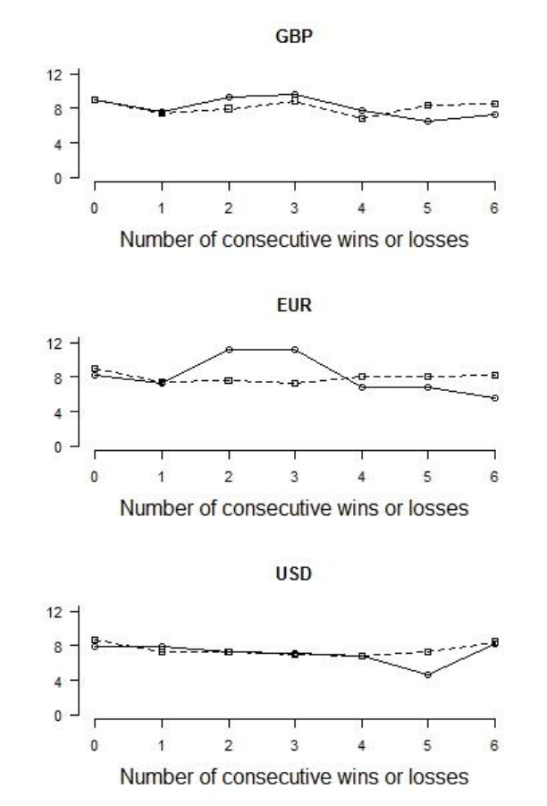
57
Figure 5. Mean odds plotted against streak length. The continuous line with the “o”
symbol shows data for consecutive wins and the dotted line with the “▢” symbol
shows data for consecutive losses.
One-way between-groups analyses of variance were carried out to determine
whether the odds that gamblers selected depended on the longest winning or losing
streak that they had experienced. Separate analyses were performed for winning and
losing streaks in EUR and USD (Figure 5). None of these six analyses showed a
significant effect of maximum streak length.
Odds
Odds
Odds
Odds
Odds
Odds
58
Replication of the original effect within each gambler
We then performed analyses to replicate the original effect within each
gambler. Thus, our question was whether individual gamblers tend to select safer
odds after experiencing longer winning streaks and riskier odds after experiencing
longer losing streaks. We used repeated measures analyses of variance to examine
the effect of the length of the winning streak experienced by a gambler on the odds
selected by that gambler. These showed the expected effects for GBP (F (1, 396,845)
= 4.73; p = 0.03), EUR (F (1, 161,791) = 17.21; p < 0 .001), and USD (F (1, 32,483)
= 4.48; p = 0.04). A similar repeated measures analysis for losing streaks showed the
expected effects for GBP (F (1, 365,226) = 21.65; p < 0.001) and EUR (F (1,
161,788) = 9.17; p = 0.003) but not for USD (F (1, 32,480) = 0.45; p=0.50 NS). As
in my original analysis, I attribute the failure to obtain a significant losing streak
effect for USD to the relatively small sample size.
Conclusions
There was no sign that gamblers who experienced longer winning streaks
generally placed safer bets or that gamblers who suffered longer losing streaks
generally placed riskier bets. In other words, there was no evidence of a selection
effect. Furthermore, we have shown that, within individual gamblers, increasingly
safe odds are chosen as winning streaks increase in length and increasingly risky
odds are chosen as losing streaks increase in length. This reinforces my original
conclusion and is not consistent with a selection effect. In summary, gamblers
became safer only after they had experienced winning streaks and became riskier
after they had experienced losing streaks. People who won were more likely to win
again because they chose safer odds than before and those who lost were more likely
to lose again because they chose riskier odds than before. However, selection of
59
safer odds after winning and riskier ones after losing indicates that online sports
gamblers expected their luck to reverse: they suffered from the gamblers’ fallacy. By
following in the gamblers’ fallacy, they created their own hot hands.
60
Chapter 5. A roulette experiment
In the chapter 4, sports gamblers showed a tendency of choosing lower odds
after longer winning streaks and higher odds after longer losing streaks. They
appeared to believe in gamblers' fallacy. By choosing lower odds, the winners won
more often and created a hot-hand effect. By choosing riskier odds after losing, the
losers lost more often. They created their own luck. If this self-fulfilling prophecy is
disrupted, what will happen? If choosing a safe bet no longer brings a safe result,
will people continue betting in a safe way? If a risky bet does not bring punishment,
what will happen? In this chapter, I will use a roulette experiment to answer these
questions.
Roulette requires no skill. It is a game of pure chance. The odds are
completely clear and transparent. The expected return of one unit of stake is -1/37
for European roulette and -2/38 for American roulette. Because of the
straightforward format of the gambling, roulette is a good game for discussion of the
hot hand and the gamblers' fallacies. In this roulette experiment, I aim to test whether
people’s gambling becomes more or less risky after winning or losing streaks.
Unknown to the gamblers, they experienced good or bad pre-determined ‘luck’.
They were chosen by the programme either to a long streak of winning or doomed to
lose for many times in a row.
5.1 Methodology
Participants
Participants were recruited online from Amazon Mechanical Turk. They
followed a link to a webpage with a roulette wheel. In total, 4712 people took part in
61
the experiment. Among them, 838 people used British pounds, 50 used Euros and
3824 used US dollars.
Design
The participants were randomly assigned to one of two groups: a ‘good luck’
group and a ‘bad luck’ group. They did not know there were such groups and they
did not know which group they were in.
Stimulus materials
Depending on the currency they chose, participants were presented with an
American or a European roulette wheel. Gamblers who used British pounds or Euros
were presented with European roulette and US dollar users were presented with an
American wheel. The American roulette wheel had 38 slots and the European one
had 37 slots. British, European and American participants were offered a notional
sum of £1000, €1000, or $1000, respectively, to gamble with.
Procedure
The first four rounds for each person were random. This gave them a chance
to become familiar with the roulette game and hopefully prevented them from being
suspicious of the predetermined rounds afterwards. From the fifth round to the 13
th
round, the gamblers in the ‘good luck’ group won nine times in a row no matter what
they bet on and those in the ‘bad luck’ group lost nine times in a row. Participants
were not made aware of the characteristics of the group to which they had been
assigned. They were told to try to make as much money as possible. The final reward
by lottery was positively related to how well they performed in the roulette game:
There was one winner chosen by a random lottery among all participants. The lottery
reward for the winner was £100*(percentile +1%). If the person who won the lottery
62
achieved a performance in the game that was better than 99% of the all the
participants, they received the full £100. If a person who won the lottery achieved a
performance in the game that was better than 50% of all the participants, they
received £51. Even if the participant did not win the lottery, they did not suffer real
losses. They only lost the fictional money which they were given at the beginning of
the game.
5.2 Results
The results show that people chose high odds in the first couple of trials but
that, very quickly, their odds dropped and then remained stable for the period in
which they experienced either winning streaks or losing streaks (Figure 6). Whether
participants experienced winning streaks or losing streaks did not change the odds
they bet on (Table 4).

63
Figure 6. Median odds change in always win (o) and always lose (Δ) rounds
.

64
Table 4. Regression for length of streaks predicting the median odds.
B
SE
df
t
Sig.(p)
F
𝑅
2
USD
Always
win
-0.06
0.01
18
-4.83
0.001*
23.28
0.54
Always
lose
-0.06
0.01
18
-6.25
0.001*
39
0.67
GBP
Always
win
-0.00
0.02
18
-0.18
0.86
0.04
-0.05
Always
lose
-0.00
0.01
18
0.00
1
0.00
-0.05
EUR
Always
win
-0.06
0.02
18
--3.84
0.001*
14.75
0.42
Always
lose
-0.08
0.02
18
-3.78
0.001*
14.23
0.41
Note: Independent variable is the length of streaks.
However, when gamblers experienced winning streaks, they increased the
stake size and when they experienced losing streaks, they decreased stake size. This
effect could have been the result of an increase or a decrease in their wealth (Figure
7).

65
Figure 7. Median stake change in always win (o) and always lose (Δ) rounds.

66
For USD and GBP players, though the effect of winning and losing streaks
on stake was significant, the effect sizes (𝑅
2
) were small. For Euro players, it was
not significant. This may have been due to the relatively small number of the Euro
players. It is difficult to claim how much influence the winning and losing streaks
had on the stakes. Particularly on the losing side, it seems the stake dropped to a low
level quickly and stayed there. It is possible that the stake had dropped to the lowest
possible. So the stake could not drop further as long as the participants were playing.
Table 5. Regression for length of streaks predicting the stake.
β
SE
df
t
Sig.(p)
F
𝑅
2
USD
Always win
13.64
0.92
7202
14.85
<.0001***
220.6
0.03
Always lose
-8.07
0.56
6637
14.41
<.0001***
208
0.03
GBP
Always win
12.4
2.22
1148
5.59
<.0001***
31
0.03
Always lose
-3.76
1.21
1231
-3.11
0.002**
9.67
0.01
EUR
Always win
9.15
8.62
104
1.06
0.29
1.13
0.01
Always lose
-7.28
7.27
75
-1.08
0.29
1.16
0.02
Note: Independent variable is the length of streaks.
The gamblers did not seem to change the odds or the stakes they bet on after
losing or winning. However, they changed which numbers they bet on (Table 6).
Binary regression was used to test whether winning or losing made gamblers change
the slots they bet on. For USD and Euro players, winning increased the chance that
they would change the slot that they bet on in the next round. However, for GBP
players, this effect was reversed: they preferred to stay with the same choice if they
won.

67
Table 6. Binary regression of winning and losing amounts predicting change of
chosen slot.
β
SE
df
z
Sig.(p)
USD
0.18
0.01
48338
18.95
<0.0001***
GBP
-0.08
0.02
9101
-3.33
<0.0001***
EUR
0.25
0.10
446
2.64
0.008**
Note: Independent variable is the winning and losing amounts.
5.4 Discussion
In this experiment, the winning or losing streaks did not affect the odds; the
streaks had a small effect on the stake. Gamblers using USD and Euro tended to keep
betting on the same slot on the roulette while gamblers using GBP tend to change the
slot when they win. Thus, there is some ambiguity about how gamblers react to the
always win and always lose situation in this experiment. They seemed not react to
the winning or losing results much. One possible explanation is that when playing
roulette, gamblers tend not to change the odds or the stakes; they are rather reacting
to other environmental stimuli, e.g. music, lights, movements, etc (Dixon, Trigg and
Griffiths, 2007; Schüll, 2013). In roulette, like in other kinds of machine gambling,
the presence of ‘flow’ could be important. Flow is a series of small fast simple
actions which gets immediate feedback (Csikszentmihalyi, 1997). Mechanical
gambling like roulette is particularly prone to create a flow because of the simplicity
of wagering a bet. The gamblers in this experiment could have been playing the
roulette under such flow conditions rather than reacting to the winning or losing
results.
68
Another implication is that the discovery found in the Chapter 4 may not
apply to roulette or other forms of mechanical gambling, because the whole
mechanism of the game and the motivation for playing it are different.
The participants in this experiment may have behaved differently from real
gamblers because they did not gamble with real money. This could be one of the
reasons that they seemed not react to the winning or losing results.

69
Chapter 6. Real expertise in gambling
It is believed by a lot of people that there is something you can do to be a
winner in gambling. Some gambling games involve outcomes that are almost
certainly random, e.g. lottery games and roulette. However, this does not stop people
trying to strive for good luck. Superstition is a strategy for those who believe in it. In
other kinds of games like sports gambling, the extent to which outcomes are random
is less clear. There is strong tradition of believing in expertise in sports gambling.
Numerous books, columns and websites provide tips for horse racing, football, and
other sports. Betting companies also sell past records to people who want to carry
out analyses. I mentioned in the Chapter 2 that there is evidence of real expertise in
card games, such as blackjack (Mezrich, 2002; Javarone, 2015; DeDonno and
Detterman, 2008; Turner, 2008) and in Texas Hold'em (Hannum and Cabot, 2009;
Fiedler and Rock, 2009). In blackjack, gamblers can use the card counting technique
to increase their chances of a positive expected return, though their chances of losing
money are still high. In Texas Hold'em, professionals perform better than non-
professionals. It is assumed that they have real expertise. In this case, the nature of
that expertise is less straightforward than in blackjack.
Some researchers have not found much evidence of expertise in sports
betting so far (Ladouceur, Giroux and Jacques 1998; Cantinotti, Ladouceur and
Jacques, 2004). Some find moderate evidence of insider knowledge (Crafts, 1985).
Some researchers have found that sports gamblers preferred long odds, which made
the shorts odds somewhat profitable, or at least, less unprofitable (Golec and
Tamarkin, 1998).
70
In this chapter, I will investigate the existence of expertise with the online
football and horse racing data. I will present two analyses. The first one examines
whether some gamblers consistently have better returns than fellow gamblers. The
second is designed to discover how they achieve better returns.
6.1 Is there real expertise? Yes.
Data set
In this analysis, the same online gambling data were used as in Chapter 4. In
order to examine the expertise within games, only horse racing and football were
chosen for study because these two games had the highest number of bets and
highest number of participants. There are 303,499 horse racing bets by 483 gamblers
and 172,336 football bets by 735 gamblers from January to December 2010.
Methodology
First, in each game, the data were separated into the 12 calendar months of
2010. Second, within each month, gamblers’ monthly return rates on their stakes
were ranked from high to low. The ranking was used to compare the performance
across different gamblers across months. If some gamblers could consistently rank
higher than other gamblers, it indicates real expertise. Third, in every month, those
gamblers who made positive returns were selected and their monthly returns in rest
of the year were examined. This was to test whether gamblers who made a profit in
one month replicated their success in other months.
Results
For all the gamblers, their mean return rate or median return rate was almost
all negative over the year as a whole (Table 7). This is not surprising. After all, it is
well know that gambling is not a good way to make a living. The returns or profits

71
mentioned in this chapter are all expressed in terms of the return rate rather than the
actual amount received to allow comparisons to be made between individuals or
between different months.
Table 7. Monthly median and mean returns in horse racing and football.
Horse racing
Football
Median return
Mean return
Median return
Mean return
Jan
-0.074
-0.033
-0.007
0.050
Feb
-0.054
-0.095
-0.030
-0.121
Mar
-0.033
-0.036
-0.030
-0.135
Apr
-0.059
-0.104
-0.047
-0.102
May
-0.069
-0.170
-0.004
-0.007
Jun
-0.053
-0.183
-0.103
-0.223
Jul
-0.036
-0.004
-0.029
0.005
Aug
-0.065
-0.201
-0.074
-0.164
Sep
-0.032
-0.090
-0.041
-0.149
Oct
-0.055
-0.138
-0.038
-0.077
Nov
-0.115
-0.201
-0.064
-0.173
Dec
-0.060
-0.127
-0.051
-0.182
In most months, except April and August, gamblers’ monthly performance
ranking in each month was correlated with the ranking in other months (Table 8).

72
Table 8. The performance ranking in horse racing in each month was correlated with
the rankings in the other months.
Result of the Reduction in Dispersion Test
Sig.(p)
𝑅
2
Jan
2.43
0.015*
0.33
Feb
3.29
0.001**
0.41
Mar
3.76
< .001***
0.44
Apr
1.23
0.29
0.20
May
4.17
< .001***
0.46
Jun
3.52
0.001**
0.42
Jul
2.82
< .001***
0.37
Aug
1.49
0.16
0.24
Sep
2.70
< .001***
0.36
Oct
4.40
< .001***
0.48
Nov
3.81
< .001***
0.44
Dec
2.77
< .001***
0.37
Note: Each row is a nonparametric rank regression. In each row, that month was the
dependent variable and the other months were the independent variables.
Ranking provides a better measurement of performance than the return on
stake itself because it relates the performance of each individual to that of other
fellow gamblers. The reduction in dispersion test is a nonparametric test can be used
with rankings (Kloke and McKean, 2014). It provides a measure of fit for the whole
nonparametric regression. The calculation was performed using R software using the
Rfit function. When the ranking for January was the dependent variable, all other
73
months together explained 0.33 of the variance in ranking order of that month. If the
performance ranking in February had been singled out to predict the January
ranking, it may not have been significant and similarly for the rankings for March, or
April and so on. However, all the performance ranking lists from February to
December together predicted 0.33 of the ranking in January. In Table 8, each row is
the performance ranking of that month correlated with performance rankings of all
the remaining eleven months. The ranking of each month takes turns as the
dependent variable and as an independent variable. The results show that, apart from
April and August, performance rankings of all other months are significantly
correlated with those of the remaining months.
Table 8 shows that gamblers' performance levels in each month were
correlated. However, if they were just losing money stably every month, this could
hardly be called expertise. They may appear to perform better than peers, but one
simple strategy can beat them - not gambling at all. It is indeed better to lose less
than to lose more. But it is even better not to lose at all.
The next question is: For gamblers who made positive returns in a particular
month, how did they perform in other months? I analysed only the gamblers who
made a profit in at least one month during the year. Because most of the gamblers
did not make profit in any month, regressions would not be useful when most
months’ profits were zero. As a result, greater insight into the issue of whether there
is real expertise in gambling can be obtained by examining only the gamblers who
made profit rather than all the gamblers. (Examining the gamblers who mostly lost
would not offer new information – it would reveal only that people lose money when
gambling, which would not be a new discovery.) In the analysis that I report here,
74
when a gambler made profit in one month, their returns in all other months, no
matter whether they were profit or loss, were included in the analysis. Table 9 shows
that, for eight months in 2010, among gamblers who made profit for at least one
month, returns in horse racing in those months were correlated with returns in all
other eleven months.

75
Table 9. Positive returns in horse racing in one month were correlated with positive
or negative returns in other months.
Residual
standard
error
Residual degrees of
freedom
F
Sig.(p)
Adjusted 𝑅
2
Jan
0.10
10
2.61
0.071
0.46
Feb
0.62
11
6.66
0.002**
0.74
Mar
0.07
11
7.29
0.001**
0.76
Apr
0.08
10
7.00
0.002**
0.76
May
0.05
10
62.99
<.0001***
0.97
Jun
0.16
18
8.39
<.0001***
0.74
Jul
0.11
21
1.82
0.11
0.22
Aug
0.22
16
5.63
0.001**
0.65
Sep
0.24
15
0.63
0.77
-0.18
Oct
0.13
9
5.09
0.011*
0.69
Nov
0.03
7
91.04
<.0001***
0.98
Dec
0.54
15
1.60
0.20
0.20
Note: Each row is a linear regression of the monthly returns. In each row, that month
was the dependent variable and the other months were the independent variables.
Residual degrees of freedom refers to the number of values that are free to vary to in
a calculation. A high number for degrees of freedom indicates a large sample size.
Gamblers who made a positive return in one month were also likely to make
a profit in other months, or make a smaller loss. The residual standard error
76
measures the fit of the linear regression as a whole. As with the ranking test, if the
performance ranking in January had been singled out to predict the February
ranking, it might not have been significant and neither might the performance
rankings of March, or April and so on. However, all the performance rankings from
January and from March to December together could predict 0.74 of the variance of
the ranking in February.
The analysis of the football data shows similar results. For each month, gamblers’
monthly return rates on their stakes were ranked from high to low. The ranking was
used to compare the performance of different gamblers across months. If some
gamblers consistently rank higher than other gamblers, the analysis indicates real
expertise. Again, each month's ranking could be predicted collectively by other
months (Table 10).

77
Table 10. Performance ranking in football in each month was correlated with the
rankings in the other months.
Result of the Reduction in Dispersion Test
Sig.(p)
𝑅
2
Jan
2.74
<.001***
0.31
Feb
1.90
0.05
0.24
Mar
3.69
<.001***
0.38
Apr
0.42
<.001***
0.41
May
3.82
<.001***
0.39
Jun
4.91
<.001***
0.47
Jul
2.84
<.001***
0.32
Aug
3.48
<.001***
0.36
Sep
3.18
0.002**
0.34
Oct
3.31
0.001**
0.35
Nov
0.68
0.75
0.10
Dec
2.01
0.04*
0.25
Note: Each row is a nonparametric ranking regression. In each row, that month was
the dependent variable and the other months were the independent variables.
Football gamblers who made a profit rather than loss in a given month could
also be predicted from the returns on their stakes in the other months. In Table 11,
instead of rankings, the return rates were entered into the regressions.

78
Table 11. Positive returns in football in one month was correlated with positive or
negative returns in other months.
Residual
standard
error
Residual degree of
freedom
F
Sig.(p)
Adjusted 𝑅
2
Jan
0.15
27
3.15
0.007**
0.38
Feb
0.13
28
3.96
0.002**
0.45
Mar
0.12
21
1.71
0.140
0.20
Apr
0.19
29
1.39
0.228
0.10
May
0.23
32
10.35
<.0001***
0.70
Jun
0.12
17
4.76
0.002**
0.60
Jul
0.29
23
3.39
0.007**
0.44
Aug
0.27
17
2.83
0.026*
0.42
Sep
0.20
12
1.24
0.360
0.10
Oct
0.11
22
12.26
<.0001***
0.79
Nov
0.21
24
3.06
0.011*
0.39
Dec
0.08
23
4.33
0.001**
0.52
Note: Each row is a linear regression of the monthly returns. In each row, that month
was the dependent variable and the other months were the independent variables.
6.2 What is real expertise? The ability to control loss.
This analysis focussed on the difference between gamblers who made a profit
and those who made a loss. It was done by investigating loss chasing patterns. Loss
chasing is a major characteristic of problem gambling according to Diagnostic and
Statistical Manual of Mental Disorders, 5th edition (DSM-5) (American Psychiatric
Association, 2014). Problem gamblers want to win back money after losing streaks
by betting again but this can lead to further loss.
79
Data set
Exactly same data set was used as in section 6.1.
Methodology
The gambling records of each gambler over the whole year were arranged in
time order. When a gambler kept playing, the records were included in a single
session; if they stopped gambling for more than 24 hours, the session was considered
to be terminated. When they started to play again after a break, a new session was
considered to have started. Within each session, losing streaks were counted. For
example, if a string of gambling records was WIN WIN WIN LOSE LOSE LOSE
LOSE LOSE LOSE, and there was no gap longer than 24 hours between any single
game, the loss chasing values were 0, 0, 0, 1, 2, 3, 4, 5, 6. This gambler stopped
playing when the loss chasing value was 6. In other words, he stopped playing when
he had lost six times in a row . If a string of gambling records were WIN, WIN,
WIN, LOSE, LOSE, LOSE, LOSE, 25hr gap, LOSE, LOSE, the gambler played two
sessions. The loss chasing values in the first session were 0, 0, 0, 1, 2, 3, 4. He
stopped playing when he had lost four times in a row in the first session. The loss
chasing values of the second session were 1, 2. He stopped playing when he had lost
twice in a row in the second session. A gambler who stops playing at a loss chasing
value of 6 is considered to have a more serious loss chasing problem than a gambler
who stops at loss chasing value of 4 or 2. This analysis examines whether gamblers
who made profits from gambling were involved in less loss chasing than gamblers
who did not.
Results
Profitable gamblers were defined as those who made profit in one particular
month. In the previous analysis in section 6.1, they had shown that they were more
80
likely to win in other eleven months as well. They were indeed less likely to chase
losses (Table 12). Wilcoxon rank sum tests were used to compare the mean loss
chasing value between profitable and unprofitable gamblers because loss chasing
value is a ranked variable.

81
Table 12. Profitable gamblers were less likely to chase loss.
Profitable gamblers
Unprofitable gamblers
Mean loss
chasing
value at
end of a
session
Mean odds
at the
beginning
of a session
/Mean odds
at the end of
a session
Mean stake
at the
beginning
of a session
/Mean
stake at the
end of a
session
Mean loss
chasing
value at
end of a
session
Mean odds
at the
beginning
of a session
/Mean odds
at the end of
a session
Mean stake
at the
beginning
of a session
/Mean
stake at the
end of a
session
Jan
1.52
10.13/9.27
79/83
1.75
7.03/6.22
110/107
Feb
1.62
7.02/6.80
101/111
2.30
9.09/7.59
96/105
Mar
1.49
9.62/9.08
113/104
2.32
9.88/9.15
90/67
Apr
1.52
7.24/8.67
135/144
2.24
8.35/8.58
105/123
May
1.82
8.32/8.61
74/62
2.27
8.01/8.02
128/116
Jun
1.44
7.62/9.93
102/76
2.04
7.20/7.72
60/80
Jul
1.67
6.79/7.36
73/71
1.97
6.88/7.30
152/159
Aug
1.57
8.01/6.79
162/172
1.85
6.93/9.40
181/202
Sep
1.59
9.15/7.95
66/57
1.76
7.014/7.51
177/171
Oct
1.43
5.20/5.34
69/71
2.21
8.19/8.25
89/92
Nov
1.63
9.07/10.50
82/124
1.76
6.945/6.42
102/101
Dec
0.99
5.72/5.15
148/156
1.96
8.07/8.91
97/69
Whole
year
1.57
8.40/8.10
105/93
2.01
7.68/7.81
114/116
t = 0.54,
df = 22,
p = 0.59
NS
t = -0.17,
df = 21,
p = 0.87
NS
t = 0.15,
df = 22,
p = 0.88
NS
t = -0.04,
df = 22,
p = 0.97
NS
Wilcoxon rank sum test of loss chasing value at end of a session for profitable and
unprofitable gamblers: W = 3, p < .0001***
Independent t-test of mean odds at the beginning of a session for profitable and
unprofitable gamblers: t = 0.05, df = 19, p-value = 0.96
Independent t-test of mean odds at the end of a session for profitable and
unprofitable gamblers:
t = -0.49, df = 17, p-value = 0.63
Independent t-test of mean stake at the beginning of a session for profitable and
unprofitable gamblers: t = -1.07, df = 22, p-value = 0.30
Independent t-test of mean stake at the end of a session for profitable and
unprofitable gamblers:
t = -0.81, df = 22, p-value = 0.43
82
Table 12 shows that unprofitable gamblers had a higher loss chasing value
(W = 3, p < .0001***). This indicates that unprofitable gamblers quit gambling when
they were deep into loss chasing while profitable gamblers quit when they had not
successively lost so many times. An independent t-test showed that there was no
significant difference between mean odds at the beginning of a session between
profitable gamblers or unprofitable gamblers. There was also no significant
difference between mean odds at the end of a session between profitable gamblers or
unprofitable gamblers. In addition, there was no significant difference in mean stake
at the beginning of a session between these two types of gamblers. Neither was there
a significant difference between their stakes at the end of a session. Furthermore,
compared across profitable gamblers and unprofitable gamblers, the mean odds and
mean stake were not significantly different. (Because the comparisons were made
between profitable and unprofitable gamblers, rather than the same group of people
under different conditions, independent t-tests were used.)
Conclusion
The two analyses in this chapter show that some gamblers do have real
expertise. Their performance was stable compared to other fellow gamblers and they
made profits consistently across the whole year. In the second analysis, a potential
mechanism underlying this consistent profitability was identified. Gamblers who
made profits and gamblers who made losses were not different to start with. Their
odds and stakes were not different at the beginning or at the end of the sessions. The
main difference was that profitable gamblers did not chase losses as much as the
unprofitable ones. Loss control is the key to making consistent profits. Profitable

83
gamblers stopped earlier than unprofitable gamblers. They showed less loss chasing.
This is consistent with the stereotype of the loss chasing by problem gamblers.
Previous research has shown that gamblers who hold more accurate estimates
of the probability of winning are unlikely to chase loss (Svetieva and Walker, 2008;
Griffiths and Whitty, 2010); they also show lower levels of cognitive biases
(Gainsbury, Suhonen and Saastamoinen, 2014). Hence reduced levels of cognitive
biases, more accurate estimates of winning probabilities and less loss chasing are
correlated. A more rational person is likely to win more or lose less when gambling.
Real expertise derives from rational thought.
Obviously, limiting loss chasing do not guarantee winning. So why do some
gamblers actually make money rather than merely make a smaller loss than other
gamblers? The reason is unclear. It is possible that some gamblers have inside
information (Crafts, 1985). Unfortunately, from the data that we have, it is not
possible to differentiate between expertise and inside information.
All major gambling houses have used systems in which gamblers can set
limits on the own gambling behaviour. The findings outlined here could lead to other
strategies to prevent problem gambling. For example, detection of loss chasing could
enable the gambler or the gambling house to prevent it (Adami, Benini, Boschetti,
Canini, Maione and Temporin, 2013).
84
Chapter 7 Discussion and summary
Here I summarise the three main findings produced by the research reported
in this thesis.
7.1 Evidence for the hot hand but not for the gamblers’ fallacy.
In sports gambling, people were more likely to win after winning streaks and
more likely to lose after losing streaks. We found evidence for the hot hand.
However, gamblers appeared to believe in the gamblers' fallacy: After winning,
gamblers selected safer odds. After losing, they selected riskier odds. After winning
or losing, they expected the trend to reverse. By following the gamblers’ fallacy,
people created their own hot hand. This result is ironic: Winners were worried that
their good luck was not going to continue and so they selected safer odds. By doing
so, they became more likely to win. The losers expected their luck to turn and so
they took riskier odds. However, this made them even more likely to lose. The
gamblers’ fallacy created the hot hand.
Previous research have shown that people follow the gamblers' fallacy in
random events over which they have no control (Ayton and Fischer, 20014;
Oskarsson, Van Boven, McClelland and Hastie, 2009). Based on this research, the
present results imply that sports gamblers do not appear to believe that they have
control over the events they bet on. This is the opposite of the illusion of control. It
could be called the illusion of no control.
This discovery has implications for other domains, e.g., financial trading.
Traders reduce their preference for risk in the wake of chance success and thereby
give the impression of a hot hand. They may attribute their successes to skills rather
85
than chance and may not be aware of their change in risk preference. In such
circumstances, they may develop the illusion that they are becoming better at the
task and able to persuade others that this is so. In the financial domain, this would
have clear implications for people’s selection of investment strategies.
7.2 Gamblers behave differently in roulette and in sports gambling.
When playing roulette, there was little evidence that gamblers changed their
odds or their stake following winning or losing streaks. It was also unclear whether
they changed the nature of their bets. In other words, they did not appear to react
much to winning or losing. It is possible that roulette gamblers are enjoying things
other than the results of their gambling. This makes it difficult to compare sports
gambling and roulette gambling: these gamblers may be motivated by different
things. In sports gambling, every bet is unique: a new horse, a new game, a new bet.
The gambler always needs to make new choices. In contrast, this is not the case in
mechanical games like roulette. Other mechanical gambling games, such as playing
fruit machines, are likely to share more similarities with roulette than with sports
gambling.
7.3 There is real expertise in sports gambling: it is loss control.
Some gamblers consistently outperformed their peers. They also consistently
made higher profits or lower losses. This indicates either real expertise or use of
inside information. These profitable gamblers do not differ from unprofitable ones in
odds that they prefer or in the stakes that they place. The key difference is that the
profitable gamblers did not chase their losses. Combined with other research, this
finding allows us to say that people with lower levels of cognitive biases and more
86
accurate estimates of winning probabilities show less loss chasing. This can be taken
to imply that a more rational person is more likely to win more or to lose less when
gambling. Thus, it appears that real expertise in gambling derives from the degree of
rationality possessed by the gambler. A rational gambler is a gambler that accepts
and cuts losses.
This discovery implies that a tool to detect loss chasing could provide an
effective means to prevent problem gambling.
87
References
Adami, N., Benini, S., Boschetti, A., Canini, L., Maione, F., Temporin, M., 2013.
Markers of unsustainable gambling for early detection of at-risk online
gamblers. International Gambling Studies 13 (2), 188–204.
http://dx.doi.org/10.1080/14459795.2012.754919
American Psychiatric Association, (2014), Diagnostic and Statistical Manual of
Mental Disorders (DSM-5®),
http://www.psychiatry.org/psychiatrists/practice/dsm/dsm-5
Andersson, P., Memmert, D., & Popowicz, E. (2009). Forecasting outcomes of the
World Cup 2006 in football: Performance and confidence of bettors and
laypeople. Psychology of Sport and Exercise, 10(1), 116-123.
http://dx.doi.org/10.1016/j.psychsport.2008.07.008
Ariyabuddhiphongs, V., & Chanchalermporn, N. (2007). A test of social cognitive
theory. Reciprocal and sequential effects : Hope, superstitious belief and
environmental factors among lottery gamblers in Thailand, Journal of
Gambling Studies, 23: 201–214. http://doi.org/10.1007/s10899-006-9035-3
Arkes, J. (2010). Revisiting the Hot Hand Theory with Free Throw Data in a
Multivariate Framework. Journal of Quantitative Analysis in Sports, 6(1).
http://doi.org/10.2202/1559-0410.1198
88
Ayton, P., & Fischer, I. (2004). The hot hand fallacy and the gambler’s fallacy: two
faces of subjective randomness? Memory & Cognition, 32(8), 1369–78.
doi:10.3758/BF03206327
Beckert, J., & Lutter, M. (2013). Why the poor play the Lottery: Sociological
approaches to explaining class-based Lottery play. Sociology, 47(6), 1152–
1170. http://doi.org/10.1177/0038038512457854
Bernoulli, D. (1954). "Exposition of a new theory on the measurement of risk". (Ed.
& Trans.) Econometrica 22 (1): 23–36. doi:10.2307/1909829. (Original work
published 1738)
Binde, P. (2013). Why people gamble: a model with five motivational dimensions.
International Gambling Studies, 13(1), 81–97.
http://doi.org/10.1080/14459795.2012.712150
Binswanger, H. P. (1981). Attitudes towards risk: Theoretical implications of an
experiment in northern India. The Economic Journal, 91, 364.
Blaszczynski, A., & Nower, L. (2002). A pathways model of problem and
pathological gambling. Addiction, 97, 487-499. http://doi.org/10.1046/j.1360-
0443.2002.00015.x
Bordalo, P., Shleifer, A., & Gennaioli, N. (2010). Salience theory of choice under
risk. National Bureau of Economic Research.
http://doi.org/10.1093/qje/qjs018.
89
Brickman, P., Coates, D., & Janoff-Bulman, R. (1978). Lottery winners and accident
victims: is happiness relative? Journal of Personality and Social Psychology,
36(8), 917–927. http://doi.org/10.1037/0022-3514.36.8.917
Bullock, S., & Potenza, M. (2013). Update on the pharmacological treatment of
pathological gambling. Current Psychopharmacology, 2(3), 204-211
Camelot, (2015). Retrieved 31 Dec 2015, from https://www.national-
lottery.co.uk/results/lotto/draw-history
Camelot, (2016a). Lotto, PLAYERS' GUIDE. Retrieved 7 March 2016, from
https://www.national-lottery.co.uk/games/in-store/players-guide/lotto
Camelot, (2016b). £4 Million Blue Game Procedures. Retrieved 7 March 2016, from
https://www.national-lottery.co.uk/c/files/scratchcards/4millionblue.pdf~2
Cantinotti, M., Ladouceur, R., & Jacques, C. (2004). Sports Betting: Can Gamblers
Beat Randomness? Psychology of Addictive Behaviors, 18 (2), 143-147.
http://dx.doi.org/10.1037/0893-164X.18.2.143
Carlton, P. L., Manowitz, P., McBride, H., Nora, R., Swartzburg, M. & Goldstein, L.
(1987) Attention deficit disorder and pathological gambling. Journal of
Clinical Psychiatry, 48, 487–488.
Casanova, G. (2013). The Story of My Life, Oxford, UK: Benediction Classics.
(Original work published in 1822)
90
Clark, L., Lawrence, A. J., Ashley-Jones, F., & Gray, N. (2009). Gambling near-
misses enhance motivation to gamble and recruit win-related brain circuitry.
Neuron, 61(3), 481–90. http://doi.org/10.1016/j.neuron.2008.12.031
Clotfelter, C. T., & Cook, P. J. (1991). Lotteries in the real world. Journal of Risk
and Uncertainty, 4(3), 227–232. http://doi.org/10.1007/BF00114154
Cook, P. J., & Clotfelter, C. T. (1991). The peculiar scale economies of lotto (No.
w3766). National Bureau of Economic Research. doi: 10.3386/w3766
Crafts, N. F. (1985). Some evidence of insider knowledge in horse race betting in
Britain. Economica, 52(207), 295-304. doi:10.2307/2553853
Croson, R., & Sundali, J. (2005). The gambler’s fallacy and the Hot Hand: Empirical
data from casinos. Journal of Risk and Uncertainty, 30(3), 195-209.
http://dx.doi.org/10.1007/s11166-005-1153-2
Csikszentmihalyi, M. (1997). Finding flow: The psychology of engagement with
everyday life. Basic Books.
DeDonno, M. A., & Detterman, D. K. (2008). Poker Is a Skill. Gaming Law Review,
12(1), 31–36. http://doi.org/10.1089/glr.2008.12105
Demaree, H. A., Weaver, J. S., & Juergensen, J. (2014). A fallacious “Gambler’s
Fallacy”? Commentary on Xu and Harvey (2014). Cognition, 139, 168-170.
http://dx.doi.org/10.1016/j.cognition.2014.08.016
91
Dixon, L., Trigg, R., & Griffiths, M. (2007). An Empirical Investigation of Music
and Gambling Behaviour. International Gambling Studies, 7(3), 315–326.
http://doi.org/10.1080/14459790701601471
Eisenegger, C., & Naef, M. (2011). Combining behavioral endocrinology and
experimental economics: testosterone and social decision making. Journal of
Visualized Experiments, (49). http://doi.org/10.3791/2065
Fiedler, I. C., & Rock, J.-P. (2009). Quantifying skill in games—Theory and
empirical evidence for Poker. Gaming Law Review and Economics, 13(1),
50–57. http://doi.org/10.1089/glre.2008.13106
Fischer, I., & Savranevski, L. (2015). Extending the two faces of subjective
randomness: From the gambler’s and hot-hand fallacies toward a hierarchy of
binary sequence perception. Memory & Cognition, 43(7), 1056–1070.
http://doi.org/10.3758/s13421-015-0523-5
Flood, J. M. (2017). Chapter 1 ASC 105 Generally Accepted Accounting Principles
(pages 1–24). Wiley GAAP 2017: Interpretation and Application of
Generally Accepted Accounting Principles. Somerset, NJ: John Wiley &
Sons
Fong, L. H. N., Law, R., & Lam, D. (2013). An Examination of Factors Driving
Chinese Gamblers’ Fallacy Bias. Journal of Gambling Studies
,
http://doi.org/10.1007/s10899-013-9390-9
92
Forrest, D., Simmons, R., & Chesters, N. (2002). Buying a dream: Alternative
models of demand for Lotto. Economic Inquiry, 40(3), 485–496.
http://doi.org/10.1093/ei/40.3.485
Gainsbury, S. M., Russell, A., Hing, N., Wood, R., Lubman, D., & Blaszczynski, A.
(2015). How the Internet is changing gambling: findings from an Australian
Prevalence Survey. Journal of Gambling Studies, 31(1), 1–15.
http://doi.org/10.1007/s10899-013-9404-7
Gainsbury, S. M., Suhonen, N., & Saastamoinen, J. (2014). Chasing losses in online
poker and casino games: Characteristics and game play of Internet gamblers
at risk of disordered gambling. Psychiatry Research, 217(3), 220–225.
http://doi.org/10.1016/j.psychres.2014.03.033
Gambino, B., Fitzgerald, R., Shaffer, H., Renner, J., & Courtnage, P. (1993).
Perceived family history of problem gambling and scores on SOGS. Journal
of Gambling Studies, 9(2), 169-184. doi:10.1007/BF01014866
Gambling Commission, (2012) Machine standards category B3 & B4.
http://www.gamblingcommission.gov.uk/pdf/machine%20standards%20cate
gory%20b3%20and%20b4%20june%202012%20revision%202.pdf
Gardner, J., & Oswald, A. J. (2007). Money and mental wellbeing: A longitudinal
study of medium-sized lottery wins. Journal of Health Economics, 26(1), 49–
60. http://doi.org/10.1016/j.jhealeco.2006.08.004
Gilden, D. L., & Wilson, S. G. (1995). Streaks in skilled performance. Psychonomic
Bulletin & Review, 2(2), 260-265. http://doi.org/10.3758/bf03210967
93
Gilovich, T., Vallone, R., & Tversky, A. (1985). The hot hand in basketball: On the
misperception of random sequences. Cognitive Psychology, 17(3), 295–314.
http://doi.org/10.1016/0010-0285(85)90010-6
Goldstein, L., Manowitz, P., Nora, R., Swartzburg, M., & Carlton, P. L. (1985).
Differential EEG activation and pathological gambling. Biological
Psychiatry, 20(11), 1232-1234. http://dx.doi.org/10.1016/0006-
3223(85)90180-5
Golec, J., & Tamarkin, M. (1998). Bettors Love Skewness, Not Risk, at the Horse
Track. Journal of Political Economy, 106(1), 205-225. doi:10.1086/250007
Gooding, P., & Tarrier, N. (2009). A systematic review and meta-analysis of
cognitive-behavioural interventions to reduce problem gambling: Hedging
our bets? Behaviour Research and Therapy, 47(7), 592−607.
doi:10.1016/j.brat.2009.04.002.
Grant, J., Brewer, J., & Potenza, M. (2006). The neurobiology of substance and
behavioral addictions. CNS Spectrums, 11(12), 924-930.
http://dx.doi.org/10.1017/s109285290001511x
Griffiths, M. (1991). Psychobiology of the near-miss in fruit machine gambling. The
Journal of Psychology, 125(3), 347–57.
http://doi.org/10.1080/00223980.1991.10543298
Griffiths, M. (2000). Scratchcard gambling among adolescent males. Journal of
Gambling Studies, 16(1), 79–91. http://doi.org/10.1023/A:1009483401308
94
Griffiths, M. D., & Whitty, M. W. (2010). Online behavioural tracking in Internet
gambling research: Ethical and methodological issues. International Journal
of Internet Research Ethics, 3(12), 104-117.
Hannum, R. C., & Cabot, A. N. (2009). Toward legalization of poker: The skill vs.
chance debate. UNLV Gaming Research & Review Journal, 13(1), 1.
Hardoon, K. K., Baboushkin, H. R., Derevensky, J. L., & Gupta, R. (2001).
Underlying cognitions in the selection of lottery tickets. Journal of Clinical
Psychology, 57(6), 749–763. http://doi.org/10.1002/jclp.1047
Hodgins, D. C. (2005). Implications of a brief intervention trial for problem
gambling for future outcome research. Journal of Gambling Studies (Vol.
21, pp. 13–19). http://doi.org/10.1007/s10899-004-1917-7
Holtgraves, T., & Skeel, J. (1992). Cognitive biases in playing the Lottery :
Estimating the odds and choosing the numbers representativeness. Journal of
Applied Social Psychology, 22(12), 934–952. http://doi.org/10.1111/j.1559-
1816.1992.tb00935.x
Hurley, W. J., & Pavlov, A. (2011). There will be blood: On the risk-return
characteristics of a blackjack counting system. Chance, 24(2), 47–52.
http://doi.org/10.1007/s00144-011-0019-4
Jacobs, D. F. (1988). Evidence for a common dissociative-like reaction among
addicts. Journal of Gambling Behavior, 4(1), 27-37.
doi:10.1007/BF01043526
95
Javarone, M. A. (2015). Is poker a skill game? New insights from statistical physics.
Europhysics Letters, 110(5), 58003. doi: 10.1209/0295-5075/110/58003
Kahneman, D., & Tversky, A. (1979). Prospect Theory: An analysis of decision
under risk, Econometrica, 47(2), 263–292. http://doi.org/10.1111/j.1536-
7150.2011.00774.x
Kahneman, D., Knetsch, J., & Thaler, R. (1991). Anomalies: The Endowment Effect,
Loss Aversion, and Status Quo Bias. The Journal of Economic
Perspectives, 5(1), 193-206. doi: 10.1257/jep.5.1.193.
Kloke, J., & McKean, J. W. (2014). Nonparametric statistical methods using R.
CRC Press.
Koehler, J. J., & Conley, C. (2003). The'Hot Hand'Myth in Professional
Basketball. Journal of Sport & Exercise Psychology, 25, 253.
Konstantinou, E., Liagkou, V., Spirakis, P., Stamatiou, Y., & Yung, M. (2005).
“Trust Engineering:” From requirements to system design and maintenance –
A working National Lottery System Experience. Information Security, 44-58.
http://dx.doi.org/10.1007/11556992_4
Ladouceur, R., Giroux, I., & Jacques, C. (1998). Winning on the Horses: How Much
Strategy and Knowledge Are Needed? The Journal of Psychology, 132(2),
133–142. http://doi.org/10.1080/00223989809599154
Ladouceur, R., Paquet, C., & Dubé, D. (1996). Erroneous perceptions in generating
sequences of random events. Journal of Applied Social Psychology, 26(24),
2157–2166. d: 10.1111/j.1559-1816.1996.tb01793.x
96
Langer, E. (1975). The illusion of control. Journal of Personality and Social
Psychology, 32(2), 311–328. http://doi.org/10.1037/0022-3514.32.2.311
Larkey, P. D., Smith, R. A., & Kadane, J. B. (1989). It's okay to believe in the “hot
hand”. Chance, 2(4), 22-30.
http://dx.doi.org/10.1080/09332480.1989.10554950
Lesieur, H. R., & Blume, S. B. (1987). The South Oaks Gambling Screen (The
SOGS): A new instrument for the identification of pathological
gamblers. The American Journal of Psychiatry, 144, 1184–1188. doi:
10.1176/ajp.144.9.1184
Lesieur, H. R., & Rothschild, J. (1989). Children of gamblers anonymous
members. Journal of Gambling Behavior, 5(4), 269-281. doi:
10.1007/BF01672428
Leung, K. S., & Cottler, L. B. (2009). Treatment of pathological gambling. Current
Opinion in Psychiatry, 22(1), 69-74. doi: 10.1097/YCO.0b013e32831575d9
Levy, H. (1994). Absolute and relative risk aversion: An experimental study. Journal
of Risk and Uncertainty, 8(3), 289-307.
Lin, S. A., Lyons, M. J., Scherrer, J. F., Griffith, K., True, W. R., Goldberg, J., &
Tsuang, M. T. (1998). Familial influences on gambling behavior: an analysis
of 3359 twin pairs. Addiction, 93(9), 1375-1384. doi: 10.1046/j.1360-
0443.1998.93913758.x
Loewenstein, G. F., Weber, E. U., Hsee, C. K., & Welch, N. (2001). Risks as
Feelings. Psychological Bulletin. http://doi.org/10.1037/0033-2909.127.2.267
97
Markel, T., La Fleur, B., and La Fleur, B., (2015) La Fleur’s 2015 World Lottery
Almanac.
Markowitz, H. (1952). The Utility of Wealth. Journal of Political Economy, 60(2),
151-158.
Matheson, V. A., & Grote, K. R. (2004). Lotto fever: Do lottery players act
rationally around large jackpots? Economics Letters, 83(2), 233–237.
http://doi.org/10.1016/j.econlet.2003.11.010
McManus, S., Meltzer, H., Brugha, T. T., Bebbington, P. P., & Jenkins, R. (2009).
Adult psychiatric morbidity in England, 2007 Results of a household survey.
The Health and Social Care Information Centre, Social Care Statistics., 1–
274.
McMullan, J. L., & Miller, D. (2009). Wins, winning and winners: the commercial
advertising of lottery gambling. Journal of Gambling Studies, 25(3), 273–95.
http://doi.org/10.1007/s10899-009-9120-5
Meyer, G., von Meduna, M., Brosowski, T., & Hayer, T. (2013). Is poker a game of
skill or chance? A quasi-experimental study. Journal of Gambling Studies /
Co-Sponsored by the National Council on Problem Gambling and Institute
for the Study of Gambling and Commercial Gaming, 29(3), 535–50.
http://doi.org/10.1007/s10899-012-9327-8
Mezrich, B. (2002). Bringing down the house: The inside story of six MIT students
who took Vegas for millions. New York: Free Press.
98
Neave, N., Laing, S., Fink, B., & Manning, J. T. (2003). Second to fourth digit ratio,
testosterone and perceived male dominance. Proceedings. Biological
Sciences / The Royal Society, 270(1529), 2167–72.
http://doi.org/10.1098/rspb.2003.2502
Nicolai, G., & Hilderman, R. J. (2009). No-limit texas hold'em poker agents created
with evolutionary neural networks. In 2009 IEEE Symposium on
Computational Intelligence and Games (pp. 125-131). doi:
10.1109/CIG.2009.5286485
Op de Macks, Z. A., Gunther Moor, B., Overgaauw, S., Güroğlu, B., Dahl, R. E., &
Crone, E. A. (2011). Testosterone levels correspond with increased ventral
striatum activation in response to monetary rewards in adolescents.
Developmental Cognitive Neuroscience, 1(4), 506–16.
http://doi.org/10.1016/j.dcn.2011.06.003
Oskarsson, A. T., Van Boven, L., McClelland, G. H., & Hastie, R. (2009). What’s
next? Judging sequences of binary events. Psychological Bulletin, 135(2),
262–285. http://doi.org/10.1037/a0014821
Potenza, M. (2014). The neural bases of cognitive processes in gambling disorder.
Trends in Cognitive Sciences, 18(8), 429-438.
http://dx.doi.org/10.1016/j.tics.2014.03.007
Potenza, M.N., Steinberg, M.A., Skudlarski, P., Fulbright, R.K., Lacadie, C.M.,
Wilber, M.K., Rounsaville, B.J., Gore, J.C., & Wexler, B.E. (2003).
Gambling urges in pathological gambling: A functional magnetic resonance

99
imaging study. Archives of General Psychiatry, 60(8), 828-836.
doi:10.1001/archpsyc.60.8.828
Reid, R. L. (1986). The psychology of the near miss. Journal of Gambling Behavior,
2(1), 32–39. http://doi.org/10.1007/BF01019932
Rottenstreich, Y., & Hsee, C. (2001). Money, Kisses, and Electric Shocks: On the
Affective Psychology of Risk. Psychological Science, 12(3), 185-190. doi:
10.1111/1467-9280.00334
Rudski, J. (2004). The illusion of control, superstitious belief, and optimism. Current
Psychology, 22(4), 306-315. http://doi.org/10.1007/s12144-004-1036-8
Scarne, J., (1961). Scarne’s Complete Guide to Gambling. Simon and Schuster, New
York, NY.
Schüll, N. (2012), Addiction by Design: Machine Gambling in Las Vegas,
Princeton, NJ: Princeton University Press.
Schwartz, D. G. (2013). Roll the bones: The history of gambling, New York:
Gotham.
Shefrin, H., and Statman, M. (1985). The disposition to sell winners too early and
ride losers too long: Theory and evidence, Journal of Finance, 40, 777-790.
doi: 10.1111/j.1540-6261.1985.tb05002.x
Smith, A. (1776). An Inquiry Into the Nature and Causes of the Wealth of Nations,
London: Strahan and T. Cadell.
100
Snell, J. L. (1982). Gambling, probability and martingales. The Mathematical
Intelligencer, 4(3), 118–124. http://doi.org/10.1007/BF03024242
Stanton, S. J., Liening, S. H., & Schultheiss, O. C. (2011). Testosterone is positively
associated with risk taking in the Iowa Gambling Task. Hormones and
Behavior, 59(2), 252–6. http://doi.org/10.1016/j.yhbeh.2010.12.003
Steenbergh, T. A., Whelan, J. P Meyers, A. W., May, R. K., & Floyd, K.., (2004).
Impact of warning and brief intervention messages on knowledge of
gambling risk, irrational beliefs and behaviour. International Gambling
Studies, 4(1), 3–16. http://doi.org/10.1080/1445979042000224377
Stenstrom, E., Saad, G., Nepomuceno, M. V., & Mendenhall, Z. (2011).
Testosterone and domain-specific risk: Digit ratios (2D:4D and rel2) as
predictors of recreational, financial, and social risk-taking behaviors.
Personality and Individual Differences, 51(4), 412–416.
http://doi.org/10.1016/j.paid.2010.07.003
Stewart, N., Chater, N., & Brown, G. D. (2006). Decision by sampling. Cognitive
psychology, 53(1), 1-26. http://dx.doi.org/10.1016/j.cogpsych.2005.10.003
Stinchfield, R., Govoni, R., & Frisch, G. R. (2007). A review of screening and
assessment instruments for problem and pathological gambling. In G. Smith,
D. C. Hodgins, & R. J. Williams (Eds.), Research and measurement issues in
gambling studies (pp. 179–213). Burlington, MA: Academic Press.
101
Svetieva, E., & Walker, M. (2008). Inconsistency between concept and
measurement: the Canadian Problem Gambling Index (CPGI). Journal of
Gambling Issues, 157-173. doi: 10.4309/jgi.2008.22.2
Sylvain, C., Ladouceur, R., & Boisvert, J. (1997). Cognitive and behavioral
treatment of pathological gambling: A controlled study. Journal of
Consulting and Clinical Psychology, 65, (5), 727 - 732.
Terrell, D. (1994). A test of the gambler’s fallacy: Evidence from pari-mutuel games.
Journal of Risk and Uncertainty, 8(3), 309–317.
http://doi.org/10.1007/BF01064047
Thaler, R., and Johnson, E. J. (1990) Gambling with the House Money and Trying to
Break Even: The Effects of Prior Outcomes on Risky Choice. Management
Science. 36, 643-660.
Turner, N. E. (2008). Viewpoint: Poker Is an Acquired Skill. Gaming Law Review
and Economics, 12 (3), 229–230. http://doi.org/10.1089/glre.2008.12305
Turner, N., & Horbay, R. (2004). How do slot machines and other electronic
gambling machines actually work?. Journal of Gambling Issues.11.
Retrieved 1 Dec 2016 from
http://jgi.camh.net/doi/abs/10.4309/jgi.2004.11.21
Tversky, A. & Fox, C.R. (1995). Weighing risk and uncertainty. Psychological
Review, 102 (2), 269-283.
102
Tversky, A., & Kahneman, D. (1973). Availability: A heuristic for judging
frequency and probability. Cognitive Psychology, 5(2), 207–232.
http://doi.org/10.1016/0010-0285(73)90033-9
Tversky, A., & Kahneman, D. (1992). Advances in prospect theory: Cumulative
representation of uncertainty. Journal of Risk and Uncertainty, 5(4), 297-323.
doi:10.1007/BF00122574
Van Holst, R. J., Van Den Brink, W., Veltman, D. J., & Goudriaan, A. E. (2010).
Brain imaging studies in pathological gambling. Current Psychiatry Reports,
12(5), 418–425. http://doi.org/10.1007/s11920-010-0141-7
Van Honk, J., Schutter, D. J. L. G., Hermans, E. J., Putman, P., Tuiten, A., &
Koppeschaar, H. (2004). Testosterone shifts the balance between sensitivity
for punishment and reward in healthy young women.
Psychoneuroendocrinology, 29(7), 937–43.
http://doi.org/10.1016/j.psyneuen.2003.08.007
Wagenaar, W. A., 1988, Paradoxes of Gambling Behaviour. Hove and London, UK :
Lawrence Erlbaum Associates Ltd.
Wardle, H., Moody, A., Spence, S., Orford, J., Volberg, R., Jotangia, D., …. (2011).
British Gambling Prevalence Survey 2010.
Wardrop, R. L. (1999). Statistical tests for the hot-hand in basketball in a controlled
setting. American Statistician, 1, 1-20.
Windross, A., 2003. The luck of the draw: Superstition in gambling. Gambling
Research, 15(1): 63–77.
103
Wohl, M. J. a., & Enzle, M. E. (2002). The deployment of personal luck:
Sympathetic magic and illusory control in games of pure chance. Personality
and Social Psychology Bulletin, 28(10), 1388–1397.
http://doi.org/10.1177/014616702236870
Xu, J., & Harvey, N. (2014). Carry on winning: the gamblers’ fallacy creates hot
hand effects in online gambling. Cognition, 131(2), 173–80.
http://doi.org/10.1016/j.cognition.2014.01.002
Xu, J., & Harvey, N. (2015). Carry on winning: No selection effect. Cognition, 139,
171–173. http://doi.org/10.1016/j.cognition.2015.02.008
Yaari, G., & Eisenmann, S. (2011). The hot (invisible?) hand: Can time sequence
patterns of success/failure in sports be modeled as repeated random
independent trials?. PloS one, 6(10), e24532.
http://dx.doi.org/10.1371/journal.pone.0024532
