Career Women and the Durability of Marriage

∗

Andrew F. Newman

†

Claudia Olivetti

‡

October 2018

Abstract

We study the relationship between divorce rates and female labor force attachment

in the US. Recent cross-sectional evidence from US states displays a robust negative

correlation between divorce and the rate of married female labor force participation.

We suggest that this pattern can be explained by increased bargaining ﬂexibility within

two-earner as against one-earner households. Both members of two-earner marriages

can use cash rather than less eﬃcient in-kind or promised transfers to re-adjust intra-

household allocations when compensating for preference shocks or changes in outside

opportunities, rendering their marriages more durable. Using retrospective and longi-

tudinal data, we show that all else equal, there is a lower propensity to divorce among

families in which the wife is a “career woman,” i.e. has a higher labor force attachment,

though these families seem to display no lower incidence of marital diﬃculties.

Keywords: divorce, bargaining, nontransferable utility, marital instability, female labor

force participation

JEL codes: J12, D13, J21

1 Introduction

Many people believe that families with a working wife are more prone to divorce than those

with a stay-at-home wife. Indeed, as women streamed into the labor force during the 1960s

and 1970s, divorce rates increased signiﬁcantly, and helped to cement the notion that mar-

ital instability and dissolution are costs of a gender-balanced workforce.

A look at more

current evidence, however, suggests that this view needs to be reconsidered. For example,

∗

Thanks to Daron Acemoglu, Claudia Goldin, Georg Kirchsteiger, Chiara Margaria, Zvika Neeman,

Victor-Rios-Rull, Dana Rotz, Alessandra Voena, Randy Wright and audiences at the NBER Summer Insti-

tute, Boston University, ECARES, Southampton, and the Barcelona Summer Forum for useful discussion.

Deborah Goldschmidt Marco Ghiani provided outstanding research assistance. We are grateful to our spouses

for contributing to variation in the data.

†

Boston University and CEPR

‡

Boston College and NBER

An example in the popular press is Noer (2006). We discuss scholarship on the question below.

Correlation= -.524

2 3 4 5 6 7

Divorce Rate (per 1000 population)

0.60 0.65 0.70 0.75 0.80

LFP Married Women

LFP is from the American Community Survey 5-year sample- 2005-2009.

Divorce rate is from the U.S. National Center for Health Statistics- National Vital Statistics Reports. We use the average over 2005-2009.

Missing observations on divorce rate for CA, IN and LA. For GA, HI and MN, divorce rate used is from 2000.

LFP rates of married women and divorce rates by state - 2005-2009

Figure 1: Divorce and married women’s labor supply, ACS 2005-2009

as displayed in Figure 1, there is actually a negative relationship between the divorce rate

and the rate of married female labor force participation (MFLP) across U.S. states. This

pattern is opposite to what would be expected if working wives were contributing on net to

marital fragility. And, as shown in Table 1 and discussed in the Appendix, this negative

correlation remains strongly signiﬁcant even after controlling at the state level for demo-

graphic, economic, and institutional variables that been shown to bear on divorce; examples

include levels of female education, age at ﬁrst marriage, family size, income inequality, fe-

male participation in male-dominated occupations, or the presence of community property

laws. Could it be then that the conventional wisdom is missing something? Might working

women be good for marriage?

Economic theory provides a simple answer. It predicts that households with two per-

manent earners will behave diﬀerently from those with only one because of diﬀerences in

the degree of transferability among household members. If a problem arises that lowers her

partner’s satisfaction with the marriage, an earner can compensate with money, or what is

the same thing, a balanced basket of market-procured and household-produced goods, while

a non-earner must compensate only with household-produced goods. Thus, compared to

a one-earner household with the same income, a two-earner household will be better able

to make the frequent adjustments to consumption needed to keep both partners happy in

the face of preference changes, problems with house or kids, or new outside opportunities.

Under mild assumptions about the distribution of these “preference shocks,” the result is

a marriage for the two earner household that is less likely to dissolve; more generally, this

marital durability is increasing in the equality of the partners’ earnings.

In this paper, we illustrate the theoretical argument for this “transferability eﬀect” and

then provide evidence suggesting that it is operative in US households. We base our investi-

gation on the Marital Instability over the Life Course (MILC), a longitudinal data set that

follows a representative sample of married couples over a twenty-year span (from 1980 to

2000) and records information about labor force participation, earnings, and other economic

and demographic characteristics, as well as a rich set of indicators of marital happiness.

The data let us confront the chief challenges to empirical detection and identiﬁcation of

the transferability eﬀect. First, in some households, causality may be running from the state

of the marriage to the labor supply decision, rather than the other way around. In particular,

there may be households where the marriage is unstable, and the woman is therefore working

either as a precaution (divorce is expected and she is investing in human capital or labor

market contacts) or to compensate for losses in husband’s income.

Such “remedial earners”

would tend to generate a positive correlation between working and divorce, obscuring the

negative relation predicted by the transferability eﬀect. Indeed, in the conclusion we discuss

how the presence of remedial earners may confound interpretation of the cross-sectional

evidence on female labor force participation and divorce and the policy implications to be

drawn.

We address this problem in two ways. First, we focus on “career women,” measured

variously, but basically deﬁned as those who are in the labor force a substantial fraction of

the time both before and during marriage.

Compared to remedial earners, career earners

have lower costs of generating cash and current incomes that are more closely tied to their

permanent incomes, both of which are attributes that facilitate the operation of the trans-

ferability mechanism. Second, we use panel data, particularly the distribution of earnings

within households, to follow couples over time and help tease out the remedial from the

career earners.

The second diﬃculty comes from possible selection eﬀects – a woman’s propensity to have

a career may be correlated with other attributes that lead her to have a higher quality and

therefore more durable marriage. We have already mentioned age at marriage and education

as examples, but there could be unobserved ones as well, such as character traits or match

Much of the literature, especially outside economics, refers to marriages that are unmarked by strife,

conﬂict, appeal to outside counseling and other indicators of low marriage quality as being highly “stable”;

we shall follow suit and reserve the term “durable” for marriages that have a low probability of divorce.

This is close to the notion of career woman as one who works regardless of marital status (e.g. Goldin,

1995); in 2000, over 85% of single women 25 to 34 were working, while only 70% of married women were.

There is a crucial inference problem that arises in cross-section or short-panel data. In a cross-section

of women we might observe that working women are more likely to be divorced, but this could simply

reﬂect their need to make up for lost income from the break up. Similarly, in a short panel in which data

are collected at only two dates, women who happen to anticipate a divorce in the near future may be

(temporarily) working at the ﬁrst date and be divorced at the second date. This could make it appear as

though working women contribute to marital fragility when in fact it is just an instance of precautionary or

remedial working.

quality that are correlated with career orientation. We handle this concern by exploiting a

battery of quality-of-marriage questions in our data that allow us to assess whether career

women in fact select into better marriages.

We ﬁnd that all else equal, those couples in which the women are more attached to

the labor force are less likely to divorce. Moreover, female labor force attachment has the

strongest stabilizing eﬀect in couples in which the woman earns close to 50% of family income.

However, we do not ﬁnd that these families have lower rates of marital disagreement. Taken

together, our results suggest that it is the ﬂexibility to accommodate disagreement, rather

than a reduction in its incidence, that is keeping two-career marriages together.

Literature

Existing explanations connecting divorce and MFLP are varied, but all suggest that MFLP

and divorce rates should covary. Most ﬁnd causality running from MFLP to divorce rates:

career women are more independent and therefore more willing to divorce, (Nock, 2001);

the incomes of husbands and wives are substitutes, making marriage between equals less

valuable (Becker, Landes, and Micael, 1977); or there is increased marital conﬂict within

career couples (Mincer, 1985; Spitz and South, 1985).

Some authors have suggested that the two trends reﬂect a spurious correlation: improve-

ments in home production technology, which both lowers the opportunity cost of working

and reduces the value of a marriage, have contributed to increased MFLP and to increases in

divorce (Ogburn and Nimkoﬀ, 1955; Greenwood and Guner, 2004). In recent work, Steven-

son and Wolfers (2007) suggest that other technological factors, such as the contraceptive

pill, and changes in the wage structure, that have been found to be important determinant

for the increase in labor force participation of married women might also be responsible for

a concurrent increase in divorce rates.

Finally, as already mentioned in conjunction with remedial earners, there is a possibility

that causality runs the other way, and there is indeed a signiﬁcant set of papers that ex-

plore this possibility. The earliest papers in this vein pointed out that in the face of high

divorce rates, married women have increased incentives to invest in careers, as a kind of self

insurance (Greene and Quester, 1982; Johnson and Skinner, 1986; Johnson 1994). Married

women’s labor force participation might also increase as the result of conﬂicting spousal

preferences towards the adjustment of marital consumption in the face of increased divorce

risk (Fernandez and Wong, 2014). Relatedly, an increase in divorce risk (as proxied by

the shift from mutual consent to unilateral consent divorce) might reduce the returns from

marriage-speciﬁc investments and increase the incentives to invest in labor marketable skills

(Stevenson, 2007), or can results in limited commitment within marriage and in a realloca-

Rasul (2006) suggests that changes in divorce law would have led to temporary increases in divorce that

would then have fallen back to trend levels, which have in fact been falling over the past twenty years; see

also Wolfers (2006). It is not clear whether this “pipeline” eﬀect can account for the whole trend over forty

years, and in any case it makes no connection between divorce and MFLP.

tion of resources inside the household that impact married women’s labor supply decision

(Voena, 2015).

As we will discuss, there is evidence that this causal link is operative for a substantial

fraction of women, enough to confound inference on the eﬀects of female work on marriage

durability. In fact, though all the theoretical links we have mentioned seems intuitive and

plausible, on balance empirical ﬁndings have been inconclusive, with diﬀerent mechanisms

seemingly predominating across data sets or over time (Stevenson and Wolfers, 2007; Kille-

wald, 2016).

Bertrand et al. (2015) provide evidence that some women display labor supply behavior

that eﬀectively ensures their shares of household income remain below 50%. This is consistent

with our own data in which high attachment women typically earn around 30-40% of the

household income, and there are no cases in which the wife’s earning exceeds 50%. Moreover,

our theory also suggests that should such counterfactual couples exist, their divorce rates

would be somwehat higher than those in which the woman earns closer to 50%.

In addition to re-examining the relationship between divorce and MFLP, this paper con-

tributes to a literature that seeks to distinguish empirically the eﬀects of varying degrees

of transferability within households and other institutions. It has long been understood

theoretically that the non- or imperfectly-transferable-utility case diﬀers radically from the

transferable-utility one in terms of both predicted behavior (intra-household allocations,

choice of organizational design in ﬁrms, sorting patterns, or investment behavior) and wel-

fare (Becker, 1973; Legros-Newman 1996, 2007; Peters and Siow, 2002). There has been

rather less work that derives practically testable implications of these diﬀerences (e.g., Cher-

chye, deRock and Vermuelen, 2015) or that implements them empirically (Udry, 1996).

The rest of the paper proceeds as follows: in the next section we present a simple model of

the transferability eﬀect. The main empirical analysis based on longitudinal data is presented

in Section 3. Section 4 oﬀers concluding remarks, with some discussion of trends and policy

implications.

2 Conceptual Framework

The purpose of this section is to provide a simple reduced form model that isolates the

transferability eﬀect in order to show how it aﬀects marriage durability. In the empirical

section we will, of course, have to take account of other eﬀects (some of which we have

already mentioned) that may eﬀect durability but whose logic is already well established in

the literature.

We employ the standard household bargaining framework in which the two decision

makers derive utility from private goods and a local public good that is enjoyed if and only if

Voena (2015) argues that whether the increase in divorce risk increases or decreases the labor force

participation of married women depends on the property division laws. Equitable distribution and unilateral

divorce, by rewarding the spouse with the lower share of marital resources, might incentivized lower married

women’s labor force participation.

they remain together. Assume that preferences can be represented by an additively separable

utility of the form u

(c)+φ, where c is a vector of private good consumption and φ represents

the utility of “local public goods” (LPG) derived from the marriage (companionship, children,

possible scale economies in housing or other private goods), representing the net beneﬁt of

remaining married.

Assume that preferences are monotone and that the indirect utilities

corresponding to u

If the couple were to divorce, they would

each obtain an autarky payoﬀ represented by the indirect utilities (v, I − v), where v is the

monetary earnings of one partner, and I − v that of the other.

Money facilitates transferability. There are several possible reasons for this. One is

that money enables the purchases of balanced bundles of consumption goods that may

be transferred between partners. In-kind transfers are less eﬃcient means of transferring

utility. The second reason, inspired by contract theory, is that money can be transferred

now, whereas in-kind payments may have to be transferred in the future. The monetary

transfers are thus less subject to moral hazard and other commitment problems than are

other means of intrahousehold transfers. Third, money enables an aggrieved party to directly

purchase a suitable good that may compensate for a loss of LPG utility rather than engaging

in costly bargaining to get the partner to do so.

Thus, utility transfers can be made one-for-one transfers with money. Beyond the limit

of monetary means, utility transfers are accomplished less eﬃciently: along the frontier, the

utility given up by one partner exceeds that gained by the other. Thus when one partner’s

utility is less than φ, the slope of the frontier is less than 1 in magnitude, while above φ + I,

the slope exceeds one. We assume these non-monetary means of making utility transfers are

equally eﬀective on the margin, given their level, for each partner: the frontier is symmetric

about the 45

-line.

Figure 2 illustrates the basic logic. Two households, 1 and 2, with equal incomes I and

equal initial realizations φ of the payoﬀs from the LPG, share a utility possibility frontier

). There is perfect transferability achieved by sharing earned income (so that the indirect

utilities are given by (y

+ φ, y

+ φ), where y

is the income used by by partner i to purchase

private consumption. The frontier illustrates the extreme case of no transferability once

earned income I has been exhausted. The households diﬀer only in the way in which earned

income is initially distributed. Household 1 has one earner: this is reﬂected by the utility

distribution that would occur if the household were to divorce, which is represented by the

autarky point A

. Household 2 has two (equal) earners, with autarky payoﬀs represented

by A

. Suppose that the households have reached an equilibrium allocation of private goods

Though φ might depend on income in some of these interpretations, we suppress that dependence here,

as we control for household income in both the theoretical and empirical analyses.

There is a signiﬁcant literature (e.g. Bergstrom and Varian, 1985) that studies restrictions on preferences

lead to such utility functions and to transferable utility possibility frontiers assuming that there is frictionless

trade between the partners in all goods. It is worth emphasizing that we are not so much concerned with this

issue as with money’s role in diminishing frictions such as transaction costs or moral hazard that would turn

a linear frontier into a nonlinear one; our basic point would remain valid even if preferences did not satisfy

the Bergstrom-Varian restrictions, though the computations would naturally be rather more complex.

I+ϕ"

(a) Only Household 1 divorces

I+ϕ"

(b) Only Household 2 divorces

Figure 2: Bargaining sets before and after preference shocks.

— we make no particular assumptions about the bargaining protocol they use except that

it does lead them to some point on their (constrained) Pareto frontier.

Now let each partner experience a “shock” to the payoﬀ from the LPG, indicated by the

dashed arrow 1 in panel (a) of the diagram. This could represent such things as a change

in how they feel about each other, the unexpected pleasure (or stress) from an additional

child, or since the LPG simply represents the partners’ net beneﬁts of being married to

each other, a change in outside opportunities. Following the shocks, there is a new utility

possibility frontier W

. Shocks could be positive or negative; in this case W

reﬂects a mild

negative shock for partner 1 and a rather large one for partner 2. The partners may be

induced to renegotiate the allocation of private goods following the change in LPG. As long

as the autarky payoﬀ vector is Pareto dominated by some point on the frontier, the couple

will remain married and settle on a payoﬀ allocation on the new frontier. But should the

autarky payoﬀ now lie “outside” the frontier, there are now no realizable net gains from

trade, and the couple will divorce. In the ﬁgure, the one-earner household 1 divorces, but

following the same shock, the two-earner household 2 remains married.

There are of course shock realizations that could result in divorce for Household 2 but

not for Household 1 (shock 2 in panel (b)). But under mild restrictions on the distribution of

shock values (namely, that large ones are less probable than small ones), this is a less likely

outcome, and averaging over all possible shocks, the result is that the 2-earner household’s

marriage is more durable. Though our focus in the empirical analysis is on the diﬀerence

between egalitarian households like the two-earner Household 2, and rather less egalitarian

ones like Household 1, it turns out that these same properties of shock distributions imply

that the relationship between earnings equality and marriage durability is monotonically

increasing.

To be a bit more formal, represent the household utility possibility frontier by (x, W (x)),

where W (x) is a continuous, strictly decreasing (therefore a.e.-diﬀerentiable), self-inverse

function on R, with W (x) = I + 2φ − x for x ∈ [φ, φ + I]. Elsewhere,

0 ≥ W

(x) > −1 a.e. on (−∞, φ) and W

(x) < −1 a.e. on (I + φ, ∞).

The self-inverse property W(W(x)) ≡ x captures the symmetry of the partners in their

(ex-ante) tastes for the LPG and for their ability to make utility transfers beyond those

eﬀectuated with monetary earnings. One partner earns v, the other earns I − v, where

0 ≤ v ≤ I. Thus v = I/2 is the egalitarian two-earner household, and v = 0 (or v = I) is

the one-earner household.

The value of the local public good is subject to a shock for each partner, after which

they renegotiate the intra-household allocation. Shocks are drawn independently from the

same distribution F (·) with support (−∞, ∞) and density f(·). The density f is log concave,

which is a convenient way to formalize the idea that larger shocks are (weakly) less likely

than small ones.

If the household divorces, each member gets an autarky payoﬀ equal to the indirect utility

of earnings, i.e., the autarky payoﬀ is (v, I − v). It is convenient to think of the shocks as

being added to the autarky payoﬀs rather than subtracted to the value of the public good.

As long as the shocks (, η) added to the autarky payoﬀs remain inside the frontier, that

is, I − v + η ≤ W(v + ), the marriage continues. Given , this happens with probability

F (W (v + ) − (I − v)), and the marriage’s durability – the probability that it stays together

– is then

D(v) =

∞

−∞

f()F (W ( + v) − I + v)d

One special case is worth noting. When W (x) = I + 2φ − x everywhere (full transfer-

ability), then the argument of F (·) is just 2φ − , i.e. the distribution of earnings within the

household, as well as their aggregate level, are irrelevant.

We now state and prove the main theoretical result.

Proposition 1 Suppose the household has income I and the value of local public good is φ

for each partner. Assume

(1) The household utility possibility frontier is symmetric, transferable on [I, I + φ] and

imperfectly transferable outside of [I, I + φ];

(2) Preference shocks are i.i.d. with log-concave density.

Then the durability of marriage is increasing in the equality of household earnings.

The density f is log-concave if log f is concave; this implies f (x)f (y) − f(x − δ)f(y + δ) ≥ 0 for x < y

and δ > 0, among other things; many commonly used distributions (including the uniform, normal, logistic,

and Laplace) have log-concave densities. See e.g., Bagnoli and Bergstrom (2005).

Proof We show that D(·) is increasing below I/2 and decreasing above I/2. Now,

(v) =

∞

−∞

f()f(W( + v) − I + v)(W

( + v) + 1)d.

Make the change of variable x ≡  + v; then

(v) =

∞

−∞

f(x − v)f(W(x) − I + v)(W

(x) + 1)dx.

Since W

(x) + 1 = 0 for x ∈ (φ, φ + I),

(v) =

−∞

f(x − v)f(W (x) − I + v)(W

(x) + 1)dx

∞

φ+I

f(x − v)f(W (x) − I + v)(W

(x) + 1)dx.

Use the change of variable ˆx = W (x) in the second term, and note that W (ˆx) = x, x = φ + I

implies ˆx = φ, and x → ∞ implies ˆx → −∞, to rewrite this as

(v) =

−∞

[f(x − v)f(W (x) − I + v) − f(x − I + v)f(W (x) − v)](W

(x) + 1)dx. (1)

Since x < W (x) on (−∞, φ] log-concavity of f implies f(x − v)f(W (x) − I + v) − f(x −

I + v)f(W (x) − v) ≥ 0 iﬀ v ≤ I − v, with strict inequality on a non-null set. Moreover,

(x) + 1 > 0 a.e. on (−∞, φ]. Thus, D

> 0 when v < I − v and D

< 0 when v > I − v,

as claimed. 2

Remark 1. Symmetry is the natural benchmark. But in the asymmetric case in which

one partner values the marriage more than the other, durability will tend to be maximized

at a point where that partner has a higher monetary income. A leading example of such

preferences is when one partner dislikes being in the labor force relative to remaining in

the home. If marriage allows this partner to remain at home, the distribution of earnings

is opposite to what it needs to be to maximize durability, reinforcing our contention that

marriages in equitable two-career households are the most durable.

Remark 2. It is not necessary that autarky payoﬀs equal the (indirect utility of) within-

marriage earnings: what matters is that the autarky payoﬀs corresponding to equal earnings

are equal and that the diﬀerence in the autarky payoﬀs is monotonically increasing in the

earnings diﬀerence.

Remark 3. The result is not merely about the role of inequality; transferability is also

important. Consider the extreme case where utility is strictly non-transferable from the

autarky point (i.e., the partners cannot transfer any income to the other). The couple’s

Pareto frontier is then the autarky point translated by the initial value of the LPG. Thus

the distribution of (non-transferable) earnings has no impact on the likelihood of divorce:

shocks that drive the autarky point northwest, southeast or northeast of the frontier result

in divorce, and this is independent of where the autarky point may be initially (moving the

autarky point implies a parallel movement of the frontier). By contrast, as we have seen,

when income is transferable, moving the autraky point has no eﬀect on the position of the

frontier, and equality maximizes durability. In this sense transferability and equality are

complements.

3 Empirical Analysis

The starting point of the analysis is to construct marital and employment histories for a

cohort of married couples and study how, all else equal, wives’ employment status aﬀects

the stability of a couple’s marriage over time. This requires the use of a panel data set

where we can follow a couple over a suﬃciently long period of time to distinguish women

who are temporarily working from those who are permanently working (hence labor force

attachment), as well as observe whether the marriage ultimately ends in divorce.

3.1 Data

We draw on the MILC data set that follows married couples over a 20-year span.

This data

set is very useful for our purposes as it was designed in order to examine the causes of marital

instability of a group of married individuals.

It consists of a national probability sample

of 2,034 married men and women under 55 who were interviewed by telephone for the ﬁrst

time in the fall of 1980. They were re-interviewed ﬁve times, which generated a total of six

waves of data, collected in 1980, 1983, 1988, 1992-1994, 1997 and 2000. The characteristics

of the sample were compared with estimates made by the U.S. Census Bureau, and the 1980

sample was found to be nationally representative with respect to age, race, household size,

presence of children, region, and female participation to the labor market.

We select only couples who are in their ﬁrst marriages in 1980

and in which both spouses

are older than 18. We obtain a sample of 827 marriages of which 627 are still intact in year

2000, that is, 24% of the couples in our sample divorced by the end of the survey.

Our dependent variable is an indicator function equal to one if a couple is no longer

together by the end of the survey and zero otherwise. All the relevant time-varying variables

Booth, Johnson, Amato, and Rogers (2003), ICPSR Study No.: 3812: Marital Instability Over the Life

Course [United States]: A Six-Wave Panel Study, 1980, 1983, 1988, 1992-1994, 1997, 2000.

The paper most closely related to our study is Booth, Johnson, White and Edwards (1984). In this

paper the ﬁrst two waves of the survey are used to analyze the impact of wives’ employment on marital

instability (broadly deﬁned as the set of all divorce-related activities: from thinking about it to ﬁling for

separation/divorce). They ﬁnd a positive but small eﬀect of a wife’s hours of market work on marital

instability. But as suggested above, this is likely the result of the confounding eﬀects that a short panel

cannot distinguish.

Restricting the data analysis to ﬁrst marriages is a common assumption when studying marital outcomes.

See for example Isen and Stevenson (2010).

are updated to the last wave preceding divorce. For example, take a couple who divorced

between 1997 (wave V) and 2000 (wave VI). We record this couple as being divorced by the

end of the survey and record all the time-varying stock variables (e.g. marriage duration,

number of children, wife’s work experience) as of 1997. Averages and standard deviations of

the other relevant time varying variables (e.g. household earnings, earnings shares, qualita-

tive measures of the state of a marriage) for this couple are computed using information from

1980 (wave I) to 1997 (wave IV). Take instead a couple who divorced between 1992-94 (wave

IV) and 1997 (wave V), we record information for this couple as of wave IV and compute

averages over wave I to wave IV, and so forth. The reason for doing this is that, we we

do not know the relevant marriage-speciﬁc information at the time the marriage dissolved,

which for all couples in our sample occurs between surveys. For consistency, we use the same

rule, stopping in 1997, also for marriages still intact by year 2000.

Our baseline labor attachment construct (which we often will refer to as “High Attach-

ment”) is a dummy equal to 1 if a wife worked more than 75% of the marriage, and zero

otherwise. It is obtained by combining the information about whether the wife worked

post-marriage (as recorded in the 1980 survey), whether she has a job at the time of each

subsequent survey and whether she did any work in between each round of the survey. The

main construct excludes wife’s labor force participation before marriage, but we add this

information as a control in all the regressions. Approximately 68% of wives in our sample

are classiﬁed as having high labor force attachment according to this fairly loose measure of

the extensive margin of labor supply.

Nonetheless, our measure of High Attachment seems to capture essential features com-

monly associated with the notion of being a working or career woman. In Appendix Table

C2 (column 1 and 2) we show that High Attachment women are more likely to have attended

at least a few years of college. They earn more than Low Attachment women. However, as

shown in column 3 and 4 of Table C2, their husbands’ characteristics (education, earnings)

do not diﬀer systematically from those of men married to low attachment women. Moreover,

High Attachment women display a much lower volatility both in the earnings and earn-

ings share of household income (measured at the time of the survey) than Low Attachment

women.

We interpret this as capturing the fact that working women have current incomes

that are more closely tied to their permanent incomes, which is one interpretation of our

bargaining story.

As an alternative we also use a measure of attachment, which we call “Career,” based on

individual responses to a battery of qualitative questions. Speciﬁcally, we deﬁne Career = 1

if a respondent said that “pretty important” or “very important” reasons for wife working

were having a career, for a sense of accomplishment, for contact with other people and for

Our deﬁnition of attachment includes both part-time and full-time work. Unfortunately, we cannot

capture work intensity because information on work hours is available at the time of the survey but not for

all the years in between surveys.

The distributions are statistically diﬀerent from each other at the 1 percent signiﬁcance level based on

a Kolmogorov-Smirnoﬀ test.

ﬁnancial independence. According to this deﬁnition 64% of wives in our sample are career

women. Women who are classiﬁed as being career women according to this deﬁnition also

have, on average, higher wage characteristics than non-career women, but their husband

are not ‘better’ on any of the standard observable dimensions. Besides being higher on

average, their earnings and earnings share of household income exhibit a much lower volatility

than those of non-career women. The correlation between High Attachment and Career is

relatively high and statistically signiﬁcant (0.6, p-value=0.001). We interpret this as further

indication that our High Attachment measure captures essential features of being a career

woman.

Summary statistics for the sample are reported in appendix table C1. On average, wives

in our sample entered their ﬁrst marriage at age 20 and are 34 years old in the ﬁrst wave.

Husbands are on average two years older. Roughly 90% of the sample is white and 23% of

wives and 31% of husbands are college educated. Wives earn on average 22% of household

income. The wife is the respondent in 51% of the cases.

3.2 Results

The results using our benchmark measure of labor force attachment are reported in Table 1.

As previously discussed, the dependent variable is a dummy equal to one if the couple

divorced by the end of the survey and the main explanatory variable is an indicator function

equal to one if the wife was highly attached to the labor force during marriage.

Across all speciﬁcations (column 1 to 3), we ﬁnd that couples where the wife has a

stronger attachment to the labor market are signiﬁcantly less likely to divorce than couples

where the wife has a more intermittent participation to the labor force. Having a wife with

high labor force attachment decreases the probability that the marriage ends in a divorce

by 9 to 10 percentage points. Given that 24% of the couples in our sample are divorced by

year 2000, this is a sizable number. In column 4 to 6 we show that the results are robust to

dropping from the sample 76 marriages with missing information on the race of one or both

spouses.

We worry that a number of factors might be driving this correlation. For example,

more educated women are less likely to divorce than less educated women (Martin, 2005;

Isen and Stevenson, 2010), as well as more likely to work. Black women are more likely to

divorce than white women and tend to have slightly lower labor force participation (Isen

and Stevenson, 2010). In addition, Rotz (2013) shows that age at ﬁrst marriage has an

independent negative eﬀect on divorce. Thus in all speciﬁcations we add marriage duration

and age at ﬁrst marriage (of both spouses), and in Column 2,3, 5 and 6 we include an array

of control variables: husband’s and wife’s education (two dummies for having high school or

some college and being a college graduate), husband’s and wife’s race, number of children,

In our regressions, we set race equal to missing for these couples. Given the limited sample size we opted

for working with the largest possible number of observations. As shown in column 4 to 6 the results are very

similar whether we include these observations or not.

average family income and the average wife’s share of household income, both computed

over the length of marriage.

We ﬁnd that the coeﬃcient on our labor attachment variable does not change substan-

tially. The control variables that are statistically signiﬁcant have the expected sign. Divorce

is less likely the longer the marriage and if there are children in the household. Consistent

with Rotz (2013) we ﬁnd a negative correlation between the wife’s age at (ﬁrst) marriage

and divorce (though the estimate loose signiﬁcance once we add the richer set of controls).

Consistent with the results reported by Isen and Stevenson (2010), we ﬁnd that divorce rates

are lower for college-educated couples though the coeﬃcients are not statistically signiﬁcant.

We obtain similar results if instead of adding wife’s and husband’s education separately we

control for wife education and add indicators of husband’s educational attainment being

below or above that of his wife.

There are a number of additional concerns to be addressed. For example, our main

ﬁnding could be explained by diﬀerences in household wealth. Wealthier household have

more resources available for side payments. If households with a high attachment wife are

wealthier, this could be driving our result. In practice, most households in our sample have

very little wealth and, when they do, it is mostly in the form of illiquid assets (e.g. home

ownership). Another potential concern has to do with gender roles preferences. Fernandez et

al. (2004) argue that men whose mother worked are more likely to like and, therefore, marry

a working woman (relative to men who grew up with a stay at home mother). In addition,

they would be more likely to have socialized with women whose mother also worked. This

mechanism could potentially give rise to more stable marriages and explain our result. It

has also been suggested that lower occupational sex-segregation increases the meeting rate

with opposite sex co-workers, which could reduce marital durability (McKinnish, 2004). This

mechanism would work against our ﬁnding of higher marriage durability for working women.

In column 3 and 6 we show that including households assets, a measure of husband’s and

wife’s gender norm socialization (whether their mother worked full time during adolescence)

and a measures of the likelihood that the wife is in contact with male coworkers does not

change the point estimate.

In Table 1 we also ﬁnd that a higher wife’s share of family income is associated with

a higher probability of divorce. Since ‘High attachment’ women earn, on average, a larger

share of household income, 28% and 12%, respectively, this ﬁnding seems to be at odds with

our hypothesis. We argue that this is another instance of ‘precautionary working’. Low

attachment women whose marriage are in trouble are more likely to enter the labor market

and earn a higher share of household income right around the time of divorce. We will return

to this point in section 3.3.

We also performed a series of robustness checks of to assess the sensitivity of our results to

the way we deﬁne wife’s labor force attachment. In Table 2 we present the results obtained

using two alternative deﬁnitions of labor attachment. In column 1 and 2 we show that

including a woman’s pre-marital work experience in our calculation of labor force attachment,

if anything slightly increases the size of the main coeﬃcient. Having a high attachment wife

is associated with a 10 to 14 percentage points lower probability of divorce. This is about

two percentage points larger than the eﬀect estimated with our benchmark deﬁnition. In

column 3 to 6 we use our qualitative “career” variable as deﬁned above. Based on this

deﬁnition, a Career woman’s divorce probability is 4 to 7 percentage points lower than that

of a non-career woman. It is likely that, at least in part, this lower estimate is due to

the higher measurement error typically associated with qualitative indicators. In fact, the

estimate obtained for the sample where the wife responded to the career-related questions

are larger, though the diﬀerence between column 3-4 and 5-6 is not statistically signiﬁcant.

Since the MILC data set is small and relatively unexplored in economics we replicate our

analysis using data from the 2008 Survey of Income and Program Participation (SIPP) that

have been prominently used in this literature (e.g. Isen and Stevenson, 2010).

The results

of this analysis are discussed in Appendix B. The analysis conﬁrms our ﬁnding that, all else

equal, a woman with higher labor force attachment has a lower propensity to divorce.

The SIPP also allows us to explore whether our results can be explained by diﬀerences

across US states in divorce legislation. There is a large literature that studies the impact

of the changing divorce legislation on divorce rates and female outcomes (see Gray, 1998,

Stevenson, 2007, and Stevenson and Wolfers, 2007, for a survey). In recent work Voena

(2015) shows that women in unilateral divorce states with common property laws are less

likely to work and more likely to divorce. This could, in principle, explain our results.

We cannot use our MILC data for this robustness check because the information on state

of residence is only recorded in 1997 (the next to last wave), when almost all of the ever

divorced couples in our sample have already split. However, as shown in appendix Table B1

(column 5) our results using SIPP data are robust to the inclusion of state dummies for the

presence of community property and unilateral divorce.

3.3 Wife’s work, household inequality and divorce

In table 1 and 2 we ﬁnd that women who earn a larger share of income are signiﬁcantly

more likely to divorce. We argue that this ﬁnding is driven by the fact that we are mixing

two groups. On the one hand, career women work for the same reason that men work: to

provide for family, for ﬁnancial independence, or for personal satisfaction. On the other

hand, for women who are in the labor force “remedially,” the marriage is already rocky

(possibly because the husband loses his job or is disabled, but also for other reasons), and

the woman anticipates divorce. The wife works e to compensate for his lost earnings or to

prepare for working post-divorce. What these two very diﬀerent groups have in common is

We can construct a measure of a woman’s labor force attachment over the course of her marriage based

on retrospective information on both work history (from Topical Module 1) and marriage history (from

Topical Module 2).

The cross-state analysis if Table A1 also supports this conclusions.

0 .1 .2 .3 .4

Wife's contribution to family income

-4 -3 -2 -1

Waves before divorce

High attachment, divorced

Low attachment, divorced

High attachment, married

Low attachment, married

Figure 3: Share of household income by wife’s labor force attachment and marriage outcome

For divorced couples the x-axis measures waves preceding divorce. For married couple it indexes waves

preceding wave VI. So ”-4” is wave II, ”-3” wave III etc.

that the wife is working and likely earning a substantial share of the household income. But

they have very diﬀerent implications for the durability of marriage.

We start by showing in Figure 3 evidence suggesting that this distinction is operative

in the data. The ﬁgure plots wife’s earnings share by labor force attachment and marriage

outcomes (divorced, married). For couples who divorce, the last data point is the wife’s

earnings share in the wave preceding the marriage dissolution, the second to last is the wife’s

earnings share two waves before the separation, and so on up to fours waves before divorce

(this would be couples that divorced between 1992-94 and 1997). For couples who stay

together, the last point corresponds to 1997 and the ﬁrst to 1983.

As shown in the ﬁgure, the share of household income earned by High Attachment women

over the course of their marriage hovers around 30 percent and does not vary with the

marriage outcome (the blue lines do not diﬀer statistically). Low Attachment women (the

red lines) earn a much lower share of household income, around 10 percent. However, this

share increases to 30 percent about two waves before the marriage dissolves. This suggests

that Low Attachment women might be working remedially because their marriage is in

trouble and this remedial work also results in earning a higher income share.

Our model predicts that households that are more equal are more likely to stay together.

To get direct evidence for this prediction, in Table 3 we reports the results for a speciﬁcation

that includes a full interaction between High Attachment and a dummy variable that is equal

to one if the wife makes between 45 and 55 percent of household income (column 2 and 3). In

column 4 and 5 we run a similar speciﬁcation but deﬁne as being ’Equal Share’ households

There are only two couples who divorce between 1997 and 2000. So we drop the data point corresponding

to 5 waves before divorce and, for consistency, 1980 for never divorced couples.

where the wife makes 40 to 60 percent of household income. We ﬁnd that households in

which the wife is High Attachment have a 10 percentage point lower probability of breaking

up than a marriage to a Low Attachment woman. An equal share of family income further

reduces the likelihood of divorce of a High Attachment woman by 12 percentage points

(column 3) and the diﬀerence is statistically signiﬁcant. Consistent with the theory, this

eﬀect is smaller when we broaden the interval deﬁning an equal share household (column 5).

Summarizing the results from Table 1 to 3, we ﬁnd that high female labor force attach-

ment reduces the probability of divorce by about half, particularly when she earns close to

half of the total family income.

4 Do Career women have better marriages?

So far we have shown that career women’s marriages are more durable. There are a number of

alternative mechanisms that could be driving this results. For example, it could be the case

that career women diﬀer in some inherent characteristic from non-career women: maybe

they are generally more reliable, care more about children, or are intrinsically better at

compromising or negotiating, both in their jobs and in their marriages. Career women could

be choosier in their search for mates, taking longer to marry and consequently having higher

quality marriages. Dual-career marriages might face diﬀerent sources of stress from one-

career marriages, such as less time together in the household, or diﬀerential opportunities for

meeting new people (note these would have to result in less stress for dual-career households

to accord with our ﬁndings). Finally, the career women’s greater marriage durability could be

an artifact of sorting, whereby egalitarian households might somehow reﬂect better matching;

this would also account for why the equal earning households are the most durable. All

of these alternatives imply that we should observe evidence of higher marriage quality in

households where the wife is a career woman than in those in which she is not and that

quality should be increasing in equality of earnings. In order to tease out whether these

alternative mechanisms can explain our ﬁndings, we use MILC’s subjective indicators of

marital happiness/stability.

Table 4 reports the results obtained using the same speciﬁcation as in Table 1 and 2

but the dependent variable is now the average value (over the course of the marriage) of

diﬀerent indicators of marriage quality. Column 1 and 2 report results for the marital

instability index. This is a summary indicator of around forty items that measure thoughts

and behaviors tapping into some aspects of marriage instability. For example, whether the

respondent was thinking about divorce, if either spouse thought the marriage was in trouble,

whether either spouse had ever talked about marital problems with signiﬁcant others, friends,

clergy or counselors (see C for the full list). We ﬁnd that households where the wife has high

work attachment are not statistically diﬀerent from those where she is low attachment. The

same is true for marital happiness (column 3 and 4) and marital problems (column 5 and

6). Overall high-attachment marriages are as happy, or as unstable and problematic, as low

attachment ones.

The only control variable that is statistically signiﬁcant is whether the wife is the respon-

dent, which is signiﬁcantly associated with more stable (column 2) and happier (column 4)

marriages but more marital problem (column 6). This ﬁnding does not depend on the wife

being low-attachment (for example, it could be the case that low attachment women are

more likely to be at home). The correlation between high attachment and wife respondent

is positive but statistically insigniﬁcant (the correlation is 0.023 with p-value 0.51).

In Table 5 we examine three among the many sub-items used to compute the marital

instability summative score. We ﬁnd that high attachment marriages are signiﬁcantly more

likely to report either spouse having ever suggested a divorce or having talked to a friend,

clergy or counselor about marital problems, although the diﬀerence is not signiﬁcant once

we control for our baseline set of controls.

Female respondents are more likely to report

that they talked to someone about their marriage troubles (column 6, table 5).

Overall the evidence in table 4 and 5 suggests that high attachment marriages are not

better than low attachment marriages. If anything, they are more unstable.

Another way of looking at this is to show the evolution of the average quality of mar-

riages by wife’s attachment and marital outcome (Figure 4). The ﬁgure shows that, among

the divorced, the average quality of high and low attachment marriages does not diﬀer sig-

niﬁcantly during the years preceding a divorce (the red and blue solid lines). Marriages

that stay together are more stable, increasingly so over the course of the marriage (compare

the blue and red dashed lines). However, at any point over the life course high attachment

marriages are more stable on average than low attachment marriages. This goes counter to

selection stories implying higher quality marriages for high-attachment women. Comparing

Figure 4 to Figure 3 suggests that for low-attachment marriages ending in divorce marriage

instability leads the increase in wife’s income share. We interpret this as further evidence

that labor-force-unattached women might be likely to work because the marriage is in trouble

and not the other way around.

In Table 6 we study whether the average marital quality varies by attachment and intra-

household income equality. Panel A reports results for the three summary indicators dis-

cussed in Table 4, panel B for three marital instability sub-items in Table 5. We ﬁnd

that average marriage quality is lower in high-attachment unequal marriages than in low-

attachment marriages with similarly unequal income distribution (see column 1 and 3 in

Panel A, and column 2 and 3 in panel B). However, high attachment women in equal earn-

ings households are associated with lower instability or problems (and happier marriages).

The coeﬃcients are similar in magnitude to the direct eﬀect of high attachment but not

statistically signiﬁcant. It may not be very surprising that attached women who earn small

fractions of household income have somewhat less happy marriages (e.g., disappointment

relative to expectations particularly with respect to housework shares or career success),

It would be interesting to compare husband’s and wife’s responses but only the respondent is asked the

battery of qualitative questions. The respondent does not change across survey waves.

0 .2 .4 .6 .8

Index of Marital Instability

-4 -3 -2 -1

Waves before divorce

High attachment, divorced

Low attachment, divorced

High attachment, married

Low attachment, married

Figure 4: Marital instability by wife’s labor force attachment and marriage outcome

For divorced couples the x-axis measures waves preceding divorce. For married couple it indexes waves

preceding wave VI. So ”-4” is wave II, ”-3” wave III etc.

but the fact that the equal share attached women have somewhat better marriages should

dispel concerns that any aspects of the instability measures that are money-dependent (e.g

professional marriage counseling) are playing a signifcant role in our ﬁndings that attached

women have no more happy marriages than unattached ones.

Finally, in Table 7 we show that this indicators of marriage stability are indeed good

predictors of marital dissolution. The dependent variable is now the indicator function

for marriage ending in divorce (as in Table 1 to 3) and we control for marriage quality,

attachment and the interaction between the two. As expected, unstable marriages are more

likely to break up (column 1). However, consistent with previous ﬁndings, high attachment

wives are still signiﬁcantly more likely to stay married (column 2). The interaction term

between attachment and quality is of the right sign but not signiﬁcant.

We then use as the dependent variable the indicator measuring ”whether either spouse

thought the marriage was in trouble.” This is of easier interpretation relative to the index of

marital instability although it does not seem to be a good predictor of divorce for the average

couple in our sample either on its own (column 4) or having controlled for wife’s attachment

(column 5), which maintains its strong negative relationship to divorce. Column 6 reports

results for the speciﬁcation where we interact having thought the marriage was in trouble

and wife’s high attachment. The ﬁrst coeﬃcient in the column now measures the impact

that trouble has on the probability of divorce of low-attachment marriages. This eﬀect is

positive and signiﬁcant, implying a 13 percentage point higher probability of divorce relative

to low-attachment marriages that are not in trouble. On the other hand, high attachment

women whose marriage is in trouble are signiﬁcantly less likely to divorce.

One potential concern, as we have already suggested, is that the marital instability index

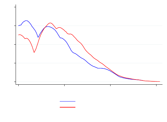
0 1 2 3 4

density

0 .2 .4 .6

Coefﬁcient of Mean Absolute Deviation

Low attachment

High attachment

Kolmogorov-Smirnov test: p-value=0.001

Figure 5: Distribution of within-marriage variability of Marital Instability Index by wife’s

labor force attachment

is endogenous (and that this explains why the marriage quality does not diﬀer by the wife’s

type): some parts of the instability measure (e.g. professional counseling) might be increased

by certain market purchases that only working women could access. We can address this

concern in another way: we repeat the analysis in Table 4-7 using the “initial” (i.e. as of

1980) battery of qualitative questions. The results are unchanged. Also, we note that the

indicator of marital problems is somewhat less ”endogenous” because it summarizes answers

to questions that don’t have a clear association with having money (for example, it captures

whether one or both spouses gets angry easily or gets easily hurt. See C for the full list of

sub-items.)

Finally, it could still be that high attachment marriages are ‘better’ than low attachment

marriages, even if they are on average the same or lower quality, because they are less

volatile. However, this does not seem to be the case in our data. As shown in Figure

5 high attachment marriages display a higher degree of variation in the index of marital

instability. The marital instability indicator includes items such as talking to a lawyer that

could be more easily purchased by high attachment wives. Thus in Figure 6 we show the

distribution of the coeﬃcient of variation (or absolute deviation) for the index of marital

problems, which, as we discussed above, can be thought of as being less aﬀected by having

money. In this case high and low attachment marriages exhibit the same degree of variation.

The two distribution are not statistically diﬀerent from each other.

Putting it all together: High attachment women do not seem to have intrinsically better

(higher quality and more stable) marriages. In fact, summary measure of marital instability

suggests that their marriages are more volatile.

0 .2 .4 .6 .8

density

0 1 2 3 4

Coefﬁcient of Mean Absolute Deviation

Low attachment

High attachment

Kolmogorov-Smirnov test: p-value=0.593

Figure 6: Distribution of within-marriage variability of Marital Problems Index by wife’s

labor force attachment

5 Conclusion

Economic theory predicts that two-earner households, particularly those with two career

workers with relatively equal incomes, ought to have the most durable marriages; we have

provided evidence that this prediction is borne out in practice. The basic mechanism is that

earners bring money – the most eﬃcient mode of utility transfer – into the household, which

maximizes the ﬂexibility to ﬁnd compensatory intra-household re-allocations in the face of

changes in preferences or outside opportunities.

We face two chief empirical challenges in trying to identify the transferability eﬀect

on divorce. One is to control for selection eﬀects, which we do with measures of number

of observable traits, as well as controls that measure marriage quality. The second is to

separate the eﬀect we are interested in, in which causality runs from female labor supply

to divorce, from the confounding eﬀect of divorce and marital instability on female labor

supply. This is accomplished by using a number of measures of female career attachment

that help distinguish wives who are permanent earners from those are remedial earners.

Once we do this we ﬁnd that all else equal, career women have 5-6 percent lower divorce

rate than non-career woman, that the eﬀect is strongest when women earn nearly the same

as their husbands, but that there is no evidence that career women select into higher quality

marriages.

The eﬀects of increased transferability, as well as the distinction between career and

remedial earning, has both positive and normative implications. On the positive side, it may

explain recent trends in divorce and MFLP. Since the mid 1980’s, U.S. divorce rates have

been declining. Meanwhile, MFLP has been increasing, leveling oﬀ with the 2008 ﬁnancial

crisis. This contrasts with the positive trend in both variables that lasted from the early

1960s to the mid 1980s and which no doubt helped spawn the large literature on female labor

and divorce. Could the transferability eﬀect account for the trend reversal? In principle it

might (see Neeman, Newman and Olivetti, 2007 for a theoretical attempt); moreover four

documented trends may have contributed to its increasing importance over time.

First, the gender wage gap has been closing, which corresponds to increased equality of

household earnings in our model. Second, the fraction of female workers who are career rather

than remedial earners has increased. As we have already pointed out, simply observing in

a cross section that a woman works could reﬂect remedial earning/marital instability rather

than career status: to the extent that the former is relatively less common now than in

the past, the rate of divorce should now be lower. Third, to the extent that the variety of

private goods enjoyed by household members can only be produced within the household

rather than purchased on the market, monetary earnings will be less eﬀective instruments of

utility transfer. It seems likely that over the period in question, there has been an increase in

the market availability of goods that are close substitutes for those produced in households

(for evidence on this “marketization” trend, see Freeman and Schettkat, 2005). Finally,

divorce laws, particularly those having to do with property division and alimony, evidently

aﬀect the post-divorce autarky payoﬀ, and therefore the durability of marriage. Greater

egalitarianism in these laws over the years may also have contributed to the trend reversal.

In short, for a variety of reasons, the transferability mechanism has likely strengthened over

the years, eventually overwhelming the countervailing eﬀects of MFLP on divorce that had

been the subject of other scholarship. Further research is needed to examine the extent to

which this conjecture is borne out quantitatively.

On the normative side, failing to control for the diﬀerence between career and remedial

earnings may confound inference about the eﬀects of female labor supply on divorce. Indeed,

the policy ramiﬁcations depend crucially on this distinction. For the woman who is contem-

plating joining the labor force after years of non-participation, the decision to enter is likely

a predictor of impending divorce. But for the young woman concerned about the impact of

working on her future family life, the best strategy for ensuring a durable marriage may be

to invest in a career.

Appendix 1. Decreasing shock densities

If the frontier W is concave, the conclusion of Proposition 1 can be established by substituting

log-concavity of f with the hypothesis that f is decreasing on [φ, ∞). To see this, observe

from (1) that D

(v) = 0 when v = I − v. Then the result follows if D

< 0 on [0, I].

Diﬀerentiate (1) to obtain

(v) =

−∞

[f(x − v)f

(W (x) − I + v) − f

(x − v)f(W (x) − I + v)](W

(x) + 1)dx

−∞

[f(x − I + v)f

(W (x) − v) − f

(x − I + v)f(W (x) − v)](W

(x) + 1)dx (2)

Use integration by parts to rewrite (2) as (perform the operation on the second terms in

each integral, using f(x − v) and f(W (x) − I + v)(W

(x) + 1) as the parts in the ﬁrst case

and f(x − I + v) and f(W (x) − v)(W

(x) + 1) in the second; then use lim

z→±∞

f(z) = 0 and

W (φ) = φ + I and regroup terms):

(v) = −f(φ − v)f(φ + v)(W

(φ) + 1) − f(φ − I + v)f(φ)(W

(φ) + 1)

−∞

f(x − v)f

(W (x) − I + v)(W

(x) + 1)

dx +

−∞

f(x − I + v)f

(W (x) − v)(W

(x) + 1)

−∞

f(x − v)f(W (x) − I + v)W

(x)dx +

−∞

f(x − I + v)f(W (x) − v)W

(x)dx

Since 1 + W

(φ) ≥ 0, the ﬁrst two terms are non-positive. Moreover, x < φ implies W (x) − v

and W (x) − I + v exceed φ, and since the density is decreasing on [φ, ∞), the second pair

of terms are negative. Finally, concavity of W (·) implies W

≤ 0 a.e., and we conclude

(v) < 0.

A Appendix: Evidence from the Census

We show that the negative relationship between the divorce and married women’s labor force

participation (MFLP) depicted in Figure 1 is robust to a number of state-level controls.

Table A1 presents the results, where we progressively add other factors.

Column 1 reports the regression coeﬃcient for the basic regression (this corresponds

to the correlation coeﬃcient reported in Figure 1). According to our estimate, which is

signiﬁcant at the 1% level, a state in which an additional 10% of the married women are in

the labor force than in another has 0.86 fewer divorces per 1000 people per year. Since the

average divorce rate is 3.6 per 1,000, this corresponds to a 24% reduction in the divorce rate.

Column 2 adds the marriage rate. The coeﬃcient is positive, reﬂecting the greater per capita

stock of marriages that can end in divorce. Nevertheless, the negative correlation between

divorce and labor force participation is unaﬀected, so it is not driven by hypothetically lower

In an earlier version of the paper we showed that the same negative correlation across US states is

observed based on Census 2000 data.

See below for a detailed discussion of data sources and variable deﬁnitions and Table A2 for summary

statistics. In all the regressions the state level variables are population-weighted.

marriage rates in states where more women work. MFLP, marriage rate, age at ﬁrst marriage

and education are all important: taken together they can explain 61 percent of the overall

cross-state variation in divorce rates.

The result is also robust to the inclusion of a number

of additional explanatory variables. For example, it has been suggested that higher male

income inequality increases the option value of a searching for a mate, which could result in

higher quality marriages (Loughran, 2002; Gould and Paserman, 2003). Moreover, there is

evidence that women in unilateral divorce states with common property laws are less likely to

work and more likely to divorce (Voena 2014). As shown in column 4 and 5, the correlation

between divorce and married woman LFP retains its sign and signiﬁcance even after having

controlled for all these factors.

Data sources.

Labor force participation, education, race, income, occupation, industry: 2005-2009 American

Community Survey (ACS). The sample is restricted to working-age population (16-64 years

old), not living in group quarters (GK=1). All state-levels averages and medians (for income)

are population-weighted. The “gender concentration” in industries/occupations is computed

as the percentage of working women in industries, occupations, and industry-occupation cells

where the state-level ratio of women to men is less than 50%. We use the 1950-adjusted

industry and occupation codes from the Census.

Marriage and divorce rates: U.S. National Center for Health Statistics, National Vital

Statistics Reports (NVSR), Births, Marriages, Divorces, and Deaths: Provisional Data for

2009, Vol. 58, No. 25, August 2010; and prior reports. Marriage and divorce rates used

for most states are for 2009 (the most recent). For states that didn’t report divorce rates

in 2009 we use the most recent available. That is, Georgia (2003); Hawaii (2002); Louisiana

(2003); Minnesota (2004). Since data for California are from 1990 and data from Indiana

are not available after 1980, we drop these two states from the main analysis. However, in

robustness checks we use the 1980s ﬁgure and we also use 2009 ACS data to estimate both

marriage and divorce rates.

Age at ﬁrst marriage: U.S. Census Bureau’s American Community Survey 2009, 1-year

estimates (from factﬁnder.census.gov).

Religion: 2007 ARDA (Association of Religion Data Archives) survey, www.thearda.com.

According to the site, “data [was] collected by representatives of the Association of Statis-

ticians of American Religious Bodies (ASARB).” Note that “While quite comprehensive,

this data excludes most of the historically African-American denominations and some other

major groups.” The ARDA survey reports missing values for Alaska, Hawaii and DC. For

these states, the information comes from Pew’s “U.S. Religious Landscape Survey” (2007’),

Column 5 omits Nevada, which leaves the results unchanged. We have experimented with alternative

measures of married women labor force participation, such as full- and part-time participation, labor force

participation of white women and labor force participation of 25-54 year old women. For all speciﬁcations

we obtain results similar to the ones reported here.

http://religions.pewforum.org/maps and http://religions.pewforum.org/reports.

Population density: Census 2010 -http://www.census.gov/geo/www/guidestloc/select data.html.

B Appendix: Evidence from the SIPP

Our measure of labor force attachment during marriage is obtained by matching information

on labor market interruptions (from the employment history module) with information on

marriage spells (from the marital history module). Unfortunately, the questionnaire does not

give any indication of when the time oﬀ was taken, making it diﬃcult to determine whether

a spell of non-employment occurred before, during, or after marriage, especially for women

whose ﬁrst marriage dissolved before the survey. In addition, it is not clear whether time

oﬀ is considered separately from time oﬀ spent caregiving, and one needs to avoid double-

counting any time oﬀ. Because of this limitation of the data, we exploit information on

start and end dates of employment and marriage to construct a binary indicator of whether

a woman worked at all during her ﬁrst marriage rather than more continuous estimates of

time spent working. This indicator takes a value of one if a woman started, but didn’t

stop, working before entering her ﬁrst marriage, or if she ﬁrst started working after her

ﬁrst marriage started but before it ended (if it ended). It takes a value of zero if she never

worked; if she worked, but stopped working before her ﬁrst marriage began; if she started

working only after her ﬁrst marriage ended; or if her time caregiving spanned her entire

marriage. While this indicator does not capture the intensity of labor force attachment

during marriage, it does not rely on ‘ad hoc’ assumptions and is relatively clean.

At the same time it seems to capture the essence of being a ‘career’ woman. As shown in

appendix Table B3, our measure of work during marriage is positively correlated with age

at ﬁrst marriage and at ﬁrst birth, conditional on having children during ﬁrst marriage, full-

time work and earnings (three alternative measures). ‘Career’ women are also more likely

to have a college or post-graduate degree, and to work in professional occupations.

We consider the sample of all women age 25-54, who are either in their ﬁrst or second

marriage, or separated/divorced by the time of the survey. We include in our sample only

marriages that occurred in the 1990s or later. This is to minimize the bias due to the

retrospective nature of our data and to make our sample as comparable as possible to that

used in our state cross section. Summary statistics for the sample are reported in appendix

table B2. Women in our sample are 37 years old, on average, 81% of then are white, 11%

are blacks and 6% asian, 57% of the women in our sample have at least a four-year college

degree. The entered their ﬁrst marriage when they were about 26 years old, on average, and

they have, on average, 1.94 children. Approximately thirty percent of all marriages in our

sample end in divorce; of these, the average marriage lasts ﬁve years, and 60% of divorces

occur by year 5.

The only errors in creating it came from observations for which the working end date comes before the

working start date. These observations have a missing value, but there are relatively few of them (41).

We report the regression results in Table B1. The dependent variable is the probability

that a marriage dissolves by year 5. Overall we ﬁnd that, all else equal, a marriage to a

career woman is about 6 percentage points less likely to end in divorce, which corresponds

to a 34% decline in the 5-year divorce probability.

The negative association between divorce and labor force attachment stands even after

having added controls for race, age at ﬁrst marriage, marriage duration, an indicator of

whether the couple had a child under the age of 6, an indicator of property division laws

in the current state of residence which is equal to one if the states has community property

(that is, is characterized by an equal distribution of property upon divorce independent on

title ownership) and a dummy equal to one if the state of residence has unilateral divorce

(as opposed to mutual consent).

Consistent with Isen and Stevenson (2010) we ﬁnd that

blacks are more likely to divorce. Finally, we ﬁnd that women who reside in states with

community property (who, except for Louisiana, also have unilateral divorce) are less likely

to divorce, while residing in a unilateral divorce state does not seem to aﬀect the probability

of divorce one way or another. This is consistent with ﬁndings by Wolfers (2006).

C Appendix: Marital Quality Measures in MILC data

In the analysis we use three main summary indicators of marital quality. We provide details

about their deﬁnitions and scale in this section.

Marital Instability

The Marital Instability index

is a summative score based on several items asked of married

people: feeling that marriage was in trouble; talking to others about marital problems; wish

of living apart from spouse; divorce thoughts; divorce suggestion from one of the spouses;

talking about consulting a divorce attorney; talking about property division; talking about

ﬁling; consulting an attorney; ﬁling a divorce or separation petition; occurrence of trial

separation; length of the last period of separation.

The index was logged and averaged over marriage years and it ranges between 0 and

1.31, with higher scores corresponding to greater marital instability and 50% of the couples

having an index below 0.24.

We also ran regressions looking at the probability of dissolution by year 7 and 10 as well as a Cox

proportional hazard model and found very similar results.

Obviously assigning divorce law by current state of residence rather than state of residence at time

marriage or divorce is not ideal. However, SIPP does not report this information so this is the most we can

do.

Booth, Alan, David Johnson, and John N. Edwards. 1983. ”Measuring Marital Instability.” Journal of

Marriage and the Family 45: 387-393.

Edwards, John N., David R. Johnson, and Alan Booth. ”Coming Apart: A Prognostic Instrument of

Marital Breakup.” Family Relations 36: 165-170.

Johnson, David R., Lynn K. White, John N. Edwards, and Alan Booth. ”Dimensions of Marital Quality:

Toward Methodological and Conceptual Reﬁnement.” Journal of Family Issues 7: 31-49.

In the analysis we also highlight three of the sub-items contributing to the marital insta-

bility summative score.

The variable Either Spouse Ever Suggested Divorce is a dummy equal to one if the re-

spondent answered ”yes” to the question: “Have you or your (husband/wife) ever seriously

suggested the idea of divorce?”

The variable Either Spouse Ever Talked About Marital Problems with Clergy, Counselor,

etc. is a dummy equal to one if the respondent answered ”yes” to any of the following

questions: “Have you ever talked with family members, friends, clergy, counselors, or social

workers about problems in your marriage? As far as you know has your (husband/wife)

talked with relatives, friends, or a counselor about problems either of you were having with

your marriage?”

The variable Either Spouse Thought Marriage was in Trouble is a dummy equal to one

if the respondent answered ”yes” to any of the following questions: “Even people who get

along quite well with their spouse sometimes wonder whether their marriage is working out.

Have you ever thought your marriage might be in trouble? As far as you know, has your

spouse ever thought your marriage was in trouble?”

Marital Happiness

The Marital Happiness index is a summative score based on several items capturing the

amount of happiness in the couple: extent of understanding received from spouse; amount

of love received; extent of agreement about things; sexual relationship; spouse as someone

who takes care of things around the house; spouse as someone to do things with; spouse’s

faithfulness; evaluation of marriage as very happy, pretty happy, or not too happy; compared

to other marriages, respondent’s is better, same, or not as good; comparing marriage to 3

years ago, it is getting better, staying the same, or getting worse; strength of feelings of love

respondent has for spouse.

The index was averaged over marriage years and it ranges between 13 and 33, with higher

scores indicating higher marital happiness and 50% of the couples having an index below

28.6.

Marital Problems

The Marital Problems index is a summative score based on several items capturing the

presence of marital problems because either or both spouses: gets angry easily; gets easily

hurt; is jealous; is domineering; is critical; is moody; won’t talk to the other; has sexual

relationship with others; has irritating habit; is not home enough; spends money foolishly;

drinks or uses drugs; has been in trouble with the law.

The index was averaged over marriage years and it ranges between 0 and 12, with higher

scores indicating greater marital problems and 50% of the couples having an index below

2.2.

References

[1] Bagnoli, Mark, and Ted Bergstrom (2005), “Log-concave probability and its applica-

tions,” Economic Theory 26:445-469.

[2] Becker, Gary S (1973), “A Theory of Marriage: Part I,” Journal of Political Economy

81: 813-846.

[3] Becker, Gary S., Elisabeth M. Landes, and Robert T. Michael (1977), “An Economic

Analysis of Marital Instability,” Journal of Political Economy, 85(6): 1141-1188.

[4] Bergstrom, Ted and Hal Varian (1985), ”When Do Market Games Have Transferable

Utility?” Journal of Economic Theory 35: 222-233.

[5] Bertrand, Marianne, Emir Kamenica and Jessica Pan (2015), “Gender Identity and

Relative Income within Households,” Quarterly Journal of Economics, 130(2): 571-

614.

[6] Bougheas, Spiros and Yannis Georgellis (1999), “The eﬀect of divorce costs on marriage

formation and dissolution,” Journal of Population Economics, 12(3): 489-498.

[7] Cherchye, Laurens, Thomas Demuynck, and Bram De Rock (2015), “Is utility transfer-

able? a revealed preference analysis”, Theoretical Economics, 10(1): 51-65.

[8] Freeman, Richard B. and Ronald Schettkat (2005), Marketization of Production and

the EU-US Gap in Work (Jobs and Home Work: Time Use Evidence),” Economic

Policy 20(41): 5-50.

[9] Goldin, Claudia (1995), “The U-Shaped Female Labor Force Function in Economic De-

velopment and Economic History,” in T. Paul Schultz, ed., Investment in Women’s

Human Capital and Economic Development. Chicago, IL: University of Chicago

Press, pp. 61-90.

[10] Gould, Eric D. and M. Daniele Paserman (2003), “Waiting for Mr. Right: rising inequal-

ity and declining marriage rates,” Journal of Urban Economics, 53(2): 257-281.

[11] Greene, William and Aline Quester (1982), “Divorce Risk and Wives’ Labor Supply

Behavior,” Social Science Quarterly 63(1): 16-27.

[12] Greenwood, Jeremy, and Nezih Guner (2004), “Marriage and Divorce Since World War

II: Analyzing the Role of Technological Progress on the Formation of Households,”

NBER Working Paper #10772.

[13] Gray, Jeﬀrey S. (1998), “Divorce-Law Changes, Household Bargaining, and Married

Women’s Labor Supply,” American Economic Review, 88 (3): 628-642

[14] Hakim, Danny (2006), “Panel Asks New York to Join the Era of No-fault Divorce,”

New York Times, Febraury 6.

[15] Isen, Adam and Betsey Stevenson (2010), “Women’s Education and Family Behavior:

Trends in Marriage, Divorce and Fertility,” http://www.nber.org/papers/w15725

Adam Isen, Betsey Stevenson

[16] Johnson, John H. (2004), “Do Long Work Hours Contribute To Divorce?,” John H.

Johnson, Topics in Economic Analysis and Policy.

[17] Johnson, William R., and Jonathan Skinner (1986), “Labor Supply and Marital Sepa-

ration,” American Economic Review 76: 455-469.

[18] Jovanovic, Boyan (1984), “Matching, Turnover, and Unemployment,” Journal of Polit-

ical Economy, 92(1): 108-22.

[19] Legros, Patrick, and Andrew F. Newman (2007), “Beauty is a Beast, Frog is a Prince:

Assortative Matching with Nontransferabilities,” Econometrica 75(4): 1073-1102.

[20] Lehrer, Evelyn (2008), “Age at Marriage and Marital Instability: The Becker-Landes-

Michael Hypothesis Revisited” Journal of Population Economics 21(2): 463-484.

[21] Lehrer, Evelyn and Yu Chen (2013), “Delayed Entry into First Marriage and Marital

Stability: Further Evidence on the Becker- Landes-Michael Hypothesis,? Demo-

graphic Research 29(20):521-542.

[22] Martin, Steven P. (2005), ”Growing Evidence for a “Divorce Divide”? Education and

Marital Dissolution Rates in the U.S. since the 1970s.” Russel Sage Foundation

Working Papers.

[23] McKinnish, Terra G. (2004), “Occupation, Sex-Integration and Divorce,” The American

Economic Review, 94 (2): 322-325.

[24] Michael, Robert T. (1985), “Consequences of the Rise in Female Labor Force Partici-

pation Rates: Questions and Probes,” Journal of Labor Economics 3: s117-s146.

[25] Mincer, Jacob (1985), “Intercountry Comparisons of Labor Force Trends and Related

Developments: An Overview,” Journal of Labor Economics, 3(1), pt. 2: S1-32.

[26] Neeman , Zvika, Andrew F. Newman, and Claudia Olivetti (2007), “Are Working

Women Good for Marriage?: Notes on a Search and Bargaining Model with En-

dogenous Oﬀers” mimeo, Boston University.

[27] Nock, Steven L. (2001) “The Marriage of Equally Dependent Spouses,” Journal of

Family Issues 22(6): 755-775.

[28] Noer, Michael (2006), “Don’t marry a career woman,”

http://www.forbes.com/2006/08/23Marriage-Careers-Divorce cx mn land.html.

[29] Ogburn, William F. and Meyer F. Nimkoﬀ, (1955) Technology and the Changing Family,

Boston: Houghton Miﬄin Company.

[30] Parkman, Allen M. (1992) “Unilateral Divorce and the Labor-Force Participation Rate

of Married Women, Revisited,” American Economic Review, 82 (3): 671-678.

[31] Peters, Michael, and Aloysius Siow (2002), “Competing pre-Marital Investments” Jour-

nal of Political Economy 110:592-608.

[32] Rasul, Imran (2006), “Marriage Markets and Divorce Laws,” Journal of Law, Economics

and Organization, 22 (November): 30-69.

[33] Rotz, Dana (2011), “Why Have Divorce Rates Fallen? The Role of Women’s Age at

Marriage,” http://papers.ssrn.com/sol3/papers.cfm?abstract id=1960017

[34] Spitze, Glenna, and Scott South (1985), “Women’s Employment, Time Expenditure,

and Divorce,” Journal of Family Issues, 6(3): 307-329.

[35] Stevenson, Betsey (2007), ”Divorce-Law Changes, Household Bargaining, and Married

Women’s Labor Supply Revisited,” Manuscript, University of Pennsylvania.

[36] Stevenson, Betsey (2007), “The Impact of Divorce Laws on Investment in Marriage-

Speciﬁc Capital,” Journal of Labor Economics, 25(1): 75-94.

[37] Stevenson, Betsey and Justin, Wolfers (2007), “Marriage and Divorce: Changes and

their Driving Forces” Journal of Economic Perspectives, 21(2): 27-52.

[38] Udry, Christopher (1996), “Gender, Agricultural Production, and the Theory of the

Household,” The Journal of Political Economy 104(5): 1010-1046.

[39] Wolfers, Justin (2006), “Did Unilateral Divorce Raise Divorce Rates? A Reconciliation

and New Results,” American Economic Review, 96(5): 1802-1820.

Table 1. Wife’s labor force attachment and divorce: Evidence from the survey

of Marital Instability over the Life Cycle

(1) (2) (3) (4) (5) (6)

High Attachment -0.0956*** -0.101*** -0.0936*** -0.0812***

-0.116*** -0.105***

[0.0286] [0.0313] [0.0335] [0.0285] [0.0329] [0.0346]

Years married -0.0230*** -0.0189*** -0.0195*** -0.0174*** -0.0209*** -0.0217***

[0.00105] [0.00164] [0.00169] [0.00147] [0.00179] [0.00182]

Wife's age at marriage -0.0145* -0.00681

-0.00555 -0.0136** -0.00996 -0.00796

[0.00753] [0.00599] [0.00615] [0.00686] [0.00768] [0.00795]

Husband's age at marriage -0.0106* -0.00881* -0.0105** -0.00439 -0.00713 -0.00934

[0.00597] [0.00455] [0.00478] [0.00542] [0.00555] [0.00569]

Husband's education = HS or some college 0.0416 0.0552 0.0501 0.0621

[0.0457] [0.0546] [0.0504] [0.0607]

Husband's education = College or more -0.00569

-0.0136 -0.00157 -0.00977

[0.0515] [0.0593] [0.0565] [0.0652]

Wife's education = HS or some college

-0.0693 -0.109 -0.0643 -0.110

[0.0606] [0.0717] [0.0665] [0.0781]

Wife's education = College or more -0.0886 -0.124 -0.0839 -0.129

[0.0683] [0.0792] [0.0745] [0.0864]

-0.0517*** -0.0568*** -0.0599*** -0.0648***

[0.0108] [0.0117] [0.0120] [0.0127]

Wife worked before marriage -0.0270

-0.0161

-0.0289 -0.0146

[0.0308] [0.0325] [0.0342] [0.0357]

Avg real family income (in $1,000) 0.00291*** 0.00249** 0.00224* 0.00185

[0.00107] [0.00122] [0.00119] [0.00134]

Avg wife's contrib to hh income

0.00171** 0.00180** 0.00192* 0.00202**

[0.000854] [0.000911] [0.000977] [0.00102]

Additional controls

NO NO YES NO NO YES

Observations 827 805 752 750 731 686

R-squared 0.347 0.483 0.481 0.206 0.263 0.275

Dependent variable is Divorce by End of Survey

Number of children over the survey period or by

wave before divorce

Notes. Robust standard errors in brackets. The sample includes married couples where the wife is age

18 and above in 1980 and marriage did not end in widowhood. Regressions are weighted using the survey

weights.

The dependent variable is marital status as of the end of the interview period. Labor Force attachment

is calculated using wife’s work start/end dates during the marriage; attachment is low if the wife worked

during 0-75% of the marriage time, and high if she worked 76% or more. Labor force attachment, real family

income and wife’s contribution to household income are averages throughout marriage (or 1997 if couple is

still married at the end of survey).

All speciﬁcations in columns (2), (3), (5) and (6) include controls for husband’s and wife’s race and percentage

of marriage the husband worked full time. Column (3) and (6) control for religion dummies, assets (joint

property value + value of home if owned), whether wife’s and husband’s mothers worked full time and wife’s

occupation gender ratio. Wife’s occupation gender ratio uses wife’s occupation in each survey year, and

calculates F/M ratios by occupation/survey year using CPS data (includes employed females and males age

25-55, not living in group quarters). Both Assets and wife’s occupation gender ratio are averages throughout

marriage (or 1997 if couple is still married at the end of survey). Columns (4)-(6) drop observations with

missing race. Omitted categories: low attachment, white, less than high school, wife did not work before

marriage, protestant.

Signiﬁcance levels are: * 10%, ** 5%, *** 1%.

Source: Marital Instability Over the Life Course Survey (Booth et al, 2003).

Table 2. Alternative deﬁnitions of wife’s labor force attachment and divorce:

Evidence from the survey of Marital Instability over the Life Cycle

(1) (2) (3) (4) (5)

(6)

High attachment/Career

-0.108*** -0.117*** -0.0708*** -0.0519** -0.105*** -0.0545*

[0.0296] [0.0319] [0.0248] [0.0264] [0.0327] [0.0310]

Years married -0.0232*** -0.0190*** -0.0159*** -0.0147*** -0.0175*** -0.0128***

[0.00106] [0.00164] [0.00150] [0.00198] [0.00191] [0.00247]

Wife's age at marriage -0.0147* -0.00863 -0.00966 0.000275 -0.0164* -0.00320

[0.00754] [0.00566] [0.00627] [0.00662] [0.00850] [0.00878]

Husband's age at marriage -0.0100*

-0.00806*

-0.00964** -0.0111** -0.00533 -0.00367

[0.00597] [0.00460] [0.00490] [0.00438] [0.00666] [0.00519]

Husband's education = HS or some college 0.0363 0.0610* 0.0413

[0.0449] [0.0341] [0.0416]

Husband's education = College or more -0.0121 0.0158 0.00613

[0.0507] [0.0368] [0.0422]

Wife's education = HS or some college -0.0727 -0.108* -0.0427

[0.0597] [0.0588] [0.0583]

Wife's education = College or more -0.0869 -0.124* -0.0826

[0.0681] [0.0631] [0.0661]

-0.0510*** -0.0509*** -0.0271**

[0.0108] [0.0108] [0.0137]

Wife worked before marriage -0.00976 -0.0323

[0.0275] [0.0320]

Avg real family income (in $1,000) 0.00297*** 0.00130 0.00114

[0.00107] [0.000972] [0.00106]

Avg wife's contrib to hh income

0.00180** 0.000559 -0.000320

[0.000834] [0.000714] [0.000726]

Wife was the respondent

-0.0149 -0.0347

[0.0231] [0.0218]

Observations 827 805 697 678 426 411

R-squared 0.349 0.485 0.239 0.418 0.273 0.501

Labor Market Attachment `Career'

(includes wife's work before

marriage)

All Wife is Respondent

Dependent variable is Divorce by End of Survey

Number of children over the survey period or by

wave before divorce

Notes. Robust standard errors in brackets. See Table 1 for sample selection rules and variable deﬁnitions.

Regressions are weighted using the survey weights.

Alternative deﬁnitions of labor attachment: In columns (1) and (2), the labor attachment variable is calcu-

lated using the wife’s work start/end dates before and during the marriage. Attachment is low if the wife

worked 0-75% of the time, and high if she worked more than 75% of the time. In columns (3)-(6), a woman

is considered a “career woman” if she answered that any of the following reasons for working were “Very

important or “Pretty important”: wants a career, for a feeling of accomplishment, because she likes contact

with people, or for ﬁnancial independence.

All speciﬁcations in columns (2)-(6) include controls for husband’s and wife’s race and percentage of marriage

the husband worked full time. Omitted categories: low attachment, white, less than high school, husband is

the respondent, wife did not work before marriage.

Signiﬁcance levels are: * 10%, ** 5%, *** 1%.

Source: Marital Instability Over the Life Course Survey (Booth et al, 2003).

Table 3. Wife’s labor force attachment, earned share of family income and

divorce: Evidence from the survey of Marital Instability over the Life Cycle

Notes. Robust standard errors in brackets. See Table 1 for sample selection rules and variable deﬁnitions.

Regressions are weighted using the survey weights.

Columns (3) and (5) include controls for husband’s and wife’s race, respondent’s and spouse’s education,

whether the wife is the respondent, whether the wife worked before marriage, percentage of marriage the

husband worked full time, average wife’s contribution to household income. Omitted categories: low attach-

ment, white, less than high school, wife did not work before marriage.

“Equal Share = 45-55” is an indicator that equals one if the wife contributes 45-55% of family income on

average during the marriage and 0 otherwise. “Equal Share = 40-60” is an indicator that equals one if the

wife contributes 40-60% of family income on average during the marriage and 0 otherwise.

Signiﬁcance levels are: * 10%, ** 5%, *** 1%.

Source: Marital Instability Over the Life Course Survey (Booth et al, 2003).

Table 4. Wife’s labor force attachment and marital indexes: Evidence from the

survey of Marital Instability over the Life Cycle

(1)

(2) (3) (4) (5) (6)

High Attachment

0.0452 0.0599 0.101 0.0460

0.0378 0.0318

[0.297] [0.357] [0.173] [0.198] [0.0236]

[0.0265]

Years married 0.0505*** 0.00969 -0.0449*** -0.0353*** -0.0121***

-0.0104***

[0.0136]

[0.0177] [0.00783] [0.0119] [0.00102] [0.00142]

Wife's age at marriage -0.0354

-0.0788

-0.0257 -0.00285 0.00413 0.00437

[0.0742] [0.0742]

[0.0507] [0.0516] [0.00644] [0.00614]

Husband's age at marriage

0.00157 -0.0300

-0.00168 0.00247 -0.00244 -0.00120

[0.0614] [0.0579] [0.0384] [0.0346]

[0.00539] [0.00475]

Husband's education = HS or some college 0.243 -0.225 0.00797

[0.644] [0.330] [0.0480]

Husband's education = College or more

0.142 -0.448 -0.00859

[0.720]

[0.366] [0.0546]

Wife's education = HS or some college

-0.00537

-0.208 0.0477

[0.621]

[0.396] [0.0424]

Wife's education = College or more

0.547 -0.397 0.0318

[0.729] [0.474] [0.0535]

-0.221 0.0596 0.00718

[0.140] [0.0816]

[0.0118]

% time Husband worked FT 0.552 -0.837* -0.135**

[0.672] [0.502] [0.0637]

Avg real family income (in $1,000) -0.0226 0.0109 0.00390***

[0.0144] [0.00773] [0.00113]

Avg wife's contrib to hh income

-0.00844 0.0103 0.000523

[0.0112] [0.00641] [0.000830]

Wife is Respondent -0.556* 0.298* 0.0503**

[0.294] [0.168] [0.0218]

Observations

789 769 797 776 810 788

R-squared 0.024 0.077 0.054 0.097 0.182 0.239

Marital Instability Marital Happiness Marital Problems

Dependent variable is Index of:

Number of children over the survey period or

by wave before divorce

Notes. Robust standard errors in brackets. See Table 1 for sample selection rules and variable deﬁnitions.

Regressions are weighted using the survey weights.

Columns (2), (4), and (6) include controls for husband’s and wife’s race and whether the wife worked before

marriage. Omitted categories: low attachment, white, less than high school, husband is the respondent, wife

did not work before marriage.

Marital indices are calculated by the MILC survey. The value used in the regressions is the average index

throughout marriage (or 1997 if couple is still married at the end of survey). Marital happiness index uses

eleven items reﬂecting amount of happiness in the marriage, with higher values indicating more happiness;

scores range from 11-34. The marital instability index is based on multiple questions asked of married

couples; higher scores indicate greater marital instability. The marital instability was logged (by MILC),

and scores range from 0 to 1.5. Marital problems index is composed of 13 items indicating the presence of

marital problems, with higher scores indicating greater problems; score range is 0-13.

Signiﬁcance levels are: * 10%, ** 5%, *** 1%.

Source: Marital Instability Over the Life Course Survey (Booth et al, 2003).

Table 5. Wife’s labor force attachment and marital trouble: Evidence from the

survey of Marital Instability over the Life Cycle

(1) (2) (3) (4) (5) (6)

High Attachment 0.0698** 0.0187 0.0464 0.0463 0.0700* 0.0587

[0.0318] [0.0393] [0.0388] [0.0435] [0.0422] [0.0474]

Years married -0.00711*** -0.00773***

-0.00353**

-0.00480** -0.00674*** -0.00931***

[0.00137] [0.00194] [0.00167] [0.00194] [0.00186] [0.00217]

Wife's age at marriage -0.00146 -0.00498 -0.00208 -0.00430

0.00127 -0.00606

[0.00752] [0.00845] [0.00704] [0.00772] [0.00797] [0.00923]

Husband's age at marriage -0.00252 -0.000977 -0.00614 -0.00439 0.000901 0.00196

[0.00661] [0.00669] [0.00622] [0.00637] [0.00696] [0.00697]

Husband's education = HS or some college -0.0231

0.230** 0.171**

[0.0583] [0.0891] [0.0737]

Husband's education = College or more -0.0336 0.199**

0.180**

[0.0670] [0.0972] [0.0826]

Wife's education = HS or some college 0.0156 0.0250 0.0735

[0.0653] [0.0823] [0.0816]

Wife's education = College or more 0.00501

-0.0685 0.0187

[0.0789] [0.0972] [0.0962]

0.0232 0.0126 0.0178

[0.0156] [0.0152] [0.0168]

% time Husband worked FT -0.0391 -0.114

-0.108

[0.0802] [0.0887] [0.0966]

Avg real family income (in $1,000) 0.00346** 0.00363** 0.00247

[0.00150] [0.00166] [0.00175]

Avg wife's contrib to hh income

0.00223*

0.000313 0.000358

[0.00117] [0.00104] [0.00124]

Wife is Respondent 0.0225 0.0471 0.132***

[0.0324] [0.0341] [0.0383]

Observations 827 805 827 805 827 805

R-squared 0.048 0.069 0.016 0.061 0.034 0.093

Either Spouse ever suggested

divorce

Either spouse thought

marriage in trouble

Either spouse ever talked about

marital problems with clergy,

counselors etc.

Dependent variable: Indicator variable equal 1 if:

Number of children over the survey period or by

wave before divorce

Notes. Robust standard errors in brackets. See Table 1 for sample selection rules and variable deﬁnitions.

Regressions are weighted using the survey weights.

Columns (2), (4), and (6) include controls for husband’s and wife’s race and whether the wife worked before

marriage. Omitted categories: low attachment, white, less than high school, husband is the respondent, wife

did not work before marriage.

Dependent variables come from questions asked of married couples in the MILC survey. In columns (1)

and (2), the dependent variable takes a value of 1 if the respondent reported that either spouse had ever

suggested a divorce during the marriage, and 0 otherwise. In columns (3) and (4), it takes a value of 1 if

the respondent said that either spouse ever thought the marriage was in trouble, and 0 otherwise, while

in columns (5) and (6), it takes a value of 1 if the respondent said that either spouse had ever spoken to

somebody (such as a counselor, clergy, etc) about marital problems.

Signiﬁcance levels are: * 10%, ** 5%, *** 1%.

Source: Marital Instability Over the Life Course Survey (Booth et al, 2003).

Table 6. Wife’s labor force attachment and marital indexes+interaction:

Evidence from the survey of Marital Instability over the Life Cycle

(1) (2) (3)

Marital Instability Index Marital Happiness Index Marital Problems

High Attachment 0.0495** -0.172 0.417**

[0.0248] [0.307] [0.182]

High Attachment * Equal Share -0.0344 0.208 -0.337

[0.0442] [0.539] [0.325]

Low Attachment * Equal Share

0.00221 -1.261 0.0567

[0.125] [1.519] [0.906]

Wife is Respondent 0.0443* -0.437 0.213

[0.0228] [0.281] [0.168]

Observations

798 779 785

Either spouse thought

marriage in trouble

Either Spouse ever

suggested divorce

Either spouse ever

talked about

marital problems

with clergy,

High Attachment 0.0560 0.0658* 0.0894**

[0.0346] [0.0347] [0.0388]

High Attachment * Equal Share -0.0130 -0.00312 -0.0612

[0.0625] [0.0626] [0.0700]

Low Attachment * Equal Share -0.117 0.114 -0.116

[0.176] [0.176] [0.197]

Wife is Respondent 0.0659** 0.0188 0.115***

[0.0319] [0.0320] [0.0357]

Observations

815 815 815

Panel B

Panel A

Dependent variable is:

Notes. Robust standard errors in brackets. See Table 1 for sample selection rules and variable deﬁnitions.

Regressions are weighted using the survey weights.

All speciﬁcations also include controls for husband’s and wife’s race and age at marriage, respondent’s and

spouse’s education, whether the wife is the respondent, years married, number of children over the survey

period or by wave before divorce, average real family income (in $1,000), whether the wife worked before

marriage and percentage of marriage the husband worked full time. Omitted categories: low attachment,

white, less than high school, husband is the respondent, wife did not work before marriage.

See Tables 4 and 5 for descriptions of dependent variables. Equal share is an indicator that equals one if the

wife contributes 45-55% to family income on average during the marriage and 0 otherwise.

Signiﬁcance levels are: * 10%, ** 5%, *** 1%.

Source: Marital Instability Over the Life Course Survey (Booth et al, 2003).

Table 7. Divorce, marital trouble and wife’s labor force attachment: Evidence

from the survey of Marital Instability over the Life Cycle

(1)

(2) (3) (4) (5) (6)

Marital Index 0.374*** 0.384*** 0.304*** 0.0317 0.0371 0.126***

[0.0505] [0.0503] [0.0840] [0.0267] [0.0271] [0.0377]

High attachment -0.109*** -0.105*** -0.0973*** -0.0248

[0.0268] [0.0329] [0.0285] [0.0384]

Marital Index * High Attachment -0.00124 -0.106**

[0.0874] [0.0473]

Years of marriage -0.0179*** -0.0188*** -0.0161*** -0.0220*** -0.0229*** -0.0187***

[0.00128] [0.00129] [0.00160] [0.00105] [0.00106] [0.00163]

Wife's age at marriage -0.0142** -0.0145** -0.00717 -0.0141* -0.0144* -0.00653

[0.00619] [0.00623]

[0.00551] [0.00741] [0.00747] [0.00594]

Husband's age at marriage -0.0101* -0.0104** -0.00910** -0.0102* -0.0104* -0.00887*

[0.00520] [0.00528] [0.00428] [0.00589] [0.00596] [0.00457]

Husband's education = HS or some college 0.0257 0.0239

[0.0426] [0.0467]

Husband's education = College or more -0.0169 -0.0232

[0.0475] [0.0523]

Wife's education = HS or some college -0.0525 -0.0715

[0.0561] [0.0608]

Wife's education = College or more

-0.0670

-0.0856

[0.0611] [0.0680]

-0.0559*** -0.0523***

[0.0102] [0.0108]

Avg real family income (in $1,000)

0.00195* 0.00276***

[0.00101] [0.00107]

Avg wife's contrib to hh income

0.00118 0.00164*

[0.000749] [0.000844]

Wife is Respondent

-0.0260 -0.00228

[0.0246] [0.0256]

Observations 810 810 788 827 827 805

R-squared 0.416 0.429 0.541 0.337 0.348 0.488

Marital Index = Marital Instability

Marital Index = Either spouse

thought marriage in trouble

Dependent variable is Divorce by End of Survey

Number of children over the survey period

or by wave before divorce

Notes. Robust standard errors in brackets. See Table 1 for sample selection rules and variable deﬁnitions.

Regressions are weighted using the survey weights.

Column (3) and (6) include controls for husband’s and wife’s race, whether wife worked before marriage,

percentage of marriage the husband worked full time. Omitted categories: low attachment, white, less than

high school, husband is the respondent, wife did not work before marriage.

Signiﬁcance levels are: * 10%, ** 5%, *** 1%.

Source: Marital Instability Over the Life Course Survey (Booth et al, 2003).

Appendix Table A1. Divorce rates and labor force participation of married

women: Evidence across US states, 2005-2009

(1) (2) (3) (4) (5)

Married Woman LFP

-0.0859*** -0.0706** -0.0895** -0.0824** -0.0817**

[0.0305] [0.0277] [0.0382] [0.0400] [0.0399]

Marriage Rate per 1,000 population

0.0902*** 0.0741*** 0.0607*** 0.0742**

[0.0175] [0.00949] [0.0121] [0.0353]

Female Age at First Marriage

-0.283* -0.674*** -0.666***

[0.144] [0.168] [0.170]

% High School or Some College

0.120* 0.110* 0.108*

[0.0702] [0.0578] [0.0580]

% College

0.0799 0.0532 0.0521

[0.0720] [0.0694] [0.0697]

Number of Children

-8.179*** -8.150***

[1.823] [1.852]

Unilateral

-0.0183 -0.0169

[0.159] [0.157]

Community property*Unilateral

-0.256* -0.234

[0.146] [0.158]

Male Income Sdt Dev

4.99e-05*** 5.02e-05***

[1.54e-05] [1.56e-05]

Wage Gap

2.228 2.107

[3.307] [3.289]

-0.0813* -0.0811*

[0.0428] [0.0431]

Observations

48 48 48 48 47

Adjusted R-squared

0.146 0.390 0.611 0.832 0.797

% Working Women in Ind-Occ with

State Ind-Occ W/M share<50%

Dependent Variable: Divorce Rate per 1,000 population

Notes: Robust standard errors reported in brackets.

Missing observations on divorce rate for California, Indiana and Louisiana. For Georgia, Hawaii and Min-

nesota divorce rate used is from 2000.

The dependent variable is the labor force participation rate of married women aged 25 to 54. Column (4)

and (5) also includes race and religion dummies. Column (5) excludes Nevada.

Sources: Divorce rate and marriage rate are from the U.S. National Center for Health Statistics- National

Vital Statistics Reports. We use the average rate over 2005-2009. Protestant and Catholic share are from

the Association of Religion Data Archives and are as of 2007. The remaining variables are calculated from

data in the 2005-2009 American Community Survey.

States with community property and unilateral divorce (based on Voena, 2015) are: Arizona, California,

Idaho. Louisiana, Nevada, New Mexico, Texas, Washington, Wisconsin. States that do not have unilateral

divorce are: Arkansas, DC, Louisiana, Maryland, Mississippi, Missouri, New Jersey, New York, Pennsylva-

nia, North Carolina, South Carolina, Vermont, Virginia, Tennessee.

Signiﬁcance levels are: * 10%, ** 5%, *** 1%.

Appendix Table A2: Summary Statistics, Census Analysis

Variable Mean Std. Dev. Obs Min Max

Divorce Rate per 1000 population

3.558 0.819 48

2.2 6.8

Marriage Rate per 1000 population

7.29 4.237 51

4.2 49.4

Divorce Rate / Marriage Rate

0.506 0.095 48

0.14 0.8

Married Woman LFP

69.001 3.915 51

61.67 80.33

Female Age at First Marriage

26.12 0.993 51

23.04 29.7

% Less HS

14.964 2.979 51

9.04 20.46

% High School

35.912 3.767 51

25.82 46.39

% Some College (<4yrs)

23.258 2.067 51

14.19 32.8

% College (4+yrs)

25.866 4.387 51

16.82 46.62

% White

74.893 10.249 51

28.66 96.54

% Black

12.097 8.087 51

0.48 52.22

% Asian

4.884 4.775 51

0.67 47.43

Number of Children

0.764 0.056 51

0.43 1.05

Male Income Std Dev

41971.133 6912.583 51

28839 66297.01

Wage Gap

0.775 0.039 51

0.63 0.91

% of Working Women in Ind-Occ where

State Ind-Occ ratio of W/M <50%

22.682 2.406 51 14.88 26.07

State Protestant Share

48.678 15.242 51

11.5 81.4

State Catholic Share

24.376 9.913 51

5.1 44.3

State Density

262.605 490.905 51

1.2 9742.92

Notes. Missing observations on divorce rate for California, Indiana and Louisiana. For Georgia, Hawaii and

Minnesota divorce rate used is from 2000.

Sources: Divorce rate and marriage rate are from the U.S. National Center for Health Statistics- National

Vital Statistics Reports. We use the average rate over 2005-2009. Protestant and Catholic share are from

the Association of Religion Data Archives and are as of 2007. State density is from the U.S. Census Bureau-

Population Division as of 2007. LFP, Education, Race, Number of children, Age at ﬁrst marriage, Wage Gap,

Gender Concentration by Industry and Occupation are from the 2005-2009 American Community Survey.

Appendix Table B1. Women’s work behavior during marriage and divorce.

Evidence from the Survey of Income and Program Participation, 2008

(1) (2) (3)

(4) (5)

Worked During Marriage

-0.0791*** -0.0588*** -0.0542*** -0.0457** -0.0565***

[0.0155]

[0.0159] [0.0159]

[0.0197] [0.0159]

High Education -0.0358*** -0.0328*** -0.0328*** -0.0337***

[0.0101] [0.0100] [0.0100] [0.0100]

Age at 1st marriage -0.00714*** -0.00826*** -0.00826*** -0.00828***

[0.000885] [0.000871] [0.000871] [0.000870]

-0.0816*** -0.0601** -0.0815***

[0.00957] [0.0303]

[0.00956]

Any children * Worked During Marriage -0.0247

[0.0317]

Married in decade 1990 -0.0718*** -0.0717*** -0.0719***

[0.0109] [0.0109] [0.0109]

Black 0.0772*** 0.0770*** 0.0756***

[0.0177] [0.0177] [0.0177]

Other Race -0.0630*** -0.0630*** -0.0597***

[0.0129] [0.0129] [0.0129]

Community Property -0.0279**

[0.0112]

Unilateral 0.00375

[0.0111]

Constant

0.242***

0.431*** 0.531*** 0.523*** 0.539***

[0.0147]

[0.0273] [0.0291] [0.0310] [0.0299]

Observations

7,160

7,160 7,160 7,160 7,160

R-squared

0.005

0.02 0.042 0.042 0.043

Adj/Pseudo R-squared

0.00491

0.0196 0.041 0.041 0.0417

Any children under age 6 in year 5 or year of

divorce (if earlier)

Dependendent Variable: First marriage ended in divorce by year 5

Sample: all women age 25-54; married once or twice; 1st Marriage>=1990.

The labor attachment variable is calculated using the work start/end dates and marriage start/end dates,

and equals zero if the woman did not work at all during her ﬁrst marriage, and one if she worked for at least

some of her ﬁrst marriage.

Education variable is deﬁned as Low (<HS, HS degree, or some college classes) and High (post-college degree,

including Vocational, Associates, Bachelors and higher).

Omitted categories: Low education; Married in decade 2000, Didn’t work during 1st marriage.

Signiﬁcance levels are: * 10%, ** 5%, *** 1%.

Source: SIPP 2008. Regressions are weighted according to weights provided by SIPP.

Appendix Table B2: Summary Statistics, SIPP Sample

Variable Mean Std. Dev. Obs

Age 37.21 6.50

7,160

White 0.81 0.40

7,160

Black 0.11 0.31

7,160

Asian 0.06 0.23

7,160

Low education 0.43 0.50

7,160

High education 0.57 0.50

7,160

Age at 1st Marriage 25.98 5.75

7,160

Total number of children 1.94 1.27

7,160

1st marriage ended in divorce within 5 years 0.17 0.38

7,160

1st marriage ever ended in divorce 0.29 0.45

7,160

Years to divorce of 1st marriage, if ended in divorce 5.27 3.97

2,058

Number of times married 1.10 0.30

7,160

Worked during 1st marriage 0.87 0.34

7,160

Share of 1st marriage spent working 0.73 0.37 6,601

Earnings 3,119.62 2,889.20 5,012

Sample: women age 25-54; married once or twice; 1st Marriage>=1990; includes only women we have both

work and marriage information for.

Education categories refers to Final Education at time of survey. <=HS includes women with some college,

but no Post-HS degree/diploma; Post-HS Degree includes women who earned a vocational, associates, bach-

elors or higher degree/diploma/certiﬁcate.

“Worked during 1st marriage” is calculated using the work start/end dates and marriage start/end dates,

and equals zero if the woman did not work at all during her ﬁrst marriage, and one if she worked for at least

some of her ﬁrst marriage.

“Share of 1st marriage spent working” is calculated using the work start/end dates, marriage start/end dates,

and information on time oﬀ of work and time spent care-giving provided in the SIPP. This information is

not complete or perfect for all individuals, and may have some errors.

Earnings = person’s total earned income for the reference month.

Source: SIPP2008. Weighted according to weights provided by SIPP.

Appendix Table B3: Wife Working, earnings and wife’s characteristics SIPP

2008 Sample

(1) (2) (3)

Only

Age at 1st marriage 0.00355*** 0.00424*** 0.00351***

[0.000832] [0.000631] [0.000799]

Final Educ =HS (+ some college) 0.252*** 0.0558** 0.0582**

[0.0229] [0.0222] [0.0238]

0.336*** 0.0770*** 0.0730***

[0.0218] [0.0214] [0.0236]

Earnings 2.45e-06** 3.46e-06***

[1.05e-06] [1.11e-06]

Age at 1st Child 0.00160**

[0.000738]

Obs

6,448 4,533 3,790

(4) (5) (6)

Fulltime Workers Only

0.507*** 0.498*** 0.521***

[0.0289] [0.0253] [0.0265]

Worked during 1st marriage 0.205*** 0.184***

[0.0616] [0.0674]

Age 0.0360* 0.0509*** 0.0409**

[0.0205] [0.0175] [0.0172]

Age-squared -0.000269 -0.000487** -0.000356

[0.000263] [0.000225] [0.000220]

Black 0.0241 -0.0589 -0.0704*

[0.0462] [0.0397] [0.0407]

Full-Time 1.114***

[0.0392]

Obs 4,536 4,533 3,689

Dependent Variable = 1 if wife worked at all during marriage

Dependent Variable is Log of Current Earnings

All Women

Final Educ = Post-HS degree

(Associates, Vocational, BA+)

Final Educ = Post-HS degree

(Associates, Vocational, BA+)

Notes. Regressions are weighted according to weights provided by SIPP. Sample = black and white women

age 25-54; married once or twice; 1st Marriage>=1990; same as used in divorce regressions. Omitted

education category is <HS. All data refers to wife’s own characteristics.

Earnings = person’s total earned income for the reference month.

“Worked during 1st marriage” is calculated using the work start/end dates and marriage start/end dates,

and equals zero if the woman did not work at all during her ﬁrst marriage, and one if she worked for at least

some of her ﬁrst marriage.

Signiﬁcance levels are: * 10%, ** 5%, *** 1%.

Source: SIPP2008. Weighted according to weights provided by SIPP.

Appendix Table C1: Summary Statistics, MILC Sample

Variables

Mean Std. Dev. Obs.

Marriage intact at end of survey 0.755 0.430 827

Divorced at end of survey 0.245 0.430 827

Wife's age in 1980 33.866 9.154 826

Husband's age in 1980 35.839 9.265 826

Wife's race = white 0.886 0.317 827

Wife's race = non-white 0.062 0.242 827

Husband's race = white 0.886 0.318 827

Husband's race = non-white

0.065 0.246 827

Wife education = less than high school 0.072 0.259 826

Wife education = high school or some college 0.701 0.458 826

Wife education = college or more

0.226 0.419 826

Husband education = less than high school 0.075 0.264 827

Husband education = high school or some college 0.615 0.487 827

Husband education = college or more 0.31 0.463 827

Years married 28.097 11.119 827

Number of children over the survey period or by wave before divorce 1.764 1.178 827

Wife's age at marriage 20.389 2.769 827

Husband's age at marriage 22.351 3.251 827

Husband's avg % of time worked full-time during marriage 0.850 0.224 827

Avg real family income 32534.862 11560.558 816

Wife in school in 1980 0.027 0.163 826

Wife worked before marriage 0.745 0.436

827

Wife's % of time worked 0.785 0.287 827

High Attachment = Wife worked >75% of the time 0.684 0.465 827

Wife's avg % contribution to family income 22.490

17.547 813

Wife is a "Career Woman" 0.639 0.481 697

Marital Instability Index 0.322 0.328 810

Marital Problems Index 2.675 2.211 797

Marital Happiness Index 27.821 3.694 789

Spousal Disagreement Index 3.970 1.969 738

Either spouse ever talked about marital problems with others

0.637 0.481 827

Either spouse ever thought marriage was in trouble 0.771 0.421 827

Either spouse ever suggested divorce 0.228 0.420 827

Wife was the survey respondent 0.509 0.500 827

Notes. Sample used in baseline regressions - includes couples where wife was at least age 18 in 1980 and

whose marriage did not end in widowhood. Variables are updated through 1997. Statistics are weighted

using the survey weights.

Percentage of time worked: includes work after marriage, and during/between surveys, through 1997 (cal-

culated during marriage only).

Career Woman: when asked, in 1997, why the wife worked, respondent said that either “career”, “for a sense

of accomplishment”, “for contact with other people”, or “for ﬁnancial independence” were pretty or very

important reasons.

Marital/Spousal Index values are calculated as the average value over the course of the marriage, through

1997. Marital Instability Index: Range = 0 - 1.4; higher score = more unstable. Marital Instability Index:

Range = 0 - 1.4; higher score = more unstable. Spousal Disagreement Index: Range = 0-12; higher score =

greater disagreement. Marital Problems Index: Range = 0-13; higher score = more marital problems.

Source: Marital Instability Over the Life Course Survey (Booth et al, 2003).

Appendix Table C2 Wife’s labor force attachment and Characteristics of Wife

and Husband Evidence from the survey of Marital Instability over the Life

Cycle

(1) (2) (3) (4)

Only wives with

children

Only husbands

with children

Age at marriage -0.0157** -0.00683 -0.00250 -0.000480

[0.00695] [0.00873] [0.00589] [0.00867]

Education = HS or some college in 1980

0.109 0.0988 0.0635 0.0902

[0.0763] [0.0768] [0.0918] [0.0977]

Education = college or more in 1980 0.151* 0.151* 0.106 0.166*

[0.0853] [0.0882] [0.0945] [0.101]

Average real income during marriage (in $1,000) 0.0297*** 0.0301*** -0.00203 -0.00197

[0.00263] [0.00303] [0.00196] [0.00209]

Age at 1st child -0.00804 -0.00671

[0.00509] [0.00576]

Observations 806 723 806 723

R-squared 0.183 0.176 0.004 0.011

Wife's characteristics Husband's characteristics

Dependent variable is Wife's labor force attachment

Notes. Robust standard errors in brackets. See Table 1 for sample selection rules and variable deﬁnitions.

Regressions are weighted using the survey weights.

Age at ﬁrst child is inferred from information on age and relation to respondent of people living in the

household in each survey year. Omitted education category: Less than High School in 1980.

Signiﬁcance levels are: * 10%, ** 5%, *** 1%.

Source: Marital Instability Over the Life Course Survey (Booth et al, 2003).

Appendix Table C3: Wife’s lagged work status and divorce: Evidence from the

survey of Marital Instability over the Life Cycle

(1) (2)

Lagged Wife Work Status 0.0289 0.0152

(0.0243) (0.0278)

Years married -0.0162*** -0.0188***

(0.00156) (0.00172)

Wife's age at marriage -0.00901 -0.00560

(0.00552) (0.00596)

Husband's age at marriage

-0.00769* -0.00920**

(0.00457) (0.00451)

Husband's education = HS or some college

0.0455

(0.0478)

Husband's education = College or more

0.000987

(0.0535)

Wife's education = HS or some college

-0.0727

(0.0627)

Wife's education = College or more -0.101

(0.0710)

-0.0548***

(0.0109)

Wife worked before marriage -0.0284

(0.0315)

Log avg real family income 0.00273**

(0.00109)

Avg wife's % contrib to family income 0.000192

(0.000838)

Observations 819 798

R-squared 0.456 0.479

Number of children over the survey period or

by wave before divorce

Notes. Robust standard errors in brackets. See Table 1 for sample selection rules and variable deﬁnitions.

Regressions are weighted using the survey weights.

Lagged work status is an indicator variable that equals 1 if the wife worked in the survey period prior to

divorce, and 0 if she did not (it is missing if there was no information). For couples that were still married

in the last survey period, the wife’s work status in the previous period was used.

All speciﬁcations also include controls for: Husband’s and wife’s race and percentage of marriage the husband

worked full time. Omitted categories: low attachment, white, less than high school, wife did not work before

marriage.

Signiﬁcance levels are: * 10%, ** 5%, *** 1%.

Source: Marital Instability Over the Life Course Survey (Booth et al, 2003).