COVID‑19 and Dynamics of Residential Property Markets in France

75ECONOMIE ET STATISTIQUE / ECONOMICS AND STATISTICS N° 536-37, 2022

COVID‑19 and Dynamics of Residential Property

Markets in France: An Exploration

Sylvain Chareyron*, Camille Régnier** and Florent Sari***

Abstract – In this article, we analyse the effects of the COVID‑19 crisis on the French residential

property markets. More precisely, we explore whether household demand for residential proper‑

ties has been impacted by this crisis. Based on data on property transactions recorded between

2016 and 2021, we compare the evolution of prices before and after the crisis. The comparison

is done between municipalities within urban areas on one hand, between urban areas on the

other. Within urban areas, we show that the less dense municipalities that are farthest from the

centre are also those where prices have risen the most. This reects the desire among households

for more spacious properties on the outskirts of urban centres. The results of the analysis of the

evolution of prices between urban areas suggest, in line with urban economics theory, that a

change in dynamics has occurred in favour of the least productive agglomerations.

JEL: R14, R21, R31, R41

Keywords: COVID‑19, housing prices, property markets

*Université Paris‑Est Créteil, ERUDITE (EA 437) and TEPP‑CNRS (FR 2042); **Université Paris‑Est Créteil, ERUDITE (EA 437); Université Paris‑Est

Créteil, ERUDITE (EA 437), CEET and TEPP‑CNRS (FR 2042). Correspondence: orent.sari@u‑pec.fr

This work beneted from comments of the participants to the Laboratoire d’Économie de Dijon seminar (LEDi, May 2022) and the Journées de Microéconomie

Appliquée (JMA) in Rennes (2022). We would also like to thank two anonymous reviewers for their constructive comments. Finally, we would like to thank ADISP

for providing data from the population census.

Received in October 2021, accepted in June 2022. Translated from: “Covid‑19 et dynamique des marchés de l’immobilier résidentiel en France : une exploration”.

The views and opinions expressed by the authors are their own and do not necessarily reect those of the institutions to which they belong or of INSEE itself.

Citation: Chareyron, S., Régnier, C. & Sari, F. (2022). COVID‑19 and Dynamics of Residential Property Markets in France: An Exploration.

Economie et Statistique / Economics and Statistics, 536‑37, 75–93. doi: 10.24187/ecostat.2022.536.2085

ECONOMIE ET STATISTIQUE / ECONOMICS AND STATISTICS N°536-37, 2022

he health crisis caused by the emergence

of COVID‑19 in March 2020 in France has

affected all activities. For households, the lock‑

downs and the development of tele working,

which have had an impact on both the profes‑

sional and private spheres, have in particular led

to a reconsideration of the choice of residential

location and/or the characteristics of desired

housing. On this latter point, the Qualitel 2020

Barometer

on the aspirations of French people

in terms of space and interior design shows for

example that households living in an apartment

would like to have a house (58%), a garden

(82%), a terrace or balcony (79%), larger rooms

or a greater number of rooms. However, these

characteristics are more often those of housing

located outside urban centres, where prop‑

erty prices are relatively more affordable, but

which may be further away from jobs. In this

respect, the health may have modied or rein‑

forced aspirations already present, as working

remotely made the need of proximity between

housing and work more exible.

On the one hand, the continued connement

during the rst lockdown from March to May

2020 highlighted (or reinforced) the need for

space, both inside and outside, as well as a

certain degree of dislike for large cities. Breuillé

et al. (2022) thus show an increase in intentions

to relocate to rural areas and purchase a house,

of +5 points and +7.4 points, respectively, during

the rst lockdown compared to the pre‑COVID

period. Google geolocation data collected

during the rst lockdown also showed that the

usual places frequented in large agglomerations

were deserted, while some departments in rural

France saw their shops gain visitors.

On the other hand, since McFadden (1977),

the economic literature has been in consensus

about the major role of workplace accessibility

in household location choice. Working remotely,

which was introduced on a large scale during the

rst lockdown (involving 40% of companies),

led to a reconsideration of the link between place

of residence and place of work. It also seems

to be a lasting change in working conditions:

at the end of the rst lockdown, nearly 26% of

employers said they wanted to continue the prac‑

tice (Duc & Souquet, 2020). More than a year

after the start of the pandemic in the summer of

2021, the proportion of people regularly working

remotely in the Paris region was 42%, which is

twice the gure for 2019 according to a study

by the Institut Paris Région (Brajon & Leroi,

2022). On average, the same trend is observed

in OECD countries, although with strong differ‑

ences across countries, as shown by a recent

study based on job advertisement data (Adrjan

et al., 2021); in particular, their results show that

restrictions related to the management of the

health crisis increased the prevalence of working

remotely in job offers more than the relaxation

of those restrictions has reduced it.

These different elements lead us to questions

on the effects that the COVID‑19 crisis may

have on the location choice of household and,

consequently, on property markets and territorial

and urban dynamics. Household preferences

were directly affected, with an adjustment of the

trade‑offs between different types of amenities

and the increased exibility of the link between

area of residence and area of employment.

However, the COVID‑19 crisis also acted to

accelerate location choices that were already

evolving following deeper societal questions

relating to the climate crisis or work‑life

balance, for example. The question is therefore

whether these changes have “crystallised” due

to the health crisis in terms of location choices

and whether they are discernible in property

markets in France.

There is already a relatively large body of work

in the economic literature, particularly based on

Chinese and American data. However, at the

time of writing this article, we did not nd work

analysing the effects of the COVID‑19 crisis

on the French residential property market.

this article, we therefore seek to explore the

potential changes in the dynamics of the French

residential property market after the emergence

of COVID‑19 in March 2020: has household

residential demand been affected by the shock

caused by COVID‑19 and is it reected by

changes in property prices?

Relying on urban economics theories, we

consider that the pandemic may have had two

main effects: on the one hand, within agglomer‑

ations, an increase in the demand for space and

a decrease in transport costs, which should lead

to a change in the land rent gradient throughout

urban areas (decrease in the gradients associated

with distance and density in absolute values).

On the other hand, an increase in the prices in

urban areas where productivity is the lowest and

in those with the most amenities.

We empirically test these hypotheses by stud‑

ying the dynamics of residential property prices

1. https://www.qualitel.org/barometre‑qualitel/resultats‑2020/

2. https://www.google.com/covid19/mobility/.

3. Since then, we can cite Breuillé et al. (2022) in this same issue, and

France Stratégie (2022) on the evolution of residential property since

the emergence of COVID‑19, and Bergeaud et al. (2021) on the dynamics

of corporate property.

ECONOMIE ET STATISTIQUE / ECONOMICS AND STATISTICS N°536-37, 2022 77

COVID‑19 and Dynamics of Residential Property Markets in France: An Exploration

in France before and after the start of the health

crisis. To do this, we use property valuation appli‑

cations (Demandes de Valeurs Foncières – DVF)

from 2016 to 2021. Identication is carried out

using a difference‑in‑differences estimation, as

in various works (Brueckner et al., 2021; Huang

et al., 2021; Liu & Su, 2021), but we propose

a strategy that allows potential differences in

trends depending on the level of treatment to be

taken into account, as in Dustmann et al. (2022).

To the best of our knowledge, this is the rst

time that this method is applied to studying the

effects of the pandemic on property prices.

Our results indicate a change in price dynamics

within large French agglomerations: the

municipalities farthest from the centre and

with a low population density experienced a

price increase following the crisis. In the short

term, reconguration effects appear to be less

signicant between urban areas than between

municipalities within urban areas. However, in

line with theoretical expectations, there appears

to be a reduction in the income‑related gradient,

with a relative increase in the attractiveness of

less productive urban areas compared to more

productive ones.

The rest of the article is structured as follows:

after a review of the empirical literature in

Section 1, we present in Section 2 the elements

of the theories of urban economics on the basis

of which we formulate hypotheses to be tested,

then we present the data and the empirical

approach of the study. The results are set out in

Section 3; we discuss the results and set out our

conclusions in a nal section.

1. Review of Empirical Literature

The effects of the COVID‑19 crisis on household

location behaviour have resulted in a variety of

work, notably in China and the United States.

For China, the study by Cheung et al. (2021)

on the city of Wuhan uses property transaction

data from nine districts between January 2019

and July 2020 to identify the impact of the crisis

on housing prices and household behaviour. The

results, based on hedonic price models, reveal

that housing prices fell by 5% to 7% after the

outbreak of the pandemic and recovered after

the lockdown. However, the authors show that

the price gradient from the centre to the outskirts

of urban areas has attened. Recent work by

Bricongne et al. (2021) reveals a similar trend

in the United Kingdom. Based on data grouping

together sale prices in online property adver‑

tisements and nal prices recorded by notaries,

they show a decrease of around 80% in property

market activity during the COVID‑19 crisis.

In addition, property prices have increased in

rural areas, and decreased near London. These

results suggest a change in household behaviour,

and a preference for low‑density residential

areas.

Huang et al. (2021) extend the previous analysis

on China by studying property transactions in

sixty cities between January 2019 and September

2020. The results of a difference‑in‑differences

analysis show a negative and moderate effect on

property prices but a strong negative effect on

transaction volumes, which collapsed just after

the emergence of COVID‑19. Housing prices

fell by about 2% on average, but the price of

apartments near city centres has fallen more

sharply; the authors conclude that the crisis has

changed household preferences with regard

to their location choices. Finally, Qian et al.

(2021) also examine the impact of COVID‑19 on

property prices. Using difference‑in‑differences

models, they nd that property prices in regions

where COVID‑19 cases are conrmed would

have dropped by 2.5%. This effect persisted for

three months and its extent increased over time.

However, this effect seems to be observed only

in the regions the most affected by the pandemic.

For the United States, Gupta et al. (2021) study

the variations in prices and rents following the

pandemic in the thirty largest agglomerations.

They estimate a model in which price is a func‑

tion of distance to the city centre, of local and

temporal xed effects and of various control

variables measured before the pandemic. They

show that prices have continued to rise despite

the COVID‑19 crisis, but more strongly in

neighbourhoods located away from the centre

than in central neighbourhoods, leading to a

signicant attening of the land rent gradient.

Ramani & Bloom (2021) also examine the effects

of the COVID‑19 crisis on property markets and

migration patterns in major American cities.

To that end, they estimate models in which

the change in prices (or population) between

February 2020 and February 2021 is explained

by changes in population density during the

previous period, distance to the centre and

xed effects. Two major facts emerge. First,

they highlight a shift in the demand for property

(from both households and companies) from the

centre to the outskirts of major cities. This is

the so‑called “doughnut effect”, which reects

a decline in city‑centre activity and a shift to the

peri‑urban ring. This effect seems particularly

4. And on differences‑in‑differences with continuous treatment.

ECONOMIE ET STATISTIQUE / ECONOMICS AND STATISTICS N°536-37, 2022

prominent in larger cities, while it is absent in

smaller ones. Next, no movement of this type

appears between the major cities considered. The

existence of an ‘intra’ effect, but not an ‘inter’

effect suggests that the development of working

remotely now makes it possible to move away

from one’s workplace, but that the persistence

of hybrid forms of work (combining working

on site and at home) limits the possibility of

living too far away and, therefore, in another

major city.

However, work by Brueckner et al. (2021)

appears to lead to different results. Focusing on

inter‑agglomeration effects, and concentrating

particularly on the effect of the COVID‑19

crisis on working remotely, they decompose

the variations in property prices according to

the potential telework of urban areas in the

United States. Based on estimates that combine

telecommuting potential and a measure of city

productivity, their analysis shows that cities

with high productivity and high potential for

telework have seen prices fall since the onset

of the health crisis. However, no signicant

price change is observable for agglomerations

with few amenities and high telecommuting

potential.

Finally, Liu & Su (2021) also examine the impact

of the pandemic on demand for housing on the

US market by combining a temporal indicator

(pre‑ or post‑COVID) with different character‑

istics, such as population density or distance to

the centre. Their main results conrm a change

in behaviour following the pandemic: it would

have led to a large shift in the demand for housing

away from city centres and dense neighbour‑

hoods to suburbs and neighbourhoods with a

lower population density. The authors also note

a signicant shift in housing demand outside the

major cities, although this is not as signicant as

the shift from city centres to the suburbs.

2. Methodology: Assumptions, Data

and Variables and Empirical Strategy

In urban economics, two major categories of

theoretical models make it possible to analyse

the market at different levels. Firstly, the

basic residential choice model, developed in

particular by Alonso (1964), Mills (1967) and

Muth (1969), based on the mechanisms behind

the formation of property prices within an

agglomeration. Secondly, the Rosen‑Roback

model (Rosen, 1979; Roback, 1982) based on

the determining factors behind price differences

between agglomerations. We draw from these

models four hypotheses that we aim to test. We

then present our data and variables, then our

empirical approach.

2.1. Hypotheses

2.1.1. Within an Urban Agglomeration

According to the basic residential choice model,

there is a trade‑off between housing size and

distance to the central business district (CBD). At

the equilibrium, increased transport costs must

be exactly offset by a decrease in the amount

spent on property. Under these conditions, prop‑

erty prices decrease continuously with distance

to the CBD, while the size of housing per indi‑

vidual increases with the distance. In addition,

since housing size increases with distance to

the centre, population density decreases across

urban space.

Based on the conclusions of the Alonso‑

Muth‑Mills model, it is easy to understand how

the COVID‑19 crisis can change the existing

urban equilibrium. Indeed, the possibility to

work from home can alter two major param‑

eters of the Alonso model. On the one hand, it

decreases the cost of transport to the CBD. Since

it is no longer necessary to go to the workplace

every day, the cost of transport is reduced at

any point in the urban area. Locations close to

the centre, which were sought after due to low

transport costs, therefore become relatively less

advantageous. In other words, the lower the

transport cost, the lower the price difference

between central and peripheral locations.

On the other hand, the increased need for resi‑

dential space, in particular the need for a garden

or an additional room in which to work, changes

households’ utility function. This phenomenon

is increased due to changes in household pref‑

erence in relation to housing size following

successive lockdowns. All else being equal, a

unit of space then provides a higher utility than

before. As housing sizes are xed in the short

or medium term, households will choose to

relocate where housing sizes correspond to their

demand. This results in valuing locations where

space is accessible. Thus, bid‑rents will increase

in sparsely populated locations. There should

then be an increase in prices and population

in the areas where space is most accessible, i.e.

areas that were originally sparsely populated.

On this basis, we retain two initial hypotheses:

‑ Hypothesis 1: Property prices fall near the

CBD and rise in more distant locations.

‑ Hypothesis 2: Demand increases in sparsely

populated locations, leading to higher prices and

populations in these locations.

ECONOMIE ET STATISTIQUE / ECONOMICS AND STATISTICS N°536-37, 2022 79

COVID‑19 and Dynamics of Residential Property Markets in France: An Exploration

2.1.2. Between Agglomerations

The Alonso model focuses on the mechanisms

underlying the formation of property prices

within an agglomeration. The work of Rosen

(1979) and Roback (1982) is better able to

account for potential price dynamics between

agglomerations following the crisis. This work

models the trade‑offs made by households

between the wage they can obtain, the level of

amenities they can enjoy and the property price

they have to pay in a given region. The wage

is set exogenously by the level of productivity

of the region and the level of amenities is also

assumed exogenous. With a constant level of

amenities, the regions with the highest wages

must also have high property prices. Conversely,

with a constant level of productivity (i.e. equal

wages), the spatial equilibrium will be achieved

by higher property prices in regions with

more amenities.

The development of remote working, which

is one of the consequences of the COVID‑19

crisis, has the effect of making the relationship

between the place of work and the place of

residence more exible, revealing new spatial

trade‑offs within the framework of the model

set out above. Brueckner et al. (2021) explicitly

incorporate the possibility of working remotely

in this model, considering that an individual can

work in any city without the need to reside there.

They show that if cities differ only in their level

of productivity, the implementation of remote

working will allow a part of the population to

move to the least productive city, where the price

of property is lower, while continuing to work

for a company in the most productive city and

benetting from higher wages. In the end, these

migrations will lower property prices in the most

productive city, with a loss of population, and

will increase them in the less productive city.

Then, they examine what happens with constant

productivity levels, but different amenity levels.

The development of telework allows a part of

the population to move to the most attractive

city in terms of amenities, while keeping their

job in the city with fewer amenities. In this case,

there will be an increase in price differences

between cities. Another mechanism can rein‑

force this effect: the lockdowns increased the

value attached to certain amenities, for example

natural spaces.

We thus retain two other hypotheses:

‑ Hypothesis 3: Prices fall in high‑productivity

agglomerations and rise in low‑productivity

agglomerations.

‑ Hypothesis 4: Prices rise in agglomerations

with a high level of amenities and fall in agglom‑

erations with a low level of amenities.

2.2. Data and Variables

Our data are based on real estate transactions

listed in the property valuation applications

(Demandes de valeurs foncières – DVF) from

2016 to July 2021 (the most recent data available

when this study was conducted). These data,

provided by the Directorate‑General for Public

Finance (Direction Générale des Finances

Publiques – DGFIP), relate to the property

sales published in the mortgage records, supple

‑

mented by the description of the property from

the land register, over a maximum period of ve

years. For each registered sale, the nature of the

property, its address and surface area, the date

of transfer and the declared property value

are

specied. We do not take into account industrial

and commercial real estate.

The intra‑urban area analysis only retains

municipalities belonging to urban areas of

more than 500,000 inhabitants (which gives

16 urban areas) and the inter‑urban area anal‑

ysis excludes urban areas grouping together

multi‑pole municipalities (i.e. linked to several

urban areas) or isolated municipalities. We also

exclude municipalities with extreme average

price values.

Ultimately, the sample of munic‑

ipalities contains 4,537 different municipalities

spread over 16 urban areas and the sample of

urban areas contains 736 different urban areas.

The study focuses only on metropolitan France.

Table 1 provides an overview of the construction

of the samples.

The DVF are used to calculate the logarithm

of the average price in municipalities (for

intra‑urban area analysis) and in urban areas

(for inter‑urban area analysis).

For explanatory variables, multiple sources are

used:

‑ The distance to the centre of the urban area is

calculated for each municipality using the projec‑

tion systems of the French national geographic

institute (Institut géographique national – IGN).

The centre corresponds to the central business

district in each of the urban areas chosen

and the

distance is a Euclidean distance calculated from

5. https://www.data.gouv.fr/fr/datasets/demandes‑de‑valeurs‑foncieres‑

geolocalisees/.

6. Average prices of more than €10 million or less than €20,000.

7. It is the economic centre of each area and not the geographical centre.

In the case of polycentric urban areas such as Aix‑Marseille, a choice had

to be made, and we chose Marseille, the largest of the two. However, areas

with this type of conguration are rare in France.

ECONOMIE ET STATISTIQUE / ECONOMICS AND STATISTICS N°536-37, 2022

the geographical coordinates of a municipality i

and the centre j of the area. This rst indicator

is used in relation to H1: “property prices fall

near the central business district”.

‑ The population density in the municipalities

is calculated from the data from the INSEE

population census (for the year 2017). This

indicator allows us to test H2: “demand rises

in sparsely populated locations”. The median

incomes of urban areas are determined using

the localised social and tax le (Fichier Localisé

Social et Fiscal – Filoso) for the year 2017.

Median incomes will be used as a proxy for the

productivity in the urban area

and thus allow

us to test H3, according to which “prices fall in

high‑productivity agglomerations”.

‑ We also use indicators of natural amenities in

the territories, in relation with H4 according to

which “prices increase in agglomerations with

a high level of amenities”.

The amenities of the

urban area are determined using the Corine Land

Cover database, which provides a biophysical

inventory of land use and its evolution, produced

by visual interpretation of satellite images

according to a 44‑item classication.

On this

basis, for the year 2018, we calculate the propor‑

tion of municipalities with natural areas and/

or traversed by water courses (rivers and major

tributaries) in the urban area. Specically, we

identify the municipalities that have one of these

natural amenities and calculate the proportion

they represent in the total number of municipal‑

ities in the urban area.

Table 2 presents descriptive statistics for the

sample of municipalities and the sample of urban

areas. They show that prices increase over time

in both samples. Prices also appear higher on

average in the sample of municipalities than

in the sample of urban areas. This is due to

the exclusion of the municipalities in urban

areas with fewer than 500,000 inhabitants. The

population density measured across the sample

of municipalities is higher than that measured

for France as a whole (105.5 inhabitants/km

in 2018). This is also due to the exclusion of

municipalities from small urban areas, where

the population density is much lower. Finally,

the proportion of houses in the transactions is

lower at urban area level than at municipality

level because of the restriction to these more

densely populated areas where apartments are

more frequent.

2.3. Empirical Strategy

Our approach consists in estimating difference‑

in‑differences models as presented by Angrist &

Pischke (2008, p. 175). We estimate the prices

of transactions that occurred from 2016 to

2021 to explore the effect of the emergence

of the pandemic on the link between price and

population density, between price and distance

from the centre at municipality level within

large urban areas, between prices and incomes,

and between prices and amenities at urban

area level.

As in the majority of recent studies on the

subject (Brueckner et al., 2021; Ramani &

Bloom, 2021), prices are used at an aggregate

level (i.e. the municipality or the urban area).

However, we control for the composition of

sales in terms of property type (apartments or

houses). The loss of precision compared to the

use of hedonic regressions is low in our case, for

two reasons. Firstly, the DVF contain little infor‑

mation on housing characteristics. However, the

hedonic price method applied to housing is rst

8. Data available via https://www.insee.fr/fr/statistiques/4291712

9. For reasons relating to data access, the test focuses on a restricted

version of H4, considering only natural amenities. Other amenities, such

as cultural amenities, are also important in the choice of location by house‑

holds, even though it is conceivable that the crisis may have led to placing

particular value on natural amenities.

10. Data available at the following address: https://www.statistiques.deve‑

loppement‑durable.gouv.fr/corine‑land‑cover‑0

11. The number of municipalities per urban area (278 on average) and

the average price differences between municipalities in the same urban

area are important because of the restriction to municipalities in the largest

agglomerations.

Table 1 – Samples of municipalities and urban areas

Initial sample

Number of municipalities Number of urban areas (UAs)

35,454 739

Exclusion of municipalities from UAs with fewer than 500,000 inhabitants Exclusion of multi‑pole municipalities from UAs

Number of municipalities Number of urban areas

4,539 16 736

Suppression of extreme values

Number of municipalities Number of urban areas

4,537 16

Notes: The number of municipalities and urban areas per sample corresponds to the number of different municipalities and urban areas present in the

sample. The 16 urban areas of the intra‑urban area analysis are: Avignon, Douai‑Lens, Bordeaux, Grenoble, Lille, Lyon, Marseille‑Aix‑en‑Provence,

Montpellier, Nantes, Nice, Paris, Rennes, Rouen, Saint‑Etienne, Toulon and Toulouse.

ECONOMIE ET STATISTIQUE / ECONOMICS AND STATISTICS N°536-37, 2022 81

COVID‑19 and Dynamics of Residential Property Markets in France: An Exploration

and foremost used to obtain implicit prices for

these characteristics. The lack of information

therefore makes this method less essential.

Secondly, we are more interested in the valu‑

ation of the characteristics of the municipality

(or urban area) in which the property is located.

Reasoning at aggregate level therefore seems

more appropriate.

The difference‑in‑differences method is based

on the assumption of “parallel trends” according

to which price developments, in the absence of

COVID‑19, would have been the same in the

different categories of municipalities consid‑

ered. To verify this, a standard test consists in

comparing the trends observed over periods prior

to the event in question. If these prior trends are

similar, it can be assumed that they would have

been in the absence of COVID‑19. However,

it is possible to take into account the existence

of a linear trend difference in our estimation

strategy, by including annual linear trends by

municipality (see 2.3.1 below) or by removing

from the data a linear trend from the coefcients

estimated in an initial step (see 2.3.2 below).

In addition, two distinct but complemen‑

tary levels of analysis are developed: one at

intra‑urban area level, between municipalities,

the other at inter‑urban area level, between

urban areas.

2.3.1. Specications for Intra‑Urban Area

and Inter‑Urban Area Analysis

In order to explain price differentials at

intra‑urban area level, the estimated model is

as follows:

ln �priceDensity

Density

catc

DistanceCovid

Covid

=+ ++

×+

αβ δγ

ct at cm ctcat

Distance

++++ +

�

ρφϑθ ε

Year

(1)

where

price

cat

is the average price of housing

in municipality c in urban area a as of date t,

Density

is the population density in the munic‑

ipality and Distance

is the distance between

municipality c and the centre of the urban area,

with these two variables being measured before

COVID‑19 and constant over time.

Covid

�

is a

dichotomous variable indicating the COVID‑19

period (after March 2020).

and

respectively

measure the variation of gradients associated

with distance to the centre and population

density after the emergence of COVID‑19.

We control for the proportion of houses in

property transactions (

). It is important to

take this into account when explaining the

variations in property prices, since the average

price per square metre varies according to the

type of property and the demand for houses is

likely to have changed after the COVID‑19

Table 2 – Descriptive statistics

Mean Standard error Min. Max.

Municipalities

Property prices (€):

2021 263,888 137,595 20,000 3,514,152

2020 252,464 117,911 20,000 2,410,636

2019 241,939 124,607 20,000 2,819,515

2018 233,688 106,570 20,000 1,854,240

2017 226,217 105,642 20,500 2,912,882

2016 218,230 105,302 21,000 2,968,701

Proportion of houses (%) 81.5 30.8 0.0 100.0

Population density (inhabitants per km

) 634.5 1861.8 0.5 26,602.9

Distance to the centre of the urban area (km) 34.1 19.5 0.2 92.1

Urban areas

Property prices (€):

2021 161,575 115,271 32,000 2,114,600

2020 151,609 80,914 20,000 1,112,869

2019 143,872 79,855 54,929 1,474,643

2018 142,048 86,356 49,308 1,813,649

2017 138,396 70,086 49,408 1,245,500

2016 135,139 68,198 46,968 1,289,067

Proportion of houses (%) 69.6 24.4 0.0 100.0

Median income (€) 19,636 1892 12,390 31,860

Proportion of natural spaces (%) 26.1 21.6 0.0 91.3

Proportion of tributaries and rivers (%) 0.4 1.1 0.0 9.8

Sources: DVF 2016–2021; INSEE 2017 population census; Corine Land Cover 2018.

ECONOMIE ET STATISTIQUE / ECONOMICS AND STATISTICS N°536-37, 2022

crisis, which may have led to changes in the

composition of sales.

are “date×urban area”

xed effects that reect macroeconomic factors

assumed to be unchanging between munic‑

ipalities, as well as possible shocks affecting

price dynamics in specic urban areas.

are

“municipality×month” xed effects: in addition

to controlling for unobserved characteristics of

the municipality that do not vary over time, they

take into account possible differences in price

seasonality between municipalities. In general,

these xed effects have the function of taking

into account local characteristics that could

explain a preference among households for

certain territories, such as the presence of large

infrastructures (universities, hospitals, TGV

stations, etc.) and/or good Internet coverage,

which vary little or not at all over time.

To take into account potential pre‑existing

differences in the evolution of prices, we intro‑

duce annual linear trends,

Year

, into the model

for each municipality. This allows controlling for

differences in linear trends between the prices

in municipalities observed before the emergence

of COVID‑19. Such a strategy thus allows to

relax this assumption of “parallel trends” in

the absence of the emergence of COVID‑19

(Mora & Reggio, 2019; Egami & Yamauchi,

2021). In other words, it becomes possible to

identify an exogenous effect of COVID‑19,

under the assumption that any pre‑existing trend

in prices between densely and sparsely popu‑

lated municipalities (or between municipalities

that are distant and close from the centre) is

linear and would have continued at the same rate

in the absence of the emergence of COVID‑19.

At inter‑urban area level, the model is estimated

as follows:

�

priceAmenities

Amen

Prod Covid

=+ ++

×+ ×

αβ δγ

iities

Year

tama tat

X+

++ ++

φϑ θε

(2)

where

price

is the average price of housing in

urban area a as of date t.

Prod

is the produc‑

tivity (proxied by the median income) in urban

area a and Amenities

are the natural amenities

of urban area a.

and

measure the variation

in gradients associated with productivity and

amenities after the emergence of COVID‑19.

here measures the proportion of houses in

the transactions carried out in the urban area.

are xed temporal “month×year” effects and

are xed “urban area×month” effects that make

it possible to control these differences between

urban areas that do not vary over time as well as

differences in price seasonality between urban

areas. In the same way as before, annual linear

trends by urban area,

Year

, make it possible to

control any potential differences in prices linear

trends between urban areas.

The estimated coefcients related to level

variables may be affected by the omission of

certain variables. But, as indicated by Brueckner

et al. (2020), since the coefcients of interest

are related to interactions between variables

and the post‑COVID‑19 period, the risk of bias

related to their omission is relatively limited.

Nevertheless, for the intra‑urban area analysis,

although we use a wide range of xed effects,

identication is based on the assumption that no

shock other than COVID‑19 affects differently

housing prices in municipalities depending on

their population density or distance to the centre

of the area. Our results remain subject to the

assumption of the absence of other shocks along‑

side COVID‑19 that would differently affect

municipalities within areas on a non‑seasonal

basis. For example, it could be that the results of

the municipal elections at the end of June 2020

led to variations between municipalities, with

the establishment of moratoriums on construc‑

tion in some cities. However, for this to create

a bias in estimates, the establishment of these

moratoriums would have to be systematically

correlated with the distance from the centre or

the population density of the municipalities,

which seems unlikely. Likewise, for inter‑urban

areas analysis, the assumption is that no shock

other than COVID‑19 affects housing prices

in urban areas differently depending on their

income or amenity levels.

2.3.2. Dynamic Specications

To estimate annual gradient variations at the

intra‑urban area level, we estimate:

ln �priceDensity

Dens

Distance

Covid

=+ +

+×

=−

≠

∑

αβ δ

iity

cctatcmct

Covid

DistanceX

×+++ +

=−

≠

∑

ρφϑε

��

(3)

The dichotomous variables Covid

t+1

are dened

in relation to the emergence of Covid. For

example,

Covi

equals 1 for the average

price of a municipality observed two years after

12. Our modelling does not allow taking into account potential spatial auto‑

correlation in the determination of property prices. This phenomenon appears

limited in the case of inter‑urban areas analysis, since the sample consists of

the largest urban areas, each of which represents a specic property market

and which are relatively distant from each other. It is more likely in intra‑urban

area analysis because the setting of prices in one municipality can effecti‑

vely impacts prices in neighbouring municipalities. Nevertheless, we group

together the standard errors for the municipality (or urban area), which allows

taking into account a potential serial correlation of the error term.

ECONOMIE ET STATISTIQUE / ECONOMICS AND STATISTICS N°536-37, 2022 83

COVID‑19 and Dynamics of Residential Property Markets in France: An Exploration

the emergence of COVID‑19, i.e. in 2021, and

otherwise it equals 0. As COVID‑19 appeared

in France in 2020, the reference period is the

year 2019.

The coefcients

and

exibly

reect the evolution of the distance from centre

and population density gradients around the year

2019 (i.e. from 2016 to 2021).

This specication also makes it possible to

test the assumption of parallel trends of prices

between municipalities of different population

densities and at different distances from the

centre of the area before COVID‑19. Indeed,

the coefcients

and

for the periods before

the pandemic inform us about the potential

presence of prior trends in the evolution of the

gradients associated with population density and

distance from centre.

To take into account the possibility that prices

will evolve differently in densely and sparsely

populated municipalities (respectively munici‑

palities distant and not far from the centre of the

urban area) before the emergence of COVID‑19,

we use our estimates of

(respectively

for the

preceding years (2016 to 2019) to adjust a linear

temporal trend. We then remove this linear trend

from our data, in the same manner as Monras

(2018).

Specically, this method consists of

estimating a linear trend for the coefcients

before COVID and removing this trend from

the price variable data (or performing a projec‑

tion for the post‑COVID period and calculating

the effect based on the difference between the

estimated post‑ COVID coefcients and this

projection). Next, we re‑estimate equation (3)

using the new trend‑free price variable.

For the inter‑urban area analysis, we estimate:

ln priceAmenities

tl a

Prod

CovidProd

=+ +

+×+

=−

≠

∑

αβ δ

==−

≠

∑

×+++ +

aatt am at

Covid

ρφ

ϑε

��

Amenities

(4)

where

price

is the average price of housing

in urban area a as of date t. As before, the

dichotomous variables

Covid

take the value 1

when an urban area is t+l years after the date

when the COVID appeared.

Prod

is our

measurement of productivity and

Amenities

are

the natural amenities in urban area a.

and

measure the variation in the gradients associ‑

ated with productivity and amenities after the

emergence of COVID. The coefcients

and

exibly reect the evolution of the gradients

for productivity and the presence of natural

amenities.

3. Results

3.1. First Descriptive Approach

to the Evolution of Prices

Figure 1 presents the quarterly evolution of prices

in municipalities within urban areas according

to distance to the centre of the urban area and

the population density of the municipality. This

representation allows an initial exploration of H1

and H2, according to which property prices fall

near the central business district and in densely

populated municipalities and increase in others.

We calculate an average, weighted by population

in 2017, of price indices at municipality level

and we compare the price evolution between

municipalities according to distance to the centre

(with a threshold of 25 km corresponding to the

median distance) on the one hand, and according

to population density (with a threshold of 279

inhabitants/km

corresponding to the median

population density), on the other.

The evolution of prices is quite close in both

groups of municipalities, whether before or

after the appearance of COVID (Figure I‑A).

In contrast, a change is evident in the evolu‑

tion of prices according to population density

(Figure I‑B): they rise more sharply in the

most densely populated municipalities over

the period 2017‑2020, then more quickly in the

least densely populated municipalities from

March 2020 onwards.

Figure II shows the variation in property prices

according to the median income of the urban

area, which is used as a proxy for produc‑

tivity. In this way, we explore H3, according

to which “prices fall in high‑productivity

agglomerations”. Two groups of urban areas

are distinguished according to median income

(on either side of the national annual median

income in 2017). Between 2017 and 2020,

prices rose the most in urban areas with the

highest median income, reecting their overall

attractiveness and the dynamism of the property

market. From March 2020 onwards, price rises

slowed down in those areas and accelerated in

urban areas where the median income is less

than €19,500.

Finally, we compare the variation of prices

between urban areas according to level of

13. The observations corresponding to the rst three months of 2020 are

removed, as the prices cannot have been affected by the COVID crisis at

this time.

14. This method is similar to that used by Dustmann et al. (2022) or Ahlfeldt

et al. (2018) who then plot the differences between the estimates of γ

(res‑

pectively τ

and the linear temporal trend predicted for the years after the

implementation of a policy.

ECONOMIE ET STATISTIQUE / ECONOMICS AND STATISTICS N°536-37, 2022

natural amenities (proportion of natural spaces

and presence of large tributaries or rivers),

in relation to H4 according to which “prices

increase in agglomerations with a high level

of natural amenities”. The price trend remained

of the same order of magnitude both before and

since the beginning of the crisis in urban areas

where the proportion of natural spaces is above

the median, while it has fallen slightly for other

urban areas (Figure III‑A). In contrast, the price

increase is slightly higher in urban areas with a

watercourse between 2017 and 2020 and then,

from March 2020 onwards, prices seem to stabi‑

lise in urban areas with such an amenity, while

they continue to increase sharply in the other

areas (Figure III‑B).

3.2. Estimation Results

3.2.1. Intra‑Urban Area Analyses

To analyse the changes in the evolution

of prices that occurred after the emergence of

COVID‑19 between the municipalities of large

agglomerations, we estimate equation (1). Fixed

municipality effects are introduced to control for

possible differences in unobserved characteris‑

tics between municipalities, then “date×urban

area” and “month×municipality” xed effects

are added to control, respectively, for potential

shocks altering price dynamics in certain urban

areas, and seasonal variations in prices specic

to each municipality. We nally introduce annual

linear trends for each municipality, to control for

differences in prior linear trends in the evolution

of prices. The results are shown in Table 3.

First of all, Table 3, column 1 shows that property

prices are negatively associated with the distance

to the centre of the urban area, which is a classic

result in urban economics. They are also posi‑

tively associated with population density, which

is also as expected. The inclusion of municipality

xed effects has little effect on outcomes. In

Figure I – Price variation in municipalities of large urban areas according to the distance

to the centre of the urban area and population density

A – Distance to the centre of the urban area B – Population density in the municipality

Less than 279 279 and over

25 km and over Less than 25 km

2017 2018 2019 2020

2021

100

105

110

100

105

110

Price index

20212020201920182017

Notes: The price index is the population‑weighted average calculated for all municipalities in each group. Each aggregated index is normalised so

that March 2020 = 100. The moving average of prices in each group over the last 12 months is then calculated.

Sources: DVF 2016‑2021; INSEE, 2017 population census; French national geographic institute (IGN).

Figure II – Evolution of prices of urban areas

according to median income

100

105

110

2017 2018 2019 2020 2021

Less than 19.5 K€ 19.5 K€ and over

Price index

Sources: DVF 2016‑2021; INSEE, 2017 population census.

ECONOMIE ET STATISTIQUE / ECONOMICS AND STATISTICS N°536-37, 2022 85

COVID‑19 and Dynamics of Residential Property Markets in France: An Exploration

contrast, the range of the estimated coefcients is

affected more by the addition of the xed effects

“date×urban area” (column 3) and “month×mu‑

nicipality” (col. 4) and by the linear temporal

trends by municipality (col. 5). Taking the latter

into account tends to increase the signicance

and range of the estimated coefcients. This

is an expected result since price trends before

COVID‑19 were sometimes different depending

on population density and distance to the centre

of the urban area (cf. Figure I). The results

ultimately show a relative increase in prices in

municipalities which have a lower population

density and are farther from the centre.

As the analysis of Figure 1 suggested, the

difference in prices between densely populated

municipalities and more sparsely populated

municipalities narrowed after March 2020. The

estimation shows that the increase in population

Figure III – Evolution of prices in urban areas according to natural amenities

B – Presence of rivers in the urban area

No rivers Rivers

100

105

110

2017 2018 2019 2020 2021

< median ≥ median

A – Proportion of natural spaces in the urban area

100

105

110

2017 2018 2019 2020

2021

Price index

Sources: DVF 2016‑2021; Corine Land Cover 2018.

Table 3 – Regressions at municipality level

Variables (1) (2) (3) (4) (5)

Population density (inhabitants/km

) 0.0016***

(0.0003)

Distance to the centre of the UA (km) −1.1544***

(0.0326)

COVID × Population density −0.0003*** −0.0004*** −0.0002** −0.0002* −0.0005***

(0.0001) (0.0001) (0.0001) (0.0001) (0.0001)

COVID × Distance to the UA centre 0.0044 0.0008 0.0283* 0.0328** 0.0522**

(0.0128) (0.0120) (0.0156) (0.0163) (0.0238)

Fixed urban area effects Yes No No No No

Fixed Month × Year effects Yes Yes Yes Yes Yes

Fixed municipality effects No Yes Yes Yes Yes

Date × Urban area No No Yes Yes Yes

Month × Municipality No No No Yes Yes

Municipality linear trend No No No No Yes

Observations 193,173 193,162 193,162 187,031 187,031

0.2255 0.5083 0.5121 0.6352 0.6522

Notes: *** p<0.01; ** p<0.05; * p<0.1. Standard errors grouped with the municipality in brackets. The estimated coefcients are multiplied by 100

to make them easier to read. The proportion of houses in the municipality is controlled.

Reading note: Each additional 1 kilometre of distance to the centre of the urban area is associated with a 1.15% drop in prices in the municipality.

After March 2020, the drop in prices is 1.11% (−1.15+0.04).

Sources: DVF 2016‑2021; INSEE, 2017 population census.

ECONOMIE ET STATISTIQUE / ECONOMICS AND STATISTICS N°536-37, 2022

density by one additional inhabitant/km

was

associated with a price increase of 0.0016% in

a municipality between 2016 and March 2020

(Table 3, col. 1). Applying the post‑COVID

change (col. 5), the same increase in population

density was associated with a price increase of

only 0.0011% (0.0016−0.0005). This suggests

that the attractiveness of purely urban amenities,

present in densely populated areas, has lessened

in favour of greater demand for space.

There is also a change in relation to the distance

from the municipality to the centre of the urban

area. The price gradient associated with distance

changed from −1.15% for each additional kilo‑

metre farther away from the centre to a gradient

of −1.10% (−1.15+ 0.05) after March 2020. The

distance to the centre of the area, which repre‑

sents a point of interest for households, therefore

remains a factor of lower prices, but less of a

factor since the start of the pandemic than it was

previously. While proximity to the centre is still

sought after in the demand for property, it now

seems less valued.

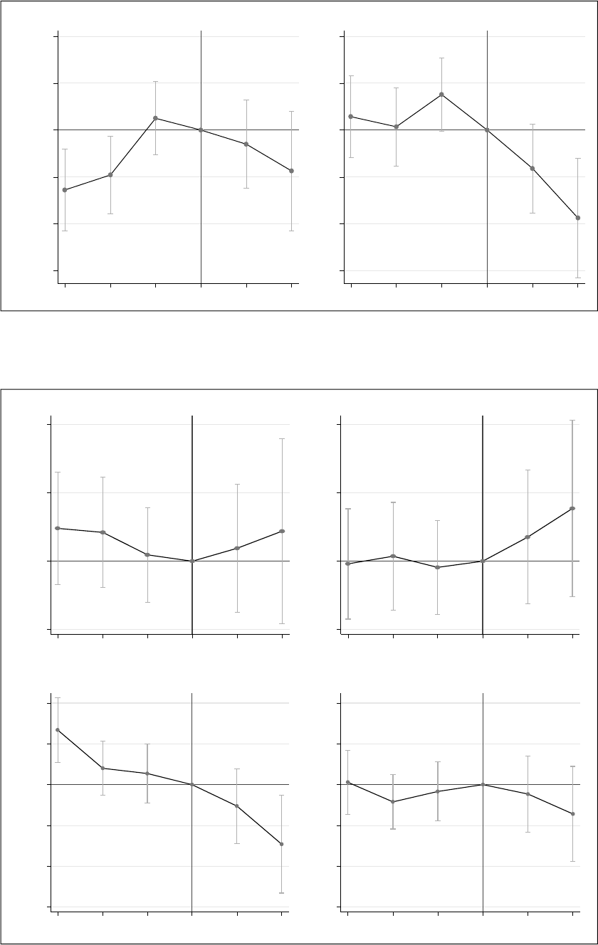
The results obtained with the exible speci‑

cations (equation 3) are presented in Figure IV,

rst with the same controls as in column 4 of

Table 3, then in a version where their (linear)

price trends before COVID are removed, i.e.

the exible version of the results presented in

column 5 of Table 3. The coefcients correspond

to the estimated gradient variations compared to

the reference period of 2019.

Figure IV – Variation in price gradients associated with distance to the centre and population density

in the municipality

A – Distance to the centre

Variation in gradient

–.05

.05

.15

2016 2017 2018 2019 2020 2021

Distance

–.05

.05

.15

2016 2017 2018 2019 2020 2021

Distance (linear trend removed)

B – Population density

Variation in gradient

–.001

–.0005

.0005

2016 2017 2018 2019 2020 2021

Density

–.001

–.0005

.0005

2016 2017 2018 2019 2020 2021

Density ((linear trend removed)

Notes: The vertical bars represent the 95% condence intervals. The rst three months of 2020 have been removed.

Sources: DVF 2016‑2021; INSEE, 2017 population census; IGN.

ECONOMIE ET STATISTIQUE / ECONOMICS AND STATISTICS N°536-37, 2022 87

COVID‑19 and Dynamics of Residential Property Markets in France: An Exploration

As the previous results suggest, even if the

coefcients estimated before the emergence

of COVID‑19 are not always signicant, we

observe a downward linear trend in the variation

of the gradient related to distance (Figure IV‑A):

before 2020, the distance‑related price gradient

was lower in absolute value in 2016 than in 2019

and appears to have increased in a fairly linear

manner between these two periods; there seems

to have been a trend towards concentration

around city centres. The year 2020 marks a clear

break and a reversal of the trend evidenced by a

decrease in the gradient in absolute value. The

presence of a trend prior to COVID‑19 would

therefore tend to cause an underestimation of

the effects of the pandemic on the distance‑

related price gradient. When the previous trend

is removed (Figure IV‑B), the effects of the

pandemic appear even more clearly.

The analysis is substantially identical with

respect to the evolution of the population density‑

related gradient. Here too, there is a clear break

in 2020: the trend towards rising prices in

densely populated municipalities compared to

less densely populated municipalities before the

emergence of COVID‑19 is followed by a clear

relative decrease in prices in densely populated

municipalities.

3.2.2. Inter‑Urban Areas Analyses

Table 4 presents the results of the estimations for

the inter‑urban areas specication (equation 2),

introducing rst the “urban areas” xed effects,

then the “urban areas×month” xed effects and,

nally, the linear trends by urban area.

In line with the predictions of the Rosen‑Roback

model, we see the positive association between

income (and therefore productivity) and property

prices. When all controls are included (column 5),

we see, after the appearance of the COVID crisis,

a relative decrease in prices in urban areas where

incomes are high, compared to urban areas

where they are lower. While urban areas that

show strong economic dynamism (measured by

household income) remain very attractive and are

therefore subject to strong demand for property,

these phenomena are less pronounced after the

appearance of COVID. This suggests a possible

inection in preferences, with urban areas with

more modest dynamics having new appeal. It

is likely that initially lower property prices will

generate greater demand, which will ultimately

contribute to higher prices in these markets.

In contrast, our results do not show price vari‑

ations following the emergence of COVID‑19

that would be explained by natural amenity

variables. The “proportion of tributaries and

rivers” variable is never signicant and the

signicant effect of the “COVID×proportion

of natural spaces” variable disappears when

linear price trends are included. The presence

of these natural amenities does not appear to

be a particularly decisive feature in the choice

of location of households after the crisis and

H4 does not seem to be empirically validated in

relation to the French property markets.

The results obtained from the exible spec‑

ications (equation 4) are shown in Figure V

(incomes) and Figure VI (natural amenities).

As for the intra‑urban area analysis, the model

is estimated rst without and then with control

of (linear) price trends before COVID, which

corresponds, respectively, to the controls of

columns 3 and 4 of Table 4.

Table 4 – Regressions at urban area level

Variables (1) (2) (3) (4)

Median income (€) 0.0110***(0.0008)

Proportion of tributaries and rivers (%) 1.1918 (0.9562)

Proportion of natural spaces (%) 0.0053 (0.0538)

COVID × Median income 0.0002 (0.0002) −0.0000 (0.0002) −0.0000 (0.0002) −0.0006**(0.0003)

COVID × Proportion of rivers and tributaries 0.2528 (0.4148) 0.0699 (0.3080) 0.0787 (0.3065) 0.5717 (0.4539)

COVID × Proportion of natural spaces −0.0248 (0.0244) −0.0704***(0.0186) −0.0662***(0.0183) −0.0019 (0.0227)

Fixed Month × Year effects Yes Yes Yes Yes

Fixed urban area effects No Yes Yes Yes

Fixed Urban area × Month effects No No Yes Yes

Urban area linear trend No No No Yes

Observations 46,976 46,976 46,973 46,973

0.2477 0.6671 0.7264 0.7352

Notes: *** p<0.01; ** p<0.05; * p<0.1. Standard errors grouped with the urban area in brackets. The estimated coefcients are multiplied by 100 to

make them easier to read. The proportion of houses in the urban area is controlled.

Reading Note: An increase in median income of €1,000 in the urban area is associated with a price increase of 11%.

Sources: DVF 2016‑2021; INSEE, 2017 population census; Corine Land Cover.

ECONOMIE ET STATISTIQUE / ECONOMICS AND STATISTICS N°536-37, 2022

Figure V – Variation in price gradients associated with income

Variation in gradient

–.0015

–.001

–.0005

.0005

.001

2016 2017 2018 2019 2020 2021

A – Income

–.0015

–.001

–.0005

.0005

.001

2016 2017 2018 2019 2020

2021

B – Income (linear trend removed)

Notes: The vertical bars represent the 95% condence intervals. The rst 3 months of 2020 have been removed.

Sources: DVF 2016‑2021; INSEE, 2017 population census.

Figure VI – Variation in price gradients associated with the proportion of rivers and tributaries

and of natural spaces in the urban area

−1

2016 2017 2018 2019 2020 2021

B – Rivers and tributaries (linear trend removed)

Variation in gradient Variation in gradient

A – Rivers and tributaries

−1

2016 2017 2018 2019 2020 2021

−.15

−.1

−.05

.05

2016 2017 2018 2019 2020 2021

C – Natural spaces

−.15

−.1

−.05

.05

D – Natural spaces (linear trend removed)

2016 2017 2018 2019 2020 2021

Notes: The vertical bars represent the 95% condence intervals. The rst 3 months of 2020 have been removed.

Sources: DVF 2016‑2021; Corine Land Cover 2018.

ECONOMIE ET STATISTIQUE / ECONOMICS AND STATISTICS N°536-37, 2022 89

COVID‑19 and Dynamics of Residential Property Markets in France: An Exploration

We rst see that the gradient positively associ‑

ating prices and incomes tended to increase in a

quite linear way until 2018, stabilised between

2018 and 2019 and decreased sharply after that

date (Figure V). Once the previous linear trend

has been removed, the gradient decrease from

2020 onwards is even sharper. This conrms the

previous results in relation to H3.

In contrast, we do not see any break in the

gradients associated with the natural amenities

of the urban area (Figure VI): the downward

trend of the gradient associated with the propor‑

tion of natural spaces continues after 2020 and

the gradient associated with the proportion of

rivers appears relatively constant throughout the

period. As suggested by the results of previous

estimations, the evolution of prices according to

the presence of these natural amenities within

the urban area does not change substantially

after the appearance of COVID.

3.3. Robustness

In the analyses conducted so far, we have exam

‑

ined the potential effects of the COVID crisis

after March 2020, i.e. the beginning of the rst

lockdown. However, the effect of COVID on

property prices is unlikely to have materialised

in the rst two months of the period, due to both

the lockdown and the delays in completing prop‑

erty transactions. Nevertheless, we estimate an

average effect over the period up to July 2021,

which does not necessarily imply that the effect

started as early as April. Moreover, prices are

unlikely to be inuenced by the inclusion or

non‑inclusion of transactions that occurred

during lockdown, as there were few such trans‑

actions: the average number of transactions per

municipality decreased by 53% in April 2020

compared to April 2019. Nonetheless, to check

the robustness of the results to the exclusion

of transactions unlikely to have been affected

by the pandemic, we re‑estimate our equations by

delaying the start of the COVID period to June

2020, which corresponds to the month following

the end of the rst lockdown. The results, which

are presented in the appendix, show that this

change of date does not change the results.

We also carry out “placebo” tests. These tests

consist in evaluating the effect of ctitious

pandemics that would have occurred in 2017,

2018 and 2019 and considering only transactions

that occurred before 2020. The idea is that these

ctitious pandemics should not have a signicant

effect on price dynamics. We estimate the same

specications as those presented in column 5

of Table 3 for municipalities, and column 4 of

Table 4 for urban areas, varying the start date

of the pandemic between 2017 and 2019. The

results (see Appendix) show – reassuringly – no

signicant change at the 5% threshold in price

dynamics after these ctitious pandemics.

* *

In this article, we have sought to explore how

the pandemic has affected household location

choices and residential property markets in

France. The results show that, at the intra‑urban

area level, prices increased relatively more in

the least densely populated areas as well as in the

areas located farthest from urban centres after

the emergence of COVID‑19, suggesting that

households are seeking more space and place

less value on the positive externalities that can

be produced by a high population density. At the

inter‑urban areas level, the level of productivity,

reected by the level of income, also partly

explains the differences in price variations. In

contrast, we do not nd any signicant effect

related to the level of amenities.

Our results therefore support the expectations

of hypotheses 1 and 2, according to which

property prices decrease in the centre and

increase in the periphery of urban areas, where

population densities are lower. They join the

results of Gupta et al. (2021) and Ramani &

Bloom (2021) based on American data. The

former show that the crisis has indeed led to

lower property prices and rents in city centres

and higher prices in areas away from the centre

(attening this relationship between distance to

the centre and prices in most US metropolitan

areas). The latter show, in major American

cities, a shift (the “donut effect”) in household

demand for property from densely populated

city centres towards more sparsely populated

suburban locations.

Our estimates also support hypothesis 3,

according to which prices rise in agglomerations

with low productivity. This result is in line with

those obtained by Brueckner et al. (2021) which

show, on the basis of US data, downward pres‑

sure on property prices in high‑productivity cities

following the health crisis and the development

of working remotely. In contrast, hypothesis 4,

according to which prices would tend to increase

in agglomerations with a certain level of natural

amenities, is not veried in our estimates. On

this point, our results therefore differ from those

obtained by Brueckner et al. (2021) showing that

property prices have increased in cities with high

ECONOMIE ET STATISTIQUE / ECONOMICS AND STATISTICS N°536-37, 2022

levels of amenities and decreased in cities with

low levels of amenities. However, for natural

amenities, the authors use a richer set of indi‑

cators (differences in temperature, precipitation,

proximity to the oceans, etc.), some of these not

being available at the level of analysis carried

out here. We therefore cannot rule out that the

amenities that we take into consideration are not

necessarily those for which the value placed on

them has changed the most.

Our exploration also has other limitations that

we must emphasise. In particular, we consid‑

ered that the pandemic was able to affect the

demand for property mainly through two factors:

the increased use of telework and changes in

preferences related to successive lockdowns.

This allowed us to identify a limited number of

hypotheses that could then be tested. However,

this does not exclude other effects that the

pandemic may have had on behaviour related to

demand for property: for example, fear of conta‑

gion may have increased the psychological costs

of transport. In this case, households would opt

for locations close to the centre or would give

preference to the use of a private vehicle, with an

additional cost. This could then mitigate changes

in the price gradient across the urban space. It is

also not possible for us to distinguish between

the respective effects of the two potential factors,

or to say that they are precisely the ones that

explain the observed evolutions of prices.

Deeper societal changes, particularly in relation

to work‑life balance, may contribute to some

of the changes just as much as changes directly

caused by the crisis. If this is the case, the health

crisis may have acted as an accelerator, leading

households to concretise mobility projects they

already considered before COVID.

Keeping these limitations in mind, it would

nevertheless seem that, at intra‑urban area

level, we are witnessing a strengthening of

the phenomenon of peri‑urbanisation that has

already been under way for several decades. The

effect observed on the prices of the residential

property markets of distant and sparsely popu‑

lated municipalities suggests that it is primarily

individuals who can work remotely, who are

often executives and have strong economic and

cultural capital, that have ocked to peri‑urban

municipalities. Therefore, in addition to an

effect on property prices, these potential changes

in the social composition of the inhabitants can

ultimately have consequences on the overall

economic dynamics of the municipalities.

This can lead to gentrication processes, with

increased inequality and greater exclusion of

the most fragile social categories. Nevertheless,

if relatively wealthy populations arrive in

municipalities where less afuent populations

can remain despite rising price dynamics, for

example through social housing, this could

foster social diversity.

At inter‑urban areas level, the fact that property

prices in cities with the lowest productivity

are catching up suggests a broader economic

and social rebalancing: territories that could

have been losing economic impetus could be

revitalised by the arrival of a new population.

Nevertheless, at this stage, our analysis does

not allow us to observe the effects of a social

recomposition of municipalities or urban areas

at granular level. In addition, it is difcult to

determine whether the changes observed over

the study period will be conrmed in the longer

term or whether they are only temporary: our

data stopped in July 2021, at a time when the

pandemic was not over and government recom‑

mendations on working remotely were still

in place. It is therefore necessary to question

whether the changes observed will last beyond

the pandemic and whether they will affect the

dynamics of socio‑spatial inequalities.

BIBLIOGRAPHY

Ahlfeldt, G., Roth, D. & Seidel, T. (2018). The Regional Effects of Germany’s National Minimum Wage.

Economics Letters, 172, 127–130. https://doi.org/10.1016/j.econlet.2018.08.032

Angrist, J. & Pischke, J. (2008). Mostly Harmless Econometrics. Princeton University Press.

Alonso, W. (1964). Location and Land Use. Toward a General Theory of Land Rent. Cambridge: Harvard

University Press.

Bergeaud, A., Eyméoud, J.‑B., Garcia, T. & Henricot, D. (2022). Working From Home and Corporate Real

Estate. LIEPP Working Paper. https://hal‑sciencespo.archives‑ouvertes.fr/hal‑03548889

Brajon, D. & Leroi, P. (2022). Le télétravail s’installe durablement. L’Institut Paris Région, Note rapide

N° 930. https://www.institutparisregion.fr/leadmin/NewEtudes/000pack2/Etude_2728/NR_930_web.pdf

ECONOMIE ET STATISTIQUE / ECONOMICS AND STATISTICS N°536-37, 2022 91

COVID‑19 and Dynamics of Residential Property Markets in France: An Exploration

Breuillé, M., Le Gallo, J., & Verlhiac, A. (2022). Residential Migration and the COVID‑19 Crisis: Towards

an Urban Exodus in France? Economie & Statistique / Economics and Statistics, 536‑37, 57–73 (ce numéro).

Bricongne, J.‑C., Meunier, B. & Pouget, S. (2021). Web Scraping Housing Prices in Real‑time: the Covid‑19

Crisis in the UK. Banque de France, Working Paper N° 827. http://dx.doi.org/10.2139/ssrn.3916196

Brueckner, J., Kahn, M. & Lin, G. (2021). A New Spatial Hedonic Equilibrium in the Emerging

Work‑from‑Home Economy. NBER Working Paper N° 28526. https://doi.org/10.3386/w28526

Cheung, K., Yiu, E. & Xiong, C. (2021). Housing Market in the Time of Pandemic: A Price Gradient Analysis

from the COVID‑19 Epicentre in China. Journal of Risk and Financial Management, 14(3), 1–17.

https://doi.org/10.3390/jrfm14030108

Duc, C. & Souquet, C. (2020). L’impact de la crise sanitaire sur l’organisation et l’activité des sociétés. Insee

Première N° 1830, décembre. https://www.insee.fr/fr/statistiques/4994488

Dustmann, C., Lindner, A., Schönberg, U., Umkehrer, M. & vom Berge, P. (2022). Reallocation Effects of

the Minimum Wage. Quarterly Journal of Economics, 137(1), 267–328. https://doi.org/10.1093/qje/qjab028

Egami, N. & Yamauchi, S. (2021). Using Multiple Pre‑treatment Periods to Improve Difference‑in‑

Differences and Staggered Adoption Designs. Working Paper. https://doi.org/10.48550/arXiv.2102.09948

France Stratégie (2022). Les villes moyennes, un pilier durable de l’aménagement du territoire ? La note

d’analyse, janvier 2022. https://www.strategie.gouv.fr/sites/strategie.gouv.fr/les/atoms/les/fs‑2022‑na107‑

villes‑moyennes‑janvier.pdf

Gupta, A., Mittal, V., Peters, J. & Van Nieuwerburgh, S. (2022). Flattening the Curve: Pandemic Induced

Revaluation of Urban Real Estate. Journal of Financial Economics, 146(2), 594–636.

https://doi.org/10.1016/j.jneco.2021.10.008

Huang, N., Pang, J. & Yang, Y. (2021). COVID‑19 and the Urban Housing Market in China. Working Paper

SSRN. http://dx.doi.org/10.2139/ssrn.3642444

Liu, S. & Su, Y. (2021). The Impact of the COVID‑19 Pandemic on the Demand for Density: Evidence from

the U.S. Housing Market. Economics Letters, 207, 110010. https://doi.org/10.1016/j.econlet.2021.110010

McFadden, D. (1977). Modeling the Choice of Residential Location. Transportation Research Record.

https://onlinepubs.trb.org/Onlinepubs/trr/1978/673/673‑012.pdf

Mills, E. S. (1967). An Aggregative Model of Resource Allocation in a Metropolitan Area. American Economic

Review, 57, 97–210. https://www.jstor.org/stable/1821621

Monras, J. (2019). Minimum Wages and Spatial Equilibrium: Theory and Evidence. Journal of Labor

Economics, 37(3), 853–904. https://doi.org/10.1086/702650

Mora, R. & Reggio, I. (2019). Alternative Diff‑in‑Diffs Estimators with Several Pretreatment Periods.

Econometric Reviews, 38(5), 465–486. https://doi.org/10.1080/07474938.2017.1348683

Muth, R. F. (1969). Cities and Housing. The Spatial Pattern of Urban Residential Land Use. Chicago and

London: The University of Chicago Press.

Qian, X., Qiu, S., Zhang, G. (2021). The impact of COVID‑19 on housing price: Evidence from China.

Finance Research Letter, 43, 101944. https://doi.org/10.1016/j.frl.2021.101944

Ramani, A. & Bloom, N. (2021). The Donut Effect of Covid‑19 on Cities. NBER Working Paper N° 28876.

https://doi.org/10.3386/w28876

Roback, J. (1982). Wages, Rents, and the Quality of Life. Journal of Political Economy, 90(6), 1257–1278.

https://www.jstor.org/stable/1830947

Rosen, K. T. (1979). A Regional Model of Multifamily Housing Starts. Real Estate Economics, 7, 63–76.

https://doi.org/10.1111/1540‑6229.00195

ECONOMIE ET STATISTIQUE / ECONOMICS AND STATISTICS N°536-37, 2022

APPENDIX

____________________________________________________________________________________________

ROBUSTNESS ANALYSES

Table A1 – Regression at municipality level (start June 2020)

Variables (1) (2) (4) (5) (6)

Population density 0.0016***

(0.0003)

Distance to the UA centre −1.1553***

(0.0326)

COVID × Population density −0.0004*** −0.0004*** −0.0002** −0.0002** −0.0005***

(0.0001) (0.0001) (0.0001) (0.0001) (0.0001)

COVID × Distance to the UA centre 0.0093 0.0062 0.0337** 0.0434*** 0.0699***

(0.0133) (0.0125) (0.0164) (0.0168) (0.0236)

Fixed Month × Year effects Yes Yes Yes Yes Yes

Fixed municipality effects No Yes Yes Yes Yes

Date × Urban area No No Yes Yes Yes

Month × Municipality No No No Yes Yes

Municipality linear trend No No No No Yes

Observations 193,173 193,162 193,162 187,031 187,031

0.2255 0.5083 0.5121 0.6352 0.6522

Notes: *** p<0.01; ** p<0.05; * p<0.1. Standard errors grouped with the municipality in brackets. The estimated coefcients are multiplied by 100

to make them easier to read. The proportion of houses in the municipality is controlled.

Sources: DVF 2016‑2021; INSEE, 2017 population census.

Table A2 – Regression at urban area level (start June 2020)

Variables (1) (2) (3) (4)

Median income (€) 0.0111***(0.0008)

Proportion of tributaries and rivers (%) 1.2033 (0.9582)

Proportion of natural spaces (%) 0.0041 (0.0538)

COVID × Median income −0.0001 (0.0003) −0.0002 (0.0002) −0.0002 (0.0002) −0.0009***(0.0003)

COVID × Proportion of tributaries and rivers 0.2292 (0.4689) 0.1459 (0.3552) 0.2183 (0.3590) 0.7554 (0.4792)

COVID × Proportion of natural spaces −0.0216 (0.0263) −0.0768***(0.0200) −0.0757***(0.0198) −0.0192 (0.0236)

Fixed Month × Year effects Yes Yes Yes Yes

Fixed urban area effects No Yes Yes Yes

Fixed Urban area × Month effects No No Yes Yes

Urban area linear trend No No No Yes

Observations 46,976 46,976 46,973 46,973

0.2477 0.6671 0.7264 0.7353

Notes: *** p<0.01; ** p<0.05; * p<0.1. Standard errors grouped with the urban area in brackets. The estimated coefcients are multiplied by 100 to

make them easier to read. The proportion of houses in the urban area is controlled.

Sources: DVF 2016‑2021; INSEE, 2017 population census; Corine Land Cover.

ECONOMIE ET STATISTIQUE / ECONOMICS AND STATISTICS N°536-37, 2022 93

COVID‑19 and Dynamics of Residential Property Markets in France: An Exploration

Table A3 – Placebo tests

Municipalities

2019 2018 2017

Period × Population density −0.0001 (0.0001) −0.0002 (0.0002) 0.0002(0.0001)

Period × Distance to the centre −0.0364 (0.0283) 0.0268(0.0343) 0.0184(0.0282)

Observations 136,607 136,607 136,607

0.6862 0.6862 0.6862

Urban areas

2019 2018 2017

Period × Median income −0.0004 (0.0003) 0.0006*(0.0003) 0.0000(0.0003)

Period × Proportion of rivers and tributaries (%) 0.0602 (0.4041) −0.2532 (0.5066) 0.1060(0.4426)

Period × Proportion of natural spaces (%) 0.0185(0.0256) 0.0250 (0.0288) −0.0353 (0.0238)

Observations 34,937 34,937 34,937

0.7649 0.7649 0.7649

Notes: *** p<0.01; ** p<0.05; * p<0.1. Standard errors grouped with the municipality for municipality level estimates and with the urban area for

urban area level estimates, in brackets. The estimated coefcients are multiplied by 100 to make them easier to interpret. The control variables

correspond to those in column (4) of Table 3 (or 4) for estimates at municipality (urban area) level. Transactions after 31 December 2019 are

removed. The “period” variable corresponds to a ctitious processing date starting at the beginning of the year, indicated at the top of each column.

Sources: DVF 2016‑2021; INSEE, 2017 population census; Corine Land Cover.