Excel Basic Uses for Excel Menu Organization

Excel Basic

Uses for Excel

-Number Crunching

-Creating Charts and Tables

-Organizing Lists and Data

Menu Organization

Excel 2010 uses tabs and ribbons to organize the menu options.

Many of the same functions you are used to seeing in Microsoft Word are also present in Excel. At the top of

the screen you’ll notice the ribbons for “File”, “Home,” and “Insert”. You can switch between ribbons to do

different things.

Layout and Cells

An Excel spreadsheet is a grid of “cells” and is organized into rows and columns. The rows are arranged in

number order, and columns are assigned letters. Each cell has a unique “cell reference” – a way to identify

that cell. Cell references are simply where the columns and rows meet.

Here the currently selected or “active” cell is C5. The black borders show you which cell is the active cell, and

the name box in the top left corner displays the cell reference of that cell.

Navigating and Entering Data

There are a number of ways to navigate your spreadsheet. You can use the mouse and single click the cell

you’d like to work in. You can also use the “tab” key to advance the active cell one column to the right. You

can use the “enter” key to advance the active cell one row down. You can also use the direction keys to move

your active cell around your spreadsheet.

To enter data into Excel select the cell where you’d like to enter information and begin typing. If you prefer,

you can also select the cell where you’d like to enter data and then type it into the formula bar at the top of

the screen, though this is mostly used for formulas. Note that if you want to edit the information in a cell you

have to double click that cell, because if you single click on a cell that’s already filled and begin typing you will

instead replace what is already in there.

Worksheets

As you use Excel you may wish to separate your data into multiple worksheets. Worksheets are like

separate pages in a notebook. You have tabs at the bottom of your screen that will allow you to navigate

between worksheets. By default you will be given 3 worksheets (labeled 1, 2, and 3).

You can add, delete, rename, move, copy, color-code, etc. your worksheets by right-clicking on the tab you

wish to edit. That will bring up a small menu with all your tab options.

You can zoom in or out of your spreadsheet using the slider control in the lower right of the spreadsheet.

Selecting Cells, Rows, and Columns

Highlighting is an important skill that is used frequently in Excel worksheets. Highlighting in Excel works the

same way as highlighting in Word, PowerPoint, or other Microsoft products. To highlight in Excel, you click

and drag in order to select a given cell and/or area.

You can also highlight entire rows or columns. Do that by clicking on either the column letter or row number.

Select multiple columns by clicking and dragging across multiple column letters or by holding down “Shift” and

selecting the first and last column in your desired range.

Holding down “Ctrl” allows you to select noncontiguous columns, rows, or cells.

Formatting Font and Alignment

The tools for changing the formatting of your worksheet can be found on the Home ribbon. If you are familiar

with Microsoft Word 2010, you will recognize many of the same options, plus some additional features unique

to Excel 2010.

Some of the available formatting options are font style, font size, bold, underline, fill color, letter color, and

cell borders. You can also adjust the position of text within the cells, centering data vertically or horizontally,

left justifying, right justifying, wrapping text, etc. In this example, the heading row has been selected and

various formatting changes have been applied:

Cell Formatting

If the data you enter is too long for the cell, you can use the mouse to alter the width of your columns or the

height of your rows to accommodate the text. To change the width of a cell, place your mouse pointer on the

division between the column letters, click and drag the cell until the width is acceptable. Another option is to

double click on the division between the two columns. This will auto fit the column to fit the text.

Wrapping Text

Text Wrapping allows you to fit all of your text in one cell. By default, text in Excel that is longer than the cell

will overlap into the cells next to it, truncating the text. Wrapping tells Excel that instead of going into the next

column, wrap the text around within the cell (making the row height increase.)

Start by selecting the cell(s) you wish to edit. In this example, select Row 3. Then, click “Wrap Text.”

The column headings now all fit within the width of their cells.

Merge and Center

In addition to centering data within a cell, Excel 2010 also allows you to center text across multiple columns

using the Merge & Center option. This is ideal for centering a heading across a spreadsheet.

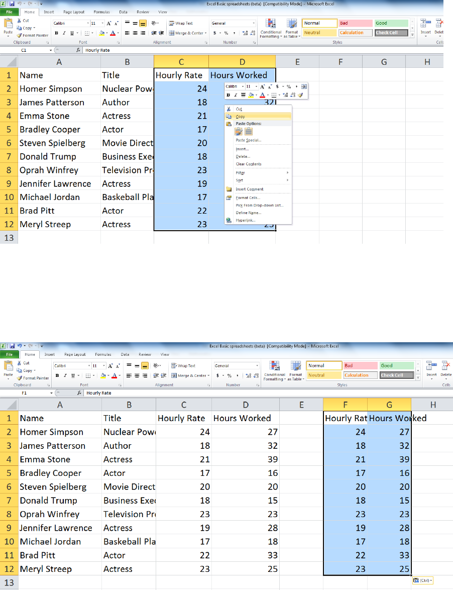
Copying and Pasting

Copying and pasting data in Excel 2010 is a lot like copying and pasting in other Microsoft programs. Right click

on the cell you wish to copy and paste and select “Copy.” Select the cell you wish to paste to, then right click

to view your paste and “paste special” options.

In most cases the regular paste option will work just fine. You can also copy and paste by using the Ctrl-C and

Ctrl-V shortcuts. Ctrl-C executes a copy command, and Ctrl-V executes a paste command. You can also cut and

paste instead of copying and pasting. This will move whatever you cut to the designated location instead of

creating another copy of it there. The shortcut for the “Cut” command is Ctrl-X.

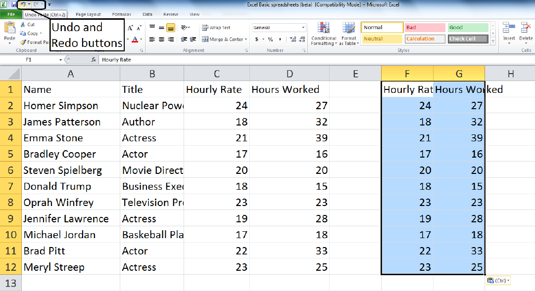
Undo and Redo

One useful Excel feature that you may find yourself using a lot is the “Undo” command. If you accidentally

make a change to your worksheet or enter something that you decide you don’t want, you can click the

counterclockwise arrow button at the top left of your screen to rewind your latest action. The shortcut for this

is Ctrl-Z.

If you undo something and decide that you liked it better the way before, you can cancel the undo by clicking

the clockwise arrow Redo button next to the Undo button. The shortcut for Redo is Ctrl-Y.

Adding and Deleting Columns and Rows

Adding or Deleting columns and rows to your spreadsheet is easy. To add a column: click the heading of

the column to the right (or row below) of where you want to insert a new column. Right-click the selected

column and click insert.

To delete a column or row, select the column or row, right-click, and select delete. Note: using the

“Delete” key on the keyboard will only delete the row or column’s contents, not the row or column

itself.

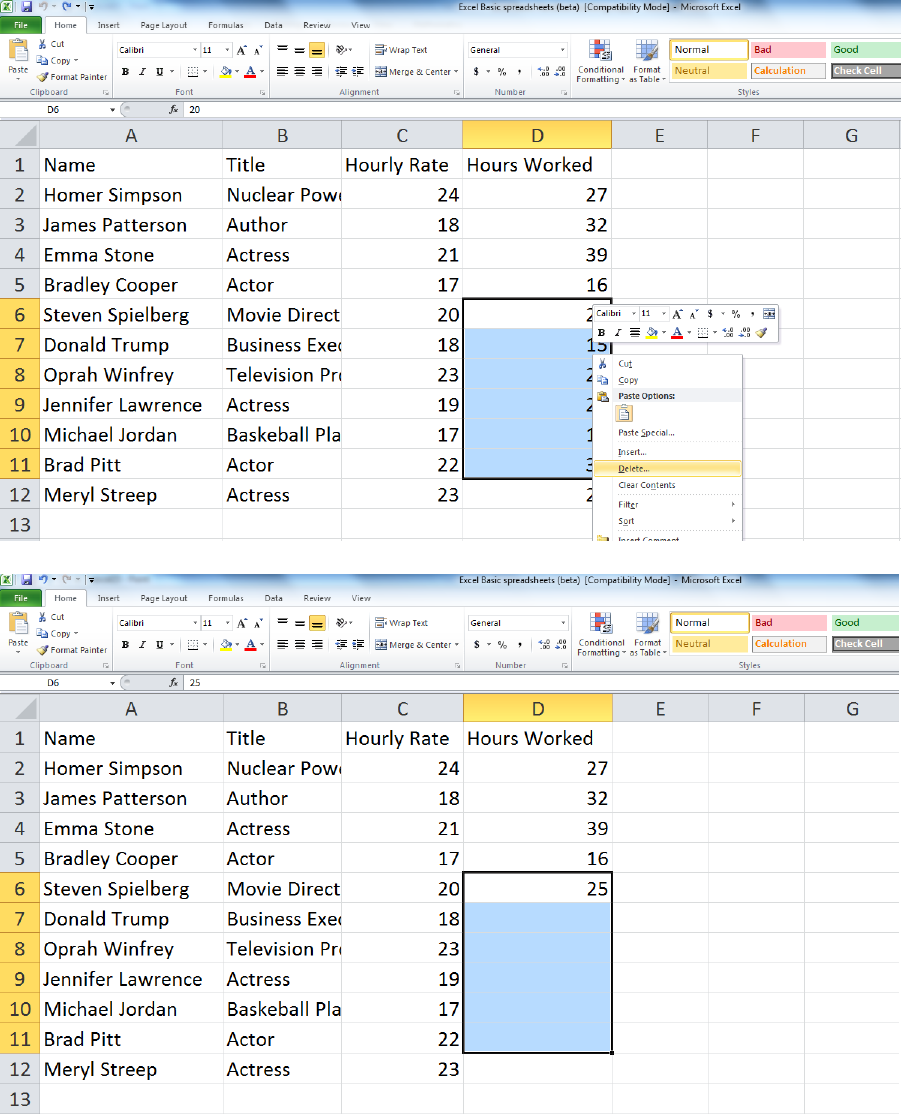
Deleting Cells and Data

Deleting cells and data can sometimes be tricky. Pay attention to the options carefully and remember to use

your undo button if you need to!

To delete just the data in the cells (not the cells themselves) click the cells or range you want to delete.

Pressing the “Delete” key will erase the data in the cells. Or, you can highlight the cells you want to delete,

right click with your mouse and choose” Clear Contents.” Both methods will only remove the data in the cells.

You can also delete the highlighted cells themselves by right clicking on them and clicking “delete.” This will

ask you how you want to fill in the empty space. In this example we are shifting the cells below the cells we

deleted to where the highlighted cells were located before.

Copying a Spreadsheet

After spending a considerable amount of time creating and adjusting your spreadsheet, you might find it

useful to copy the completed spreadsheet to another tab or workbook so that you do not have to recreate it

from scratch the next time you need to make a similar spreadsheet. Right click the bottom tab of your

spreadsheet and click “Move or Copy”

You can move your spreadsheet to another workbook or simply to another tab in your current workbook.

Don’t forget to check “Create a copy.”

Click OK and you will notice that an exact duplicate has been created. Now you can use the duplicate

spreadsheet as a template for a new spreadsheet.

Hiding and Unhiding Columns or Rows

If you have a large spreadsheet that has a lot of rows and columns of data, sometimes it is helpful to

temporarily hide the rows or columns that you are not using at the moment. To hide a column, for instance,

you can select the letter at the top of the column, right click, and select “Hide.”

In this example, column E has been hidden. In its place, you will see a dark black vertical line reminding you

that information is hidden.

When you wish to unhide the column, simply highlight the columns on either side of the hidden column, right

click, and select “Unhide.”

The hidden column is now visible.

Freezing Columns or Rows

You can freeze a portion of your spreadsheet, such as your headings, so that if you scroll down or to the right

your column and row headings will remain visible at all times.

Formulas

Formulas are what you use to perform calculations within your Excel spreadsheets.

Formula Structure:

Excel formulas work a little differently than you may be used to. Usually, you’d expect to see a formula that

looks like this: 2+2=4. When using Excel, the “=” always comes first. This is your way of telling Excel that you

are using a formula and not just typing text. Anything after the “=” is recognized as part of the formula. You

always type your formula in the cell you want your answer to be in.

Mathematical Operators:

+ Addition

- Subtraction

* Multiplication

/ Division

Referencing Cells:

Although you can enter specific values in your Excel formulas, you can also easily reference data in specific

cells. So, instead of your equation being =2+2, it could read =A1+B1. It is often preferable to use cell

references instead of numbers so that if you have to go back and change the numbers in your data set, your

formulas will automatically adjust to the change.

In our spreadsheet, if you wanted to find the answer to “Total” for column B or “Morning” this is what your

formula would look like: =B4+B5+B6+B7+B8+B9+B10+B11+B12+B13+B14

Basic Functions

Function Elements:

Because functions are a type of formula, they must also start with an “=”.

Functions are different in that they each have a name. For example, the name of the function for addition is

“sum.” You can type functions directly into your worksheet or you can use the Insert Function dialogue box to

help you construct functions.

Structure:

Functions use arguments to indicate the cell addresses you want the function to calculate. The arguments

(cell references or cell addresses) are contained in parentheses. You can use commas to separate the

arguments, or you can use a range.

Using a Range:

A range is an easier way of entering a series of cell addresses into a formula. Let’s demonstrate using a range

by finding the total for column C:

-Start with “=”

-Since we are adding the column, we need the function for addition, which is “sum”. Type “sum” after your

“=”.

-Open your parentheses.

-Enter your range. You could enter the references individually separated by a comma, but using a range is an

easier way to include your references. Start with C4. Click and drag your mouse pointer from C4 all the way to

C14. Take a look at your function. Excel should’ve inserted “C4:C14”. That is a range. The range starts with C4

and ends with C14. The “:” in between should be read as “through.” Thus, this forms an equation that says:

“EXCEL…add C4 through C14.”

-Don’t forget to close your parentheses!

AutoFunctions

Excel makes using functions even easier with automatic functions. AutoFuctions do all the work for you!

You can use AutoFunctions for many different functions in Excel (AutoMinimum, AutoMaximum, AutoAverage,

etc.)

This is what your finished spreadsheet should look like:

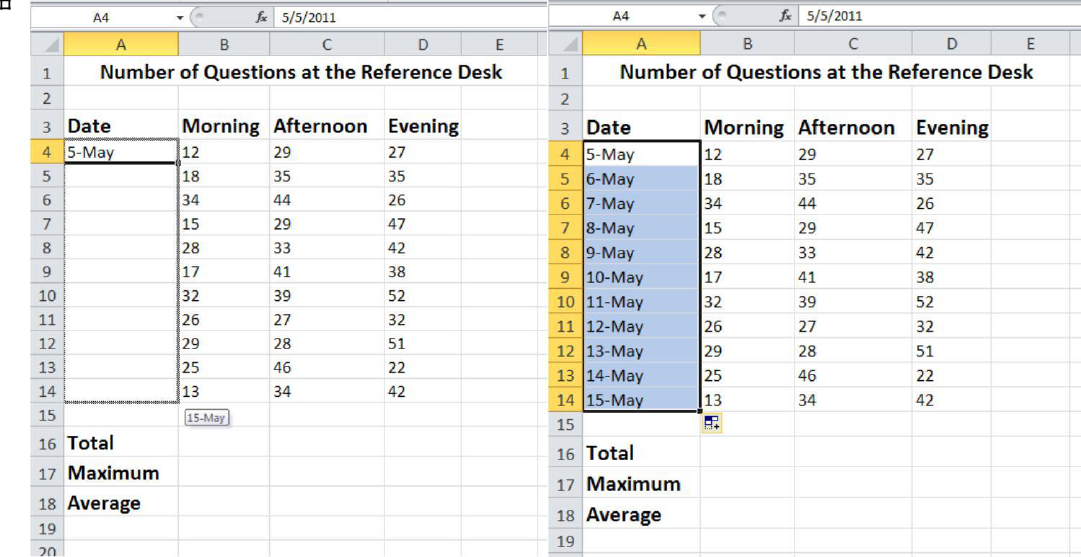
AutoFill

When you make a cell active in the worksheet a small fill handle appears in the lower-right corner of the cell.

You can use the fill handle to create an AutoFill series. This will work with text, dates, numbers, years, and

other types of data.

AutoFill the dates in this spreadsheet by placing your mouse pointer over the small square located in the

bottom-right of the active cell. Your pointer will turn into a black plus sign when you’ve placed it properly.

Double click or click and hold your left mouse button and drag downwards as Excel fills in your dates.

Once Excel has AutoFilled the dates, you will notice there is now a smart tag with additional AutoFill options.

This will allow you to change what Excel displays (maybe you wanted the dates listed by months instead of

days, for example).

If you start with the first few numbers in a number sequence, AutoFill can finish the sequence so that you

don’t have to fill out the rest of it. You can also use AutoFill to quickly copy a piece of data to multiple cells by

selecting the cell you wish to copy and dragging it down. Likewise, you can quickly copy a formula to multiple

cells.

Relative Cell References vs. Absolute Cell References

When Excel performs the AutoFill function, it will by default adjust the cell references in the formula as it

moves down each row of data calculations:

Notice that after AutoFilling the Salary Owed column, the cell references in each number’s formula changes to

correctly reflect the different rows. Because the cell references in each number’s formula changes, these are

called “relative cell references.”

Sometimes, however, you will want all formulas in a column to refer to a fixed number; such is the case when

calculating taxes, since the same tax rate applies to each row. By referring to this fixed number, you can easily

change the tax rate later and have the change automatically apply to the entire column without having to

make changes to each formula.

In this example, an absolute cell reference has been created for the tax rate in cell B14. In creating the first

formula in column F, dollar signs ($) have been placed in front of the column letter and row number of the

absolute cell reference. These dollar signs tell Excel to reference the exact same cell for the tax rate when

AutoFilling the rest of the column.

If you want to change the tax rate in the future, changing the tax rate number in cell B14 will now

automatically apply the change to all formulas in column F.

Copying Formulas

Be careful when copying and pasting formulas. If you copy one or more formulas and then right click on a cell

to paste the formulas (without using the Ctrl-V shortcut), you will see options besides a standard paste such as

paste values, paste formulas, and transposed paste. If you select paste values, this will only copy the values

that result from your original formulas instead of the formulas themselves. If you instead copy and paste

formulas, you may have to adjust the cell references in the formulas so that they are pointing at the right cells.

Formatting Numbers

Since Excel is designed for number crunching, it is frequently necessary to format numbers in order to tell

Excel whether you are dealing with currency, percentages, decimals, whole numbers, etc. These, plus other

number formatting options, can also be found on the Home ribbon.

In this example the tax rate of 0.25 was highlighted, then the % button was selected on the ribbon, converting

the decimal to a percentage. You can also change the formatting by selecting the cell, right clicking the mouse,

selecting the number category you want, and, if needed, adjust the number of decimal places. Click OK.

These same methods can be used to apply other changes to the numbers on your spreadsheet. In this example

pay rates, salaries, and taxes have been formatted to include dollar signs and two decimal places per number.

You will notice that right clicking and selecting the formatting menu allows you to adjust the decimal places

and also gives you options for choosing how you want negative numbers to appear: with a negative symbol, in

parentheses, in red, etc.

Charts and Graphs

Making charts and graphs from Excel data is easy. Highlight the data you wish to include in your graph. Click

on the “Insert” ribbon, then choose from a wide variety of chart types and sub-types. Not all chart types work

for all types of data but it’s very easy to switch between different types of charts until you find the one that

works the best.

Protecting Your Spreadsheet

Protecting your Excel spreadsheets is a good idea if multiple people have access to the spreadsheet. You can

protect a single worksheet or an entire workbook. Choose the Review Ribbon and you will then see the

“Protect” options.

When you place protection on a spreadsheet or workbook you are making sure no data can be changed. You

will need to create a password to turn off the protection. Make sure to remember your password because

there is no way to look it up. To remove the protection, make sure you are in the Review Ribbon, click

“Unprotect Sheet” and enter your password.

Printing Options

Choosing the Page Layout ribbon allows you to set up how you would like your spreadsheet to look when you

print it.

You can also select the paper size, set page breaks, and set a background color or image.

The ”Sheet Options” can also be helpful when printing. You can choose to print the gridlines and headings

(the column letters and row numbers) by checking the boxes for printing.