

An agency of the
European Union
Authors
EASA
Jean Marc Cluzeau
Xavier Henriquel
Georges Rebender
Guillaume Soudain
Daedalean AG
Dr. Luuk van Dijk
Dr. Alexey Gronskiy
David Haber
Dr. Corentin Perret-Gentil
Ruben Polak
Disclaimer
This document and all information contained or referred to herein are provided for information
purposes only, in the context of, and subject to all terms, conditions and limitations expressed in
the IPC contract P-EASA.IPC.004 of June 4th, 2019, under which the work and/or discussions
to which they relate was/were conducted. Information or opinions expressed or referred to
herein shall not constitute any binding advice nor they shall they create or be understood as
creating any expectations with respect to any future certification or approval whatsoever.
All intellectual property rights in this document shall remain at all times strictly and exclusively
vested with Daedalean. Any communication or reproduction in full or in part of this document
or any information contained herein shall require Daedalean’s prior approval and bear the full
text of this disclaimer.

An agency of the
European Union
Contents
1 Executive summary 5
A note about this document . . . . . . . . . . . . . . . . . . . . . . . . . . . . . . 6
2 Introduction 7
2.1 Background . . . . . . . . . . . . . . . . . . . . . . . . . . . . . . . . . . . . 7
2.2 Learning Assurance process elements . . . . . . . . . . . . . . . . . . . . . . . 8
2.3 Other key takeaways from the IPC . . . . . . . . . . . . . . . . . . . . . . . . 8
2.4 Aim of the report . . . . . . . . . . . . . . . . . . . . . . . . . . . . . . . . . 9
2.5 Outline of the report . . . . . . . . . . . . . . . . . . . . . . . . . . . . . . . 9
2.6 Terminology . . . . . . . . . . . . . . . . . . . . . . . . . . . . . . . . . . . . 10
3 Existing guidelines, standards and regulations, and their applicability to machine
learning-based systems 12
3.1 EASA AI Roadmap . . . . . . . . . . . . . . . . . . . . . . . . . . . . . . . . 12
3.2 EU guidelines for trustworthy AI . . . . . . . . . . . . . . . . . . . . . . . . . 13
3.3 Existing guidelines and standards . . . . . . . . . . . . . . . . . . . . . . . . . 16
3.4 Other documents and working groups . . . . . . . . . . . . . . . . . . . . . . 18
3.5 Comparison of traditional software and machine learning-based systems . . . . 20
4 Use case definition and Concepts of Operations (ConOps) 22
4.1 Use case and ConOps . . . . . . . . . . . . . . . . . . . . . . . . . . . . . . . 22
4.2 System description . . . . . . . . . . . . . . . . . . . . . . . . . . . . . . . . 24
4.3 Notes on model training . . . . . . . . . . . . . . . . . . . . . . . . . . . . . 26
4.4 Selection criteria . . . . . . . . . . . . . . . . . . . . . . . . . . . . . . . . . 27
5 Learning process 28
5.1 What is a learning algorithm? . . . . . . . . . . . . . . . . . . . . . . . . . . . 28
5.2 Training, validation, testing, and out-of-sample errors . . . . . . . . . . . . . . 30
5.3 Generalizability . . . . . . . . . . . . . . . . . . . . . . . . . . . . . . . . . . 32
6 Learning Assurance 43
6.1 Learning Assurance process overview . . . . . . . . . . . . . . . . . . . . . . . 43
6.2 Dataset management and verification . . . . . . . . . . . . . . . . . . . . . . 45
6.3 Training phase verification . . . . . . . . . . . . . . . . . . . . . . . . . . . . 51
3

An agency of the
European Union
Daedalean – EASA CoDANN IPC Extract 4
6.4 Machine learning model verification . . . . . . . . . . . . . . . . . . . . . . . 53
6.5 Inference stage verification . . . . . . . . . . . . . . . . . . . . . . . . . . . . 57
6.6 Runtime monitoring . . . . . . . . . . . . . . . . . . . . . . . . . . . . . . . . 57
6.7 Learning Assurance artifacts . . . . . . . . . . . . . . . . . . . . . . . . . . . 62
7 Advanced concepts for Learning Assurance 63
7.1 Transfer learning . . . . . . . . . . . . . . . . . . . . . . . . . . . . . . . . . 63
7.2 Synthesized data . . . . . . . . . . . . . . . . . . . . . . . . . . . . . . . . . 66
8 Performance assessment 70
8.1 Metrics . . . . . . . . . . . . . . . . . . . . . . . . . . . . . . . . . . . . . . 70
8.2 Model evaluation . . . . . . . . . . . . . . . . . . . . . . . . . . . . . . . . . 75
9 Safety Assessment 77
9.1 Safety Assessment process . . . . . . . . . . . . . . . . . . . . . . . . . . . . 77
9.2 Functional Hazard Assessment . . . . . . . . . . . . . . . . . . . . . . . . . . 78
9.3 DAL Assignment . . . . . . . . . . . . . . . . . . . . . . . . . . . . . . . . . 85
9.4 Common Mode Analysis . . . . . . . . . . . . . . . . . . . . . . . . . . . . . 86
9.5 Neural network Failure Mode and Effect Analysis (FMEA) . . . . . . . . . . . 86
10 Use case: Learning Assurance 88
11 Conclusion & future work 89
References 91
Notations 100
Index 101
Acronyms 103

An agency of the
European Union
Chapter 1
Executive summary
This is a public extract of the report that resulted from the collaboration between EASA and
Daedalean in the frame of an Innovation Partnership Contract (IPC) signed by the Agency.
The project ran from June 2019 to February 2020.
The project titled “Concepts of Design Assurance for Neural Networks” (CoDANN) aimed
at examining the challenges posed by the use of neural networks in aviation, in the broader
context of allowing machine learning and more generally artificial intelligence on-board aircraft
for safety-critical applications.
Focus was put on the “Learning Assurance” building-block of the EASA AI Roadmap 1.0
[EAS20] which resulted in significant progress on three essential aspects of the “Learning
Assurance” concept:
1. The definition of the W-shaped Learning Assurance life-cycle as a foundation for future
guidance from EASA for machine learning / deep learning (ML/DL) applications. It
provides an outline of the essential steps for Learning Assurance and their connection
with traditional Development Assurance processes.
2. The investigation of the notion of “generalization” of neural networks, which is a crucial
characteristic of neural networks when ensuring the level of confidence that a ML model
will perform as intended. The reviewed t heoretical and practical “generalization bounds”
should contribute to the definition of more generic guidance on how to account for NNs
in Safety Assessment processes.
3. The approach to accounting for neural networks in safety assessments, on the basis of a
realistic use case. Guidance that is more generic will have to be developed but this report
paves the way for a practical approach to achieve certification safety objectives when
ML/DL are used in safety-critical applications. The Safety Assessment in this report
includes an outline of a failure mode and effect analysis (FMEA) for an ML component
to derive quantitative guarantees.
Many concepts discussed in this report apply to machine learning algorithms in general, but an
emphasis is put on the specific challenges of deep neural networks or deep learning for computer
vision systems.
It was one of the primary goals to keep t he guidelines for Learning Assurance on a generic level,
in an attempt to motivate these guidelines from a theoretical perspective. Where applicable,
reference is made to concrete methods.
5

An agency of the
European Union
Daedalean – EASA CoDANN IPC Extract – Chapter 1 6
A note about this document
This extract is a public version of the original IPC report. Several parts have been shortened
for conciseness and some details from the original report have been removed for confidentiality
reasons. The main outcomes from the work between EASA and Daedalean have been retained
for the benefit of the public.

An agency of the
European Union
Chapter 2
Introduction
2.1 Background
In recent years, the scientific discipline known as machine learning (ML) has demonstrated
impressive performances on visual tasks relevant to the operation of General Aviation aircraft,
autonomous drones, or electric air-taxis. For this reason, the application of machine learning
to complex problems such as object detection and image segmentation is very promising for
current and future airborne systems. Recent progress has been made possible partly due to
a simultaneous increase in the amount of data available and in computational power (see for
example the survey [
LBH15]). However, this increase of performance comes at the cost of
more complexity in machine learning models, and this complexity might pose challenges in
safety-critical domains, as it is often difficult to verify their design and to explain or interpret
their behavior during operation.
Machine learning therefore provides major opportunities for the aviation industry, yet the trust-
worthiness of such systems needs to be guaranteed. The EASA AI Roadmap [
EAS20, p. 14]
lists the following challenges with respect to trustworthiness:
• “Traditional Development Assurance frameworks are not adapted to machine learning”;
• “Difficulties in keeping a comprehensive description of the intended function”;
• “Lack of predictability and explainability of the ML application behavior”;
• “Lack of guarantee of robustness and of no ’unintended function’”;
• “Lack of standardized methods for evaluating the operational performance of the ML/DL
applications”;
• “Issue of bias and variance in ML applications”;
• “Complexity of architectures and algorithms”;
• “Adaptive learning processes”.
This report investigates these challenges in more detail. The current aviation regulatory frame-
work and in particular Development Assurance do not provide a means of compliance for these
new systems. As an extension to traditional Development Assurance, the elements of the
Learning Assurance concepts defined in the EASA AI Roadmap are investigated to address
these challenges.
7

An agency of the
European Union
Daedalean – EASA CoDANN IPC Extract – Chapter 2 8
2.2 Learning Assurance process elements
This report has identified crucial elements for Learning Assurance in a W-shaped development
cycle, as an extension to traditional Development Assurance frameworks (see
Figure 6.1 and
the details on
Page 43). They summarize the key activities required for the safe use of neural
networks (and more generally machine learning models) during operation.
Figure 6.1: W-shaped development cycle for Learning Assurance.
The reader is encouraged to use these as a guide while reading the report. Each of these items
will be motivated from a theoretical perspective and exemplified in more detail in the context
of the identified use case in
Chapter 4.
2.3 Other key takeaways from the IPC
To cope with the difficulties in keeping a comprehensive description of the intended function,
this report introduces data management activities to ensure the quality and completeness of
the datasets used for training or verification processes. In particular, the concepts outlined in
this document advocate the creation of a distribution discriminator to ensure an evaluation of
the completeness of the datasets.
The lack of predictability of the ML application behavior could be addressed through t he con-
cept of generalizability that is introduced in Section 5.3 as a means of obtaining theoretical
guarantees on the expected behavior of machine learning-based systems during operation. To-
gether with data management, introduced in
Section 6.2, this allows to obtain s uch guarantees
from the performance of a model during the design phase.
The report identified risks associated with two types of robustness: algorithm robustness and
model robustness. The former measures how robust the learning algorithm is to changes in
the underlying training dataset. The latter quantifies a trained model’s robustness to input
perturbations.
The evaluation and mitigation of bias and variance is a key issue in ML applications. It was
identified that bias and variance must be addressed on two levels. First, bias and variance
inherent to the datasets need to be captured and minimized. Second, model bias and variance
need to be analyzed and the associated risks taken into account.
This report assumes a system architecture which is non-adaptive (i.e. does not learn) during

An agency of the
European Union
Daedalean – EASA CoDANN IPC Extract – Chapter 2 9
operation. This does not impair the capability of retraining or reusing portions of NNs (transfer
learning) but creates boundaries which are easily compatible with the current aviation regulatory
frameworks.
2.4 Aim of the report
The aim of this report is to present the outcome of the collaboration between EASA and
Daedalean AG, in an Innovation Partnership Contract (IPC) on the Concepts of Design Assur-
ance for Neural Networks (CoDANN).
The purpose of this IPC was to investigate ways to gain confidence in the use of products
embedding machine learning-based systems (and more specifically neural networks), with the
objective of identifying the enablers needed to support their future introduction in aviation.
More precisely, the collaboration aimed at:
1. Proposing a first set of guidelines for machine learning-based systems facilitating future
compatibility with the Agency regulatory framework (e.g. [
CS-25]/[CS-27]/[CS-29].1309
or [
CS-23]/[SC-VTOL-01].2510), using one of the specific examples (landing guidance)
proposed by Daedalean;
2. Proposing possible reference(s) for evaluating the performance/accuracy of machine
learning-based system in the context of real-scale safety analyses.
The scope of this assessment will include but may not be limited to airworthiness and operations.
Note however that only software questions are addressed in detail: specific hardware might have
to be used and certified for neural networks, but we leave discussions on this subject for future
work.
This report has been prepared under the conditions set within the IPC. Its duration has been
of ten months, between May 2019 and February 2020.
The European Union Aviation Safety Agency (EASA) is the centerpiece of the European
Union’s strategy for aviation safety. Its mission is to promote the highest common standards of
safety and environmental protection in civil aviation. The Agency develops common safety and
environmental rules at the European level. It monitors the implementation of standards through
inspections in the Member States and provides the necessary technical expertise, training and
research. The Agency works hand in hand with the national authorities which continue to carry
out many operational tasks, such as certification of individual aircraft or licensing of pilots.
Daedalean AG was founded in 2016 by a team of engineers who worked at companies such
as Google and SpaceX. As of February 2020, the team includes 30+ software engineers, as
well as avionics specialists and pilots. Daedalean works with eVTOL companies and aerospace
manufacturers to specify, build, test and certify a fully autonomous autopilot system. It has
developed systems demonstrating crucial early capabilities on a path to certification for airwor-
thiness. Daedalean has offices in Z¨urich, Switzerland and Minsk, Belarus.
2.5 Outline of the report
Chapter 3 investigates the existing regulations, standards, and major reports on the use of
machine learning-based sys tems in safety-critical systems.
Afterwards, Chapter 4 presents the identified use cases and Concepts of Operations of neural
networks in aviation applications. These will be used to illustrate the findings on a real-world
example for the remainder of the report.

An agency of the
European Union
Daedalean – EASA CoDANN IPC Extract – Chapter 2 10
Chapter 5 provides the reader with the necessary background knowledge required for the con-
cepts of Learning Assurance.
In
Chapters 6 and 7, guidelines for Learning Assurance are introduced. Furthermore, a set of
activities that appear to be necessary to guarantee a safe use of neural networks are detailed.
Each of these activities are visited in detail and motivated from a theoretical perspective. This
framework is kept in a flexible way such that the concrete implementation of each activity can
be tailored to the specific use case of future applicants.
Chapter 8 explains how the overall system described in Chapter 4 is evaluated. Chapter 9
discusses the Safety Assessment aspects of the system.
A use case summary is given in
Chapter 10, with a few more concrete ideas for implementation.
Finally, the conclusion (
Chapter 11) revisits assumptions made throughout and discusses sub-
jects for future work.
2.6 Terminology
In this section, the definition of machine learning is recalled, and common terminology that
will be used throughout the report is set up.
Automation is the use of control s yst ems and information technologies reducing the need for
human input and supervision, while autonomy is the ultimate level of automation, the ability
to perform tasks without input or supervision by a human during operations.
Artificial intelligence (AI) is the theory and development of computer systems which are able
to perform tasks that “normally” require human intelligence. Such tasks include visual percep-
tion, speech recognition, decision-making, and translation between languages. As “normally”
is a shifting term, the definition of what constitutes AI changes over t he years. This report
will therefore not discuss this specific term in more detail.
Machine learning (ML) is the scientific field rooted in statistics and mathematical optimization
that studies algorithms and mathematical models that aim at achieving artificial intelligence
through learning from data. This data might consists of samples with labels (supervised
learning), or without (unsupervised learning).
More formally, machine learning aims at approximating a mathematical function f : X → Y
from a (very large and possibly infinite) input space X to an output space Y , given a finite
amount of data.
In supervised learning, the data consists of sample pairs (x, f (x)) with x ∈ X. This report will
mostly consider parametric machine learning algorithms, which work by finding the optimal
parameters in a set of models, given the data.
An approximation
ˆ
f : X → Y to f is usually called a model. Together, the computational
steps required to find these parameters are usually referred to as training (of the model).
Once a model
ˆ
f for f has been obtained, it can be used to make approximations/predictions
ˆ
f (x) for values f (x) at points x which were not seen during training. This phase is called
inference. The sample pairs (x, f (x)) (or simply the values f (x)) are often called ground
truth, as opposed to the approximation
ˆ
f (x).
Artificial neural networks (or simply neural networks) are a class of machine learning algo-
rithms, loosely inspired by the human brain. They consist of connected nodes (“neurons”) that
define the order in which operations are performed on the input. Neurons are connected by
edges which are parametrized by weights and biases. Neurons are organized in layers, specif-
ically an input layer, several intermediate layers, and an output layer. Given a fixed topology
(neurons and connections), a model is found by searching for the optimal weights and other
parameters. Deep learning is the name given to the study and use of “deep” neural networks,

An agency of the
European Union
Daedalean – EASA CoDANN IPC Extract – Chapter 2 11
that is neural networks with more than a few intermediate layers.
Convolutional neural networks (CNN) are a specific type of deep neural networks that are
particularly suited to process image data, based on convolution operators. A feature is a
derived property/attribute of data, usually lower dimensional than the input. While features
used to be handcrafted, deep learning is expected to learn features automatically. In a CNN ,
they are encoded by the convolutional filters in the intermediary layers.
A system is adaptive when it continues to change (e.g. learn) during real-time operation. A
system is predictable/deterministic if identical inputs produce identical outputs. In the scope
of this report, only non-adaptive and deterministic systems will be considered.
A machine learning model is robust if small variations in the input yield small variations in the
output (see also
Section 6.4 for a precise definition).
Refer to the index at the end of the document for an exhaustive list of the other technical
terms used throughout the report.

An agency of the
European Union
Chapter 3
Existing guidelines, standards and
regulations, and their applicability
to machine learning-based systems
3.1 EASA AI Roadmap
As far as EASA is concerned, AI will have an impact on most of the domains under its mandate.
AI not only affects the products and services provided by the industry, but also triggers the rise
of new business models and affects the Agency’s core processes (certification, rule-making, or-
ganization approvals, and standardization). This may in turn affect the competency framework
of EASA staff.
EASA developed an AI Roadmap [
EAS20] that aims at creating a consis tent and risk-based
“AI trustworthiness” framework to enable the processing of AI/ML applications in any of the
core domains of EASA, from 2025 onward. The EASA approach is driven by the seven key
requirements for trustworthy AI that were published in the report from the EC High Level
Group of Experts on AI (see also
Section 3.2). Version 1.0 of the EASA AI Roadmap focuses
on machine learning techniques using, among others, learning decision trees or neural network
architectures. Further development in AI technology will require future adaptations to this
Roadmap.
3.1.1 B uilding blocks of the AI Trustworthiness framework
The EASA AI Roadmap is based on four building blocks that structure the AI Trustworthiness
framework. All four building blocks are anticipated to have an importance in gaining confidence
in the trustworthiness of an AI/ML application.
• The AI trustworthiness analysis should provide guidance to applicants on how to address
each of the seven key guidelines in the specific context of civil aviation;
• The objective of Learning Assurance is to gain confidence at an appropriate level that
an ML application supports the intended functionality, thus opening the “AI black box”
as much as practically possible and required;
• Explainability of AI is a human-centric concept that deals with the capability to explain
how an AI application is coming to its results and outputs;
12

An agency of the
European Union
Daedalean – EASA CoDANN IPC Extract – Chapter 3 13
• AI safety risk mitigation is based on the anticipation that the “AI black box” m ay not
always be opened to a sufficient extent and that supervision of the function of the AI
application may be necessary.
Figure 3.1: Relationship between AI Roadmap building blocks and AI trustworthiness.
3.1.2 Key objectives
The main action streams identified in the EASA AI Roadmap are to:
1. “Develop a human-centric Trustworthiness framework”;
2. “Make EASA a leading certification authority for AI”;
3. “Support European Aviation leadership in AI”;
4. “Contribute to an efficient European AI research agenda”;
5. “Contribute actively to EU AI strategy and initiatives”.
3.1.3 T imeline
The EASA AI Roadmap foresees a phased approach, the timing of which is aligned with the
industry AI implementation timeline. Phase I will consist of developing a first set of guidelines
necessary to approve first use of safety-critical AI. This will be achieved in partnership with the
industry, mainly through IPCs, support to research, certification projects, and working groups.
Phase II will build on the outcome of Phase I to develop regulations, Acceptable Means of
Compliance (AMC) and Guidance Material (GM) for certification/approval of AI. A phase III
is foreseen to further adapt the Agency process and expand the regulatory framework to the
future developments in the dynamic field of AI.
3.2 EU guidelines for trustworthy AI
On April 8th, 2019, the European Commission’s High-Level Expert Group on Artificial Intel-
ligence (AI HLEG) issued a report titled “Ethics and Guidelines on Trustworthy AI” [
EGTA],

An agency of the
European Union
Daedalean – EASA CoDANN IPC Extract – Chapter 3 14
which lays out four ethical principles and seven requirements that AI systems should meet in
order to be trustworthy, each further split out into multiple principles that should be adhered
to.
3.2.1 EGTA, EASA, and this report
The seven EGTA requirements, their constituting principles, the four building blocks of the
EASA AI Roadmap and this report form a narrowing sequence of scopes. The EGTA report
intends to address any kind of AI the European citizens might encounter, many of which will
deal with end-user data, affecting them directly.
This report is not focused on all possible applications of AI in all of EASA’s domain of com-
petency, but specifically on machine-learned systems applied to make better and safer safety-
critical avionics. This report is not intended or expected to be the end-all and be-all of this
topic, but addresses a subset of the concerns raised by the guiding documents. As an aid to
the reader,
Table 3.1 presents an overview of how parts of this report may be traced to the
EASA building blocks, and to the principles and the requirements.
EGTA key re-
quirement
Constituting
principles
(Example of) ap-
plicability to AI in
safety-critical avion-
ics
EASA
building
block
This report
Human
agency and
oversight
Fundamental
rights
Must improve safety
of life and goods
TA –
Human agency
Public must be al-
lowed choice of use
Human oversight Human-in-command
Technical ro-
bustness and
safety
Resilience to at-
tack and security
Potential for sabotage TA –
Fallback plan
Runtime monitoring,
Fault mitigation
TA Chapter 9
General safety
Hazard analysis, pro-
portionality in DAL
TA/SRM Chapter 9
Accuracy
Correctness and accu-
racy of system output
LA Ch. 5, 6, 7
Reliability and
reproducibility
Correctness and accu-
racy of system design
Privacy and
data gover-
nance
Privacy and data
protection
Passenger/pilot pri-
vacy when collecting
training/testing data
[GDPR] –
Quality and in-
tegrity of data
Core to quality of ML
systems
LA Ch. 5 and 6

An agency of the
European Union
Daedalean – EASA CoDANN IPC Extract – Chapter 3 15
EGTA key re-
quirement
Constituting
principles
(Example of) ap-
plicability to AI in
safety-critical avion-
ics
EASA
building
block
This report
Access to indi-
vidual’s data
(n/a, Individual pas-
senger/pilot data not
required)
TA –
Transparency Traceability
Datasets and ML pro-
cess documentation
LA/EX Chapter 6
Explainability
Justification and fail-
ure case analysis of
ML system outputs
EX Chapter 11
Communication
Mixing human and AI
on ATC/comms
TA –
Diversity,
non-
discrimination
and fairness
Avoidance of un-
fair bias
Must not unfairly
trade off safety of
passenger vs public
TA –
Accessibility and
universal design
May enable more peo-
ple to fly
Stakeholder par-
ticipation
EASA, pilots and op-
erators, passengers,
public at large
Societal and
environmental
well-being
Sustainable and
environmentally
friendly AI
Increase ubiquity of
flying, with environ-
mental and societal
consequences
TA –
Social impact
Society and
democracy
Accountability Auditability
Core competency of
the regulator (EASA)
TA –
Minimization
and reporting of
negative impacts
Trade-offs
Redress
Table 3.1: EGTA requirements and principles, EASA building blocks and this report. The EASA
building blocks are referred to as TA (Trustworthiness Analysis), LA (Learning Assurance), SRM
(Safety Risk Mitigation) and EX (Explainability).

An agency of the
European Union
Daedalean – EASA CoDANN IPC Extract – Chapter 3 16
3.3 Existing guidelines and standards
3.3.1 A RP4754A / ED-79A
The Guidelines for Development of Civil Aircraft and Systems [ED-79A/ARP4754A] were
released in 2010. The purpose of this guidance is to define a structured development process
to minimize the risk of development errors during aircraft and system design. It is recognized
by EASA as a recommended practice for system Development Assurance. In conjunction with
[
ARP4761], it also provides a Safety Assessment guidance used for the development of large
aircraft and their highly integrated system.
It is essentially applied for complex and highly integrated systems, as per AMC25.1309:
“A concern arose regarding the efficiency and coverage of the techniques used for
assessing safety aspects of highly integrated systems that perform complex and
interrelated functions, particularly through the use of electronic technology and
software based techniques. The concern is that design and analysis techniques
traditionally applied to deterministic risks or to conventional, non-complex systems
may not provide adequate safety coverage for more complex systems. Thus, other
assurance techniques, such as Development Assurance utilizing a combination of
process assurance and verification coverage criteria, or structured analysis or as-
sessment techniques applied at the aeroplane level, if necessary, or at least across
integrated or interacting systems, have been applied to these more complex sys-
tems. Their systematic use increases confidence that errors in requirements or
design, and integration or interaction effects have been adequately identified and
corrected.”
One key aspect is highlighted by [
ED-79A/ARP4754A, Table 3]: When relying on Functional
Development Ass urance Level A (FDAL A) alone, the applicant may be required to substantiate
that the development process of a function has sufficient independent validation/verification
activities, techniques, and completion criteria to ensure that all potential development errors,
capable of having a catastrophic effect on the operations of the function, have been removed
or mitigated. It is EASA’s experience that development errors may occur even with the highest
level of Development Assurance.
3.3.2 EUROCAE ED-12C / RTCA DO-178C
The Software Considerations in Airborne Systems and Equipment Certification [ED-12C/DO-
178C
], released in 2011, provide the main guidance used by certification authorities for the
approval of aviation software. From [
ED-12C/DO-178C, Section 1.1], the purpose of this
standard is to
“provide guidance for the production of software for airborne systems and equip-
ment that performs its intended function with a level of confidence in safety that
complies with airworthiness requirements.”
Key concepts are the flow-down of requirements and bidirectional traceability between the
different layers of requirements. Traditional “Development Assurance” frameworks such as
[
ED-12C/DO-178C] are however not adapted to address machine learning processes, due to
specific challenges, including:
• Machine learning shifts the emphasis on other parts of the process, namely data prepa-
ration, architecture and algorithm selection, hyperparameter tuning, etc. There is a

An agency of the
European Union
Daedalean – EASA CoDANN IPC Extract – Chapter 3 17
need for a change in paradigm to develop specific assurance methodologies to deal with
learning processes;
• Difficulties in keeping a comprehensive description of the intended function and in the
flow-down of traceability within datasets (e.g. definition of low level requirements);
• Lack of predictability and explainability of the ML application behavior.
The document also has the following three supplements:
• [
ED-128/DO-331]: Model-Based Development and Verification;
• [ED-217/DO-332]: Object-Oriented Technology and Related Techniques;
• [
ED-216/DO-333]: Formal Methods.
The two first supplements are addressing specific Development Assurance techniques and will
not be applicable to address machine learning processes. The Formal Methods supplement
could on the contrary provide a good basis to deal with novel verification approaches (e.g. for
the verification of the robustness of a neural network).
Finally, for tool qualification aspects, it is also worth mentioning:
• [ED-215/DO-330]: Tool Qualification Document that could also be used in a Learning
Assurance framework to develop tools that would reduce, automate or eliminate those
process objective(s) whose output cannot be verified.
3.3.3 EUROCAE ED-76A / RTCA DO-200B
The Standards for Processing Aeronautical Data [ED-76A/DO-200B] provides the minimum
requirements and guidance for the processing of aeronautical data that are used for navigation,
flight planning, terrain/obstacle awareness, flight deck displays, flight simulators, and for other
applications. This standard aims at providing assurance that a certain level of data quality is
established and maintained over time.
Data Quality is defined in the standard as the degree or level of confidence that the provided
data meets the requirements of the user. These requirements include levels of accuracy,
resolution, assurance level, traceability, timeliness, completeness, and format.
The notion of data quality can be used in the context of the preparation of machine learning
datasets and could be instrumental in the establishment of adequate data completeness and
correctness processes as described in
Section 6.2.
3.3.4 A STM F3269-17
The Standard Practice for Methods to Safely Bound Flight Behavior of Unmanned Aircraft
Systems Containing Complex Functions [
F3269-17] outlines guidance to constrain complex
function(s) in unmanned aircraft systems through a runtime assurance (RTA) syst em.
Aspects of safety monitoring are encompassed in the building block “Safety Risk Mitigation”
from the EASA AI Roadmap (see
Section 3.1).

An agency of the
European Union
Daedalean – EASA CoDANN IPC Extract – Chapter 3 18
3.4 Other documents and working groups
3.4.1 EUROCAE WG-114 / SAE G-34
An EUROCAE working group on the “certification of aeronautical systems implementing artifi-
cial intelligence technologies”, WG-114, was announced in June 2019 (see
https://eurocae.
net/about-us/working-groups/
). It recently merged with a similar SAE working group, G-
34 (“Artificial Intelligence in Aviation”). Their objectives are to:
• “Develop and publish a first technical report to establish a comprehensive statement of
concerns versus the current industrial standards. [. . . ]”
• “Develop and publish EUROCAE Technical Reports for selecting, implementing, and
certifying AI technology embedded into and/or for use with aeronautical systems in both
aerial vehicles and ground systems.”
• “Act as a key forum for enabling global adoption and implementation of AI technologies
that embed or interact with aeronautical systems.”
• “Enable aerospace manufactures and regulatory agencies to consider and implement
common sense approaches to the certification of AI systems, which unlike other avionics
software, has fundamentally non-deterministic qualities. (sic)”
At the time of writing, draft documents list possible safety concerns and potential next steps.
Most of these are addressed in this report and a detailed comparison can be released when the
WG-114 documents are finalized.
The working group includes representatives from both EASA and Daedalean, in addition to
experts from other stakeholders.
3.4.2 UL-4600: Standard for Safety for the Evaluation of Autonomous
Products
A working group, led by software safety expert Prof. Phil Koopman, is currently working with
UL LLC on a standard proposal for autonomous automotive vehicles (with the goal of being
adaptable to other types of vehicles). The idea is to complement existing standards such as
ISO 26262 and ISO/PAS 21488 that were conceived with human drivers in mind. Notice that
this is very similar to what this IPC aimed to achieve for airborne systems. A preliminary draft
[
UL-4600] has been released in October 2019, and the standard is planned to be released in
the course of 2020.
Section 8.5 of the current draft of UL-4600 is dedicated to machine learning, but the treatment
of the topic remains fairly high-level. In this report, the aim is to provide a more in-depth
understanding of the risks of modern machine learning methods and ways to mitigate them.
3.4.3 “ Safety First for Automated Driving” whitepaper
In June 2019, 11 major stakeholders in the automative and automated driving industry, including
Audi, Baidu, BMW, Intel, Daimler, and VW, published a 157-page report [
SaFAD19] on safety
for automated driving. Their work focuses on safety by design and verification & validation
methods for SAE levels 3-4 autonomous driving (conditional/high automation).
In particular, the report contains an 18-page appendix on the use of deep neural networks in
these safety-critical scenarios, with the running example of 3D object detection. The conclu-
sions that surface therein are compatible with those in this IPC report.

An agency of the
European Union
Daedalean – EASA CoDANN IPC Extract – Chapter 3 19
3.4.4 FAA TC-16/4
The U.S. Federal Aviation Administration (FAA) report on Verification of adaptive systems
[
TC-16/4], released in April 2016, is the result of a two-phase research study in collaboration
with the NASA Langley Research Center and Honeywell Inc., with the aim of analyzing the
certifiably of adaptive systems in view of [
ED-12C/DO-178C].
Adaptive systems are defined therein as “software having the ability to change behavior at
runtime in response to changes in the operational environment, system configuration, resource
availability, or other factors”.
At this st age, adaptive machine learning algorithms are anticipated to be harder to certify than
models that are frozen after training. Restricting ourselves to non-adaptive models creates a set
of realistic assumptions in which the development of Learning Assurance concepts is possible.
Following this, aspects of recertification of existing but changed models (i.e. retrained models)
are very briefly discussed in Section 7.1.3.
3.4.5 FDA April 2019 report
The Proposed Regulatory Framework for Modifications to AI/ML-based Software as a Medical
Device [
FDA19], released by the U.S. Food and Drugs Administrations in April 2019, focuses
on risks in machine learning-based systems resulting from software modifications, but also
contains more general information on the regulation/certification of AI software. Note that
such software modifications include the adaptive algorithms studied in length in the FAA report
[
TC-16/4] discussed above.
3.4.6 AVSI’s AFE 87 project on certification aspects of machine learning
This is a one-year project launched in May 2018 and includes Airbus, Boeing, Embraer, FAA,
GE Aviation, Honeywell, NASA, Rockwell Collins, Saab, Thales, and UTC. According to a
presentation given in the April 2019 EUROCAE symposium, the goal is to address the following
questions (quoting from [
Gat19]):
1. “Which performance-based objectives should an application to certify a system incorpo-
rating machine learning contain, so that it demonstrates that the system performs its
intended function correctly in the operating conditions?”
2. “What are the methods for determining that a training set is correct and complete? ”
3. “What is retraining, when is it needed, and to which extent? ”
4. “What kind of architecture monitoring would be adapted to complex machine learning
applications?”
Note that these questions are all addressed in this report, respectively in
Chapter 10, Sec-
tion 6.2
, Section 7.1.3/Section 7.1 and Section 6.6.
3.4.7 D ata Safety Guidance
The Data Safety Guidance [SCSC-127C], from the Data Safety Initiative Working Group of
the Safety Critical Systems Club, aims at providing up-to-date recommendations for the use
of data (under a broad definition) in safety-critical systems. Along with definitions, principles,
processes, objectives, and guidance, it contains a worked out example in addition to several

An agency of the
European Union
Daedalean – EASA CoDANN IPC Extract – Chapter 3 20
appendices (including examples of accidents due to faulty data).
Section 6.2 will explain the
importance of data in systems based on machine learning.
3.5 Comparison of traditional software and machine learning-
based systems
3.5.1 G eneral considerations
A shift in paradigm
In aviation, system and software engineering are traditionally guided
through the use of industrial standards on Development Assurance like [
ED-79A/ARP4754A]
or [
ED-12C/DO-178C]. The use of learning algorithms and processes constitutes a shift in
paradigm compared to traditional system and software development processes.
Development processes foresee the design and coding of software from a set of functional
requirements to obtain an intended behavior of the system. Whereas in the case of learning
processes, the intended behavior is captured in data from which a model is derived through
the training phase, as an approximation of the expected function of the system. This con-
ceptual difference comes with a set of challenges that requires an extension to the traditional
Development Assurance framework that was used for complex and highly integrated system
development so far. Machine learning shifts the emphasis of assurance methods on other parts
of the process, namely data management, learning model design, etc.
Still some similarities. . . It is anticipated that Development Assurance processes could still
apply to higher layers of the system design, namely to capture, validate and verify the functional
system requirements.
Also the core software and the hardware used for the inference phase are anticipated to be
developed with traditional means of compliance such as [ED-12C/DO-178C] or [ED-80/DO-
254
].
In addition, some of the processes integral to Development Assurance are nevertheless antic-
ipated to be still compatible and required with Learning Assurance methods. This concerns
mainly processes such as planning, configuration management, quality assurance and certifica-
tion liaison.
Planning, quality assurance, and certification liaison processes These elements of t ra-
ditional Development Assurance require adaptations for the Learning Assurance process, in
particular for the definition of transition criteria but their principles are anticipated to remain
unchanged.
3.5.2 Configur ation management principles
The principles from existing standards are anticipated to apply with no restriction. For applica-
tions involving modification of parameters through learning, a strong focus should be put on the
capability to maintain configuration management of those parameters (e.g. weights of a neural
network) for any relevant configuration of the resulting application. Specific consideration may
be required for the capture of hyperparameters configurations.
Considerations on the use of PDIs Considering the nature of neural networks, parametrized
by weights and biases that define the behavior of the model, it may be convenient to capture
these parameters in a separate configuration file.
It is however important to mention that the Parameter Data Item (PDI) guidance as introduced
in [ED-12C/DO-178C] cannot be used as such, due to the fact that the learned parametrized

An agency of the
European Union
Daedalean – EASA CoDANN IPC Extract – Chapter 3 21
model is inherently driving the functionality of the software and cannot be separated from the
neural network architecture or executable object code.
As indicated in [
ED-12C/DO-178C, Section 6.6], PDIs can be verified separately under four
conditions:
1. The Executable Object Code has been developed and verified by normal range testing to
correctly handle all Parameter Data Item Files that comply with their defined structure
and attributes;
2. The Executable Object Code is robust with respect to Parameter Data Item Files struc-
tures and attributes;
3. All behavior of the Executable Object Code resulting from the contents of the Parameter
Data Item File can be verified;
4. The structure of the life-cycle data allows the parameter data item to be managed
separately.
At least the third condition is not realistic in the case of a learning model parameter data item.
In conclusion, even if PDIs can be conveniently used to store and manage the parameters
of a machine learning model resulting from a learning process, the PDI guidance from [
ED-
12C/DO-178C
] (or equivalent), which foresees a separate verification of the PDI from the
executable object code, is not a practicable approach.

An agency of the
European Union
Chapter 4
Use case definition and Concepts of
Operations (ConOps)
The use of neural networks in aviation applications should be regulated such that it is propor-
tionate to the risk of the specific operation. As a running example throughout the report, a
specific use case (visual landing guidance) will be considered, described in detail in this chapter.
Chapter 9 will use this example to outline a safety analysis and Chapter 10 aims to present a
summary of the Learning Assurance activities in the context of the use case.
The contents of Chapters 5 to 8 are generic, and apply to general (supervised) machine learning
algorithms.
4.1 Use case and ConOps
Visual landing guidance (VLG) facilitates the task of landing an aircraft on a runway or vertiport.
Table 4.1 proposes two operational concepts for our VLG system, one for General Aviation [CS-
23
] Class IV and another for Rotorcraft [CS-27] or eVTOL [SC-VTOL-01] (cat. enhanced),
with corresponding operating parameters.
To assess the risk of the operation, two levels of automation are proposed for each operational
concept: pilot advisory (1a and 2a) and full autonomy (1b and 2b).
Operational Concept 1 Operational Concept 2
Application
Visual landing guidance
(Runway)
Visual landing guidance
(Vertiport)
Aircraft type
General Aviation [CS-23] Class
IV
Rotorcraft [CS-27] or eVTOL
[
SC-VTOL-01] (cat.
enhanced)
Flight rules
Visual Flight Rules (VFR) in daytime Visual Meteorological
Conditions (VMC)
Special
considerations
Marked concrete runways, no
ILS equipment assumed
Vertiports in urban built-up
areas, no ILS equipment
assumed
22

An agency of the
European Union
Daedalean – EASA CoDANN IPC Extract – Chapter 4 23
Operational Concept 1 Operational Concept 2
Level of
automation
Pilot
advisory
Full
autonomy
(1a)
(1b)
Pilot
advisory
Full
autonomy
(2a)
(2b)
System interface
Glass cockpit
flight
director
display
Flight
computer
guidance
vector and
clear/abort
signal
Glass cockpit
flight
director
display
Flight
computer
guidance
vector and
clear/abort
signal
Cruise/Pattern Identify runway Identify vertiport
Descent
Disambiguate alternatives,
eliminate taxiways, find
centerline, maintain tracking
over 3
o
descents (even if
runway out of s ight)
Find centerpoint and bounds,
maintain tracking over 15
o
descents (assume platform
stays in line of sight)
Final approach
Maintain tracking, identify
obstruction/clear at 150m
AGL
Maintain tracking, identify
obstruction/clear at 30 – 15m
AGL
Decision point
Decide to land/Abort at any
point including after
touchdown
Decide to land/Abort down to
flare
Go Around Maintain tracking until back in pattern
Relevant Operating Parameters
Number of
airfields
50’000 100’000
Distance 100 – 8000m 10 – 1000m
Altitude 800m AGL 150m AGL
Angle of view 160
o
Time of day (sun
position)
3
o
below horizon and 3
o
after sunset (VFR definition)
Time of year Every month sampled
Visibility > 5km > 1km
Runways visible At most 1
Temporary
runway changes
Landing lights out, temporary
signs obstructing aircraft
Obstructing aircraft, person or
large object (box, plastic bag)
Table 4.1: Concepts of Operations (ConOps). Note that these are only meant to be an
illustration, in the scope of the report and, for example, do not address all possible sources of
uncertainty (e.g. other traffic, runway incursions, etc.).

An agency of the
European Union
Daedalean – EASA CoDANN IPC Extract – Chapter 4 24
Camera 2448 x 2448px 512 x 512px
Pre-
processing
Tracking/
filtering
CNN
Detection
(Corners + Uncertainty)
Runway
presence
likelihood
Corners
coordinates
Figure 4.1: System architecture overview (perception).
4.2 System description
This section describes and analyzes the system t hat performs visual landing guidance from
the above ConOps. It consists of traditional (non machine learning-based) software and a
neural network. A focus will be put on the machine learning components and their interactions
with the traditional software parts, s ince the existing certification guidelines can be followed
otherwise.
End-to-end learning The proposed system includes several smaller more dedicated, compo-
nents to simplify the design and achieve an isolation of the machine learning components.
This split will make the performance and safety assessments easier and more transparent (see
Chapters 8 and 9).
This is in contrast to recently proposed systems that attempt to learn complex behavior such
as visual landing guidance end-to-end, i.e. learning functions that directly map sensor data to
control outputs. While end-to-end learning is certainly an exciting area of research, it will not
be considered in this report for simplicity.
4.2.1 System architecture: perception
The system used in operation is shown in Figure 4.1 and consists of a combination of a camera
unit, a pre-processing component, a neural network and a tracking/filtering component.
Sensor The camera unit is assumed to have a global shutter and output 5 megapixels RGB
images at a fixed frequency.
Pre-processing The pre-processing unit reduces the resolution of the camera output to 512 ×
512 pixels and normalizes the image (e.g. so that it fits a given distribution). This is done
with “classical software” (i.e. no machine learning).
Neural network A convolutional neural network (CNN) as shown in Figure 4.2 is chosen as
the reference architecture for this document. The model’s input space X consists of 512 ×512
RGB images from a camera fixed on the nose of the aircraft. The model’s output space Y
consists of:
• A likelihood value (in [0, 1]) that the input image contains a runway;
• The normalized coordinates (e.g. in [0, 1]
2
) of each of the four runway corners (in a
given ordering with respect to image coordinates).
The model approximates the “ground truth” function f : X → {0, 1} × [0, 1]
4×2
defined
similarly.
Such networks are usually called object detection networks. They are generally based on a fea-
ture extraction network such as ResNet [
ResNet], followed by fully connected or convolutional
layers. Examples of such models (for multiple objects detection) are the Single Shot MultiBox

An agency of the
European Union
Daedalean – EASA CoDANN IPC Extract – Chapter 4 25
...
Convolution + Pooling
+ Activation
Input RGB Image
(512 x 512 x 3)
Predictions
Convolution + Pooling
+ Activation
Convolution + Pooling
+ Activation
Corner Predictions +
Uncertainty
Likelihood
Normalized
Coordinates
Figure 4.2: A generic convolutional neural network as considered in this report. This corre-
sponds to the red box in
Figure 4.1.
Detector (SSD) [Liu+16], Faster R-CNN [Ren+15] or Mask R-CNN [He+17] (the first two
output only bounding boxes, while the third one provides object masks; our proposed model
outputs quadrilaterals corresponding to the detected object and therefore, lies in-between).
The neural network satisfies all hypotheses that will be made in
Chapter 5. In particular, all
operations in the CNN are fully defined and differentiable, the network’s topology is a directed
acyclic graph (so that there are no recurrent connections), it is trained in a supervised manner,
and the whole system is non-adaptive, as defined in
Section 2.6.
Post-processing (tracking/filtering) The tracking/filtering unit post-processes t he neural
network output to:
• Threshold the runway likelihood output to make a binary runway/no runway decision;
• Reduce the error rate of the network, using information on previous frames, and eventually
on the movement/controls of the aircraft.
Similarly to pre-processing, this post-processing is also implemented with “classical software”.
4.2.2 System architecture: actuation
The second part of the system takes as input the output of the perception component, namely
an indication whether a runway is present or not, and corner coordinates (these are relevant
only if the runway likelihood is high enough). It then uses those to perform the actual visual
landing guidance described in
Section 4.1, in full autonomy or for pilot advisory only.
As the report focuses on certification concerns related to the use of machine learning, the
actuation subsystem is not described further and assumed to be developed with conventional
technologies. Similarly, the Safety Assessment outlined in
Chapter 9 will only consider the
perception s ys tem.
4.2.3 H ardware
Pre-/post-processing
The pre- and post-processing software components described above run
on classical computing hardware (CPUs), for which existing guidance and standards apply.
Neural network While it is possible to execute neural networks on CPUs as well, circuits
specialized in the most resource-heavy operations (e.g. matrix multiplications, convolutions)
can yield significantly higher performance. This can be especially important for applications
requiring high resolution input or throughput.
Nowadays, this is mostly done using graphics processing units (GPUs), originally developed
for 3D graphics, even though there is an increase in the use of application-specific integrated

An agency of the
European Union
Daedalean – EASA CoDANN IPC Extract – Chapter 4 26
circuits
1
(ASICs) or field-programmable gate arrays (FPGAs). For example, a recent study
[
WWB20] shows an improvement of 1-100 times on inference speed for GPUs over CPUs, and
1/5 − 10 times for TPUs over GPUs on different convolutional neural networks, depending on
various parameters (see also Table 4.2).
An important part to prove the airworthiness of the whole system described in this chapter
would be to demonstrate compliance of such specialized compute hardware with [ED-80/DO-
254
] and applicable EASA airborne electronic hardware guidance. This will not be addressed
in this report, which focuses on novel software aspects relevant to the certification of machine
learning systems.
Platform
Peak TFLOPS Memory (GB)
Memory
bandwidth (GB/s)
CPU (Skylake 32 threads) 2 (single prec.) 120 16.6
GPU (NVIDIA V100)
125 16 900
ASIC (Google TPUv3)
420 16 3600
Table 4.2: Neural network inference hardware compared in [
WWB20].
4.3 Notes on model training
The computational operations required to train a neural network are similar to those performed
during inference. Therefore, the observations made on hardware in
Section 4.2.3 still apply, with
the difference that requirements are a bit less stringent: one needs to ensure the correctness
of computations, but the training hardware does not need to be airworthy itself.
A typical environment for training neural networks consists of a desktop computer equipped
with a GPU (e.g. NVIDIA K80 or P100), running a Linux-based operating system, with
device-specific acceleration libraries (such as CUDA and cuDNN), and a neural network train-
ing framework. Popular neural network frameworks are TensorFlow
2
, Keras
3
, PyTorch
4
, and
CNTK
5
. These are all open-source, i.e. their source code is publicly available.
System errors could be introduced through malfunctioning hardware or data corruption. This
is relevant to both the learned model and datasets used for training, validation, and testing.
Another risk could come from deliberate third-party attacks on the learning algorithm and/or
model in training. Adversarial attacks are popular examples to fool neural networks during
operation. During the design phase, one could imagine that malicious attackers obtain access
to the training machine and insert modifications (e.g. backdoors) to the resulting model.
Again, this report will not address these risks further and leave them for future work. Note
that they could for example be mitigated in part by performing evaluations on the certified
operational hardware once the training has finished.
Use of cloud computing It is very common nowadays for complex consumer-grade machine
learning models to be trained in the cloud, given the advantages provided by the hardware
abstractions of remote compute and storage (such as large amount of resources available,
1
See for example Google’s Tensor processing units (TPUs):
https://cloud.google.com/tpu/
2
https://tensorflow.org
3
https://keras.io
4
https://pytorch.org
5
https://github.com/microsoft/CNTK

An agency of the
European Union
Daedalean – EASA CoDANN IPC Extract – Chapter 4 27
lack of maintenance needs, etc.). Popular cloud providers include Google Cloud Platform
6
,
Amazon Web Services (AWS)
7
, and Microsoft Azure
8
. Each of them allows the creation of
virtual instances which provide access to a full operating system and hardware including GPUs
or ASICs for machine learning.
This would introduce additional challenges in a safety-critical setting. For example, the user
has no control over which specific hardware unit the training algorithms are executed on. The
hardware is (at least for the time being) not provisioned with any certifications or qualifications
relevant to safety-critical applications. In this setting, third-party attacks and data corruption
error are particularly important to keep in mind.
Hence, training safety-critical machine learning models in the cloud is not excluded per se,
but should be the subject of extended discussion and analysis (e.g. with respect to hardware
certification, cybersecurity, etc.), which are also left to future work.
4.4 Selection criteria
The use case and system presented in this chapter were chosen because they are a represen-
tative and at the same time a fairly simple example for a machine learning system in aviation.
In this setting, a human pilot has the following cognitive functions:
• Perception (processing visual input). The quality of the image input is equivalent to
perfect human vision in specified VFR conditions.
• Representation of knowledge (information organization in memory and learning/construction
of new knowledge from information stored in memory).
• Reasoning (computation based on knowledge represented in memory).
• Capability of communication and expression. This requires identification of the hu-
man/machine interface and communication protocol.
• Decision making: modeling of executive decisions (e.g. landing: yes/no, if no, go around
or diversion).
This report focuses on the emulation of the perception function.
6
https://cloud.google.com
7
https://aws.amazon.com
8
https://azure.microsoft.com

An agency of the
European Union
Chapter 5
Learning process
This chapter provides a background tour of the learning algorithms considered in this doc-
ument. The reader will obtain a more precise technical understanding that is fundamental
to comprehend the theoretical guarantees and challenges of the framework for Learning As-
surance described in
Chapter 6. This chapter also provides formal definitions for supervised
and parametric learning and explains s trategies to quantify model errors. While most of this
chapter applies to the broader use of general machine learning algorithms, it concludes with a
discussion of generalization behavior specific to neural networks.
For more detailed accounts of learning algorithms, the reader is referred to textbooks including
[
LFD; ESL].
5.1 What is a learning algorithm?
The goal of a (supervised) learning algorithm F is to learn a function f : X → Y from an input
space X t o an output space Y , using a finite number of example pairs (x, f (x)), with x ∈ X.
More precisely, given a finite training dataset
D
train
= {(x
i
, f (x
i
)) : 1 ≤ i ≤ n
train
},
the goal of the training algorithm F is to generate a function (also called model, or hypothesis)
ˆ
f
(D
train
)
: X → Y
that approximates f “well”, as measured by error metrics that are defined below. In the
following, we will use the notation
F(D
train
) =
ˆ
f
(D
train
)
, (5.1)
with the meaning “the model
ˆ
f
(D
train
)
is the result of learning algorithm F trained on dataset
D
train
”.
With a slight abuse of notation, we will also refer to F as a set of possible models produced
by the learning algorithm F, sometimes called hypothesis space:
ˆ
f ∈ F.
Error metrics The pointwise quality of the approximation of f by
ˆ
f is measured with respect
to a predefined choice of error metric(s) m : Y → R
≥0
, demanding that
m
F(D
train
), f (x )
28

An agency of the
European Union
Daedalean – EASA CoDANN IPC Extract – Chapter 5 29
be low on all x ∈ X. These will not be simply called “metrics” to emphasize that “lower
value means better performance”, nor “losses” to make a distinction with the losses that are
introduced below.
For example, if Y is a subset of the real numbers, one could simply use the absolute values
(resp. squares) of differences m(y
1
, y
2
) = |y
1
− y
2
| (resp. (y
1
− y
2
)
2
). For further illustrations
in the context of the ConOps, see
Sections 5.2.5 and 8.1. In particular, these will explain that
several error metrics can and should be used.
Generalizability Most importantly, the goal is to perform well on unseen data from X during
operation (and not simply memorize the subset D
train
). This is called generalizability.
Design phase The process of using D
train
to obtain
ˆ
f
(D
train
)
from F is called the training phase.
The design phase of a final model
ˆ
f
(D
train
)
comprises of multiple rounds of choosing learning
algorithms, training them, and comparing them using validation datasets (see below).
The models that will be considered are parametric, in the sense that the algorithm F chooses
the model
ˆ
f from a family {
ˆ
f
θ
: X → Y : θ ∈ Θ} parametrized by a set of parameters θ. For
neural networks, θ would include the weights and biases. The choice of θ is usually done by
trying to minimize a function of the form
J(θ) =
1
|D
train
|
X
(x,f (x))∈D
train
L
ˆ
f
(D
train
)
θ
(x), f (x)
,
where L is a differentiable loss function that is related or equal to one or several of the error
metrics m. Usually, the loss function acts as a differentiable proxy to optimize the different
error metrics.
For binary classification tasks (i.e. the number of output classes is two), a popular loss function
is binary cross-entropy:
L(ˆy, y) = CE(ˆy, y) = −y log (ˆy) − (1 − y) log (1 − ˆy), (y, ˆy ∈ [0, 1]). (5.2)
Hyperparameters In addition to the learned parameters θ, the algorithm F might also come
with parameters, called hyperparameters. For the widely used gradient descent minimization
algorithm, the learning rate is an important hyperparameter.
Validation dataset A second dataset, the validation dataset
D
val
= {(x
i
, f (x
i
)) : 1 ≤ i ≤ n
val
},
disjoint from D
train
, is used during the design phase to
• monitor the performance of models on unseen data, and
• compare different models (i.e. different choices of θ).
For example, an algorithm simply memorizing D
train
would certainly perform badly on D
val
.
Note that D
val
is not used explicitly by the algorithm, but the information it contains might
influence the design of the model, leading to an overestimation of the performance on unseen
data. To illustrate this, an extreme example would involve tweaking F at each round of the
design phase depending on the validation scores. This would essentially become equivalent to
using D
val
as a training set.
Test dataset To get a more precise estimation of generalizability ( and hence of performance
during the operational phase), remedying the issue jus t mentioned, the final model is evaluated
on a third disjoint dataset, the test dataset
D
test
= {(x
i
, f (x
i
)) : 1 ≤ i ≤ n
test
}.

An agency of the
European Union
Daedalean – EASA CoDANN IPC Extract – Chapter 5 30
Figure 5.1: The training, design, and operational phases of a learning algorithm. See also the
development life-cycle exposed in
Section 6.1.
As
Section 6.2.9 will explain, D
test
should also be disjoint from D
val
and D
train
. Importantly,
D
test
should be kept hidden from the training phase, i.e., it should not influence the training
of the model in any manner.
Operational phase During the inference or operational phase, the model can be fed data and
make predictions. It is important to note that once a model has been obtained during the
design phase, it will be frozen and baselined. In other words, its behavior will not be changed
in operation.
5.2 Training, validation, testing, and out-of-sample errors
In this section, different types of errors are considered. These will allow to understand a m odel’s
behavior on both known and, to a possible extent, on unknown data (i.e. data it will encounter
during operation).
5.2.1 Probability spaces
To be able to quantify performance on unseen data accurately, X is equipped with a probabil-
ity distribution P , yielding a probability space
1
X = (X, P ), so that more likely elements are
assigned a higher probability. When evaluating and comparing learning algorithms, worse per-
formance on more likely elements will be penalized more strongly. As described later, identifying
the probability space corresponding to the target operational scenario is essential.
5.2.2 Errors in data
In a real-world scenario, the pairs (x
i
, y
i
) in the training, validation, and test datasets might
contain small errors coming from sources such as annotation mistakes or imprecisions in mea-
surements arising from sensor noise. Namely, one rather has
2
y
i
= f (x
i
) + δ
i
1
The σ-algebra of events will be left implicit for simplicity.
2
For the sake of simplicity, the focus is put here on additive errors. Advanced texts would consider the joint
distribution of (x, y).

An agency of the
European Union
Daedalean – EASA CoDANN IPC Extract – Chapter 5 31
for some small but nonzero δ
i
∈ R
t
, assuming that Y ⊂ R
t
for some t ≥ 1 (as will be assumed
from now on). These δ
i
are typically modeled as normal independent variables with mean zero
and common variance σ
2
.
This aspect will be addressed in detail in Section 6.2.3.
5.2.3 In-sample errors
The training error of a model
ˆ
f : X → Y with respect to an error metric m is defined as the
mean
E
in
(
ˆ
f , D
train
, m) =
1
|D
train
|
X
(x,f (x))∈D
train
m
ˆ
f (x), f (x)
,
and the validation and testing errors E
in
(
ˆ
f , D
val
, m), E
in
(
ˆ
f , D
test
, m) are defined similarly. These
are called in-sample errors.
5.2.4 O ut-of-sample errors
The out-of-sample error (or expected loss) of a model
ˆ
f , with respect to an error metric m,
can be measured formally by the expected value
3
E
out
(
ˆ
f , m) = E
δ,x∼X
m
f (x) + δ,
ˆ
f (x)
,
with the expectation taken over the distribution of the input space X and the errors δ.
Given a dataset size n, one can also consider the average
E
out
(F, m, n) = E
D∼X
n
E
out
(F(D), D, m)
, (5.3)
over all datasets D obtained by sampling n points independently from X , where F(D) =
ˆ
f
(D)
is the model resulting from training F on D.
One would generally have
E
in
(F(D
train
), D
train
, m) < E
in
(F(D
train
), D
val
, m) < E
in
(F(D
train
), D
test
, m)
< E
out
(F(D
train
), m) ,
and a desirable property is to have all inequalities as tight as possibly because it would imply
that the performance on unseen data (during the operational phase) can be precisely estimated
during the design phase (see
Section 5.3 on generalizability below).
5.2.5 Example
This section gives an example of the above in the context of the ConOps from Chapter 4.
As described in
Section 4.2.1, the input space X consists of 512 × 512 RGB images from
a camera fixed on the nose of the aircraft (with the image distribution depending on the
conditions/locations where the plane is expected to fly), while the output space is Y = [0, 1] ×
[0, 1]
4×2
. The goal is to obtain a model
ˆ
f : X → Y approximating the function f : X → Y
indicating the presence or not of a runway in the input image, and the corner coordinates if
relevant.
3
Here, E denotes the expected value of a random variable, and x ∼ X denotes a random variable sampled
from the probability space X .

An agency of the
European Union
Daedalean – EASA CoDANN IPC Extract – Chapter 5 32
Datasets A large representative dataset of images x ∈ X in the operating conditions is col-
lected, and the “ground truth” f (x) is manually annotated. Care is given to cover all parameters
correctly (see Sections 6.2.7 and 6.2.8), particularly those that correlate with the presence of a
runway. Splitting the resulting set of pairs (x, f (x)) randomly with the ratios 70%–15%–15%
yields training, validation, and test datasets D
train
, D
val
, D
test
respectively.
Error metric The error metric m has to take into account both the runway presence likelihood,
and the corner coordinates prediction. A linear combination of the cross-entropy (
5.2) and the
L
2
(Euclidean) norm could be used:
m (
ˆ
f (x), f (x)) := f
0
(x)
X
1≤i≤4
k
ˆ
f
i
(x) − f
i
(x)k + λ · CE(
ˆ
f
0
(x), f
0
(x)),
where λ > 0 is a parameter to determine during the design/training phase, and
f = (f
0
, . . . , f
4
) ∈ {0, 1} × [0, 1]
2
× · · · × [ 0, 1]
2
,
ˆ
f = (
ˆ
f
0
, . . . ,
ˆ
f
4
) ∈ [0, 1] × [0, 1]
2
× · · · × [ 0, 1]
2
,
with
ˆ
f
0
the runway presence likelihood and
ˆ
f
1
, . . . ,
ˆ
f
4
the corner coordinates (similarly for the
ground truth f ).
Note that one could also compare the two runway masks using the Jaccard distance; see
Section 8.1 for a discussion of different metrics.
Design phase An algorithm is selected, as described in Section 4.2.1. For example, a first round
gives a model
ˆ
f with a validation error E
in
(
ˆ
f , D
val
, m) of 0.20. A subsequent modification of
the algorithm yields another model
ˆ
f with a lower validation error E
in
(
ˆ
f , D
val
, m) = 0.15. This
second model is chosen as the end result of the design phase, fixed and baselined.
Verification phase The fix ed model is evaluated on D
test
, and gives an error of E
in
(
ˆ
f , D
test
, m) =
0.17. This gives further evidence that the performance that will be observed during operation
is close to the performance measured during the design phase.
Operational phase The average error observed during the operational phase (say on ten 5-
minute runway approaches, after a posteriori data annotation) is 0.18.
Section 8.2.1 addresses
system evaluation details.
This example illustrates that both in-sample and out-of-sample errors can be measured, re-
spectively estimated. One observes that, in line with (5.4), the errors vary slightly between
the different datasets and during operation. Assuming that the different datasets were pre-
pared and used according to the requirements for Dataset correctness (
Section 6.2), these
observations provide an estimate of how the model performs on unseen data.
This motivates an investigation of methods to determine the model’s generalization perfor-
mance more rigorously which will be discussed in the following section.
5.3 Generalizability
As already mentioned in Section 5.1, a learning algorithm could simply memorize
4
the train-
ing data and therefore perform very poorly on validation or test data. A fundamental task
of machine learning, which if neglected can pose severe safety risks during the operational
phase, is to assess model performance on previously unseen data. The ability of a learning
algorithm to produce models that perform well on unseen data is referred to as generalizability,
or generalization capacity.
4
In machine learning, the term “memorization” is always used as a synonym of “overfitting”.

An agency of the
European Union
Daedalean – EASA CoDANN IPC Extract – Chapter 5 33
In the context of safety-critical systems, to guarantee good generalizability, an estimation of
the out-of-sample errors (
Section 5.2.4) is required. This section will review the concept of
generalization gap as a means to characterize the difference in model performance during design
and operational phases.
5.3.1 D efinitions
For t he sake of structural clarity, we first provide the definitions that will be used throughout
the text. These notions will be put into the context of a concrete example in the following
sections.
Generalization gap Ideally, the in-sample errors (i.e. the errors computed during the design
phase) should be a good approximation of out-of-sample (i.e. operational) errors; however, the
former will usually underestimate the latter. The generalization gap of a model
ˆ
f with respect
to an error metric m and a dataset D is illustrated in
Figure 5.2 and can be defined as the
difference:
G(
ˆ
f , D) =
E
out
(
ˆ
f , m) − E
in
(
ˆ
f , D, m)
. (5.4)
Note that in the equation above, the in-sample error E
in
can be computed exactly during the
design phase, while E
out
is an average over the unknown true distribution and can only be
estimated (after the design phase).
Dataset samples
True data
distribution
Empirical loss
(known)
Expected loss
(unknown)
Losses
generalization gap
Samples
Probabilities
Figure 5.2: In-sample error E
in
(empirical loss), out-of-sample error E
out
(expected loss), and
the generalization gap between them. The difficulty in guaranteeing any bounds on the latter
raises from the fact that the true distribution is unknown and can only be estimated.
An important objective would be to ensure during the design phase that the generalization gap
is low, which can be used as a guarantee of robust performance during the operational phase,
given that the in-sample error is small. We will address this objective in more detail in the
subsequent sections.
Average model Let F be a fixed learning algorithm to learn a model for a function f : X → Y .
Recall (
5.1) that for every dataset D ⊂ X , a model
ˆ
f
(D)
is obtained by training F on D, i.e.
ˆ
f
(D)
= F(D).

An agency of the
European Union
Daedalean – EASA CoDANN IPC Extract – Chapter 5 34
Let us define a function
f
n
: X → Y by
5
f
n
(x) = E
D∼X
n
F(D)(x)
(x ∈ X),
where the average over D is as in (
5.3). The average model is mostly a theoretical tool which
is not possible to compute in most cases. Intuitively, the average model can be interpreted as a
“theoretically idealized” model which one could produce by training algorithm F on all possible
datasets of size n.
Bias The quantity bias(F, n) named bias is the average over all points x ∈ X of the difference
between the average model and the target function, that is
6
bias
2
(F, n) = E
x∼X
h
f
n
(x) − f (x)
2
i
.
Intuitively, the bias of a learning algorithm can be interpreted as a measure of how well the
average model deviates from the true one and thus is a measure of model quality. One wants
to make the bias small to have the average model close to the true function f .
Variance First, for every fixed x ∼ X , the variance of F : D 7→
ˆ
f
(D)
is the average distance
to the value of the average model
f
n
:
var(F, n, x) = E
D∼X
n
h
ˆ
f
(D)
(x) −
f
n
(x)
2
i
.
Second, averaging this quantity over all x ∼ X gives the variance of the learning algorithm
var(F, n) = E
x∼X
var(F, n, x)
.
Intuitively, variance of a learning algorithm can be interpreted as a measure of its fluctuations
around the average model and thus reflects how stable it is.
5.3.2 Classical ML – Risks
In this section, examples of problems that are related to generalizability in the setting of classical
machine learning will be discussed. The setting of deep neural networks as a special case will
be presented in the subsequent sections.
Bias-variance (approximation-generalization) trade-off As discussed before, in supervised
learning, one typically wants to obtain a model that can both capture the important char-
acteristics of the dataset and at the s ame time generalize well to unseen data. Conventional
knowledge tells us that it is typically impossible to achieve both simultaneously. This is often re-
ferred to as the approximation-generalization trade-off or bias-variance trade-off as illustrated
in
Figure 5.3. One has (see e.g. [LFD, Section 2.3]):
E
out
(F, m, n) = bias
2
(F, n) + var(F, n) + var(δ), (5.5)
if the random error δ has mean zero, and is independent from x ∼ X . The third term is
usually called irreducible error, since it does not depend on the learning algorithm. It originates
from the errors in data (see
Section 5.2.2). The whole decomposition is called bias-variance
decomposition.
5
Here, E denotes the expected value of a random variable, with the subscript indicating the variable and
the probability space. In other words, this is an average (possibly over infinitely many elements), taking into
account the likelihood of each event/set of events.
6
Some authors (e.g. [
LFD]) also alternatively define the bias to be E
x∼X
h
f
n
(x) − f (x)
2
i
, i.e. the square
of bias(F, n) as defined here.

An agency of the
European Union
Daedalean – EASA CoDANN IPC Extract – Chapter 5 35
Figure 5.3: Bias-variance trade-off. As the model becomes more complex, it can fit the data
better (i.e. bias decreases) but will become very sensitive to it (i.e. variance increases). Both
facts yield a specific error curve shape (red).
Then, for a fixed irreducible error:
• a high bias means poor approximation of the target, which also means large in-sample
error E
in
, while
• a high variance means poor generalization, since small fluctuations in the training data
might lead to large variations in the final model on testing data.
Both bias and variance pose a risk for the operational phase and should be mitigated. For
many machine learning algorithms one can observe that reducing the bias leads to increased
variance and reducing the variance leads to increased bias.
Associated risks Simple models usually have high bias and low variance (sometimes called
underfitting), while more complicated ones have lower bias, but higher variance (sometimes
called overfitting), as illustrated in
Figures 5.3 and 5.4. This can easily be observed by taking
the simple case where the algorithm F chooses among a finite set of models:
• When F contains a single model, the variance will be zero, but the bias might be large
if the single model does not approximate well the target;
• When F contains many models, the bias s hould be smaller, since there is more flexibility
to find a model that approximates f well, but the variance will be non-zero.
Both overfitting and underfitting come with risks: overfitting will lead to models that do not
generalize well, while underfitted models will not achieve a satisfactory performance. A trade-
off between these two extremes must be reached, depending on the performance and safety
requirements.
Domain bias (shift) The hypothesis that the dataset is independently sampled from the input
space X (in particular, with the right probability distribution) is extremely important for these
theoretical results to apply. The operational performance of a model can significantly decrease
if the dataset is sampled from a different distribution, even if the two distributions seem similar
to a human observer. This phenomenon will for example happen if the model is used on a
different input space than the one planned initially.
Associated risks Following [Hof+16], several levels of domain shifts could be envisioned, for
example:
1. City to city (small/medium shift);

An agency of the
European Union
Daedalean – EASA CoDANN IPC Extract – Chapter 5 36
Figure 5.4: Given samples (blue dots) from a function (in orange), three models (in blue) that
underfit (left), overfit (right), or provide a good trade-off (center).
2. Season to season, in the same city (small/medium shift);
3. Synthetic to real images (large shift; see also
Section 7.2).
For example,
• Chen et al. [
Che+17] observe a drop of 25-30% mean Intersection ov er Union (IoU;
see
Figure 8.3) (higher scores being better here) when a semantic segmentation
7
model
trained on cities in Germany and Switzerland (the Cityscapes dataset) is used to make
predictions on similar scenes in Rome, Rio, Taipei and Tokyo;
• Similarly, a segmentation model trained by Handa et al. [Han+16] on synthetic 3D data
achieves a global accuracy of only 54% on the dataset of real images NYUv2 [
Sil+12],
while further training increases this number to 68% (the best result at the time being
69.5%).
Note that some of the domain shift comes from the fact that most training data is gathered
under natural conditions (called “human filter” in [
KKB19, Sec. 2.2.5]) and it is often difficult
or even impossible to obtain data for highly non-standard operational conditions (e.g. for
emergency landings in marginal visual weather or unusual approach angles), see
Figure 5.5 for
illustration.
5.3.3 Classical ML – Mitigation (Theory)
The field of statistical learning theory (SLT) has a two-fold objective:
1. It provides ways to obtain well-generalizing machine learning models, and
2. it provides the means to guarantee bounds on the generalization gap (
5.4) (see Fig-
ure 5.2
). In other words, it makes the statement that predicting unseen data accurately
from a finite training sample is possible.
This section mainly focuses on the second objective, because guaranteeing performance bounds
is more crucial for the use of machine learning in safety-critical settings. It will first focus on the
classical ML algorithm setting before exploring approaches to mitigate risks specific to neural
networks.
7
Semantic segmentation of an image means to classify each of the image’s pixels into a predefined set of
class labels (e.g. road, tree, unknown, etc.).

An agency of the
European Union
Daedalean – EASA CoDANN IPC Extract – Chapter 5 37
(a) Normal operation (b) Non-standard operation mode
(marginal weather)
(c) Non-standard operation mode
(geometry)
Figure 5.5: Domain bias due to inherently non-standard conditions. Example of a final approach
to a runway (see
Table 4.1, “ConOps”) . (a): Most data is naturally coming from standard
approaches under standard VFR conditions. (b, c): Operational domain shift due to marginal
weather or non-standard approach angles, often irreducible due to the inherent danger of
obtaining such data.
Learning algorithm F
Data X Independent Dependent
Independent Bounding G(. . .) uniformly
over all possible models and
for worst-case datasets: VC-
dimension bounds [
VC71]
—
Dependent Bounding G(. . .) uniformly
over all possible models
and for particular dataset:
Rademacher complexity
[
BM03]
PAC-Bayesian bounds on
weighted G(. . .) based on
distributional information over
learned models [
McA03].
Table 5.1: Summary of theoretical approaches to bounding the generalization gap (5.4). Such
approaches can be dependent on the properties of the data (X ) or the learning algorithm
(F). Exploiting information in the data leads to tighter bounds but makes such bounds use
case-specific.
Guarantees on generalization gap Ensuring theoretical guarantees on the generalization
gap (
5.4), also called generalization bounds, has a rich history starting with seminal work
by Vapnik and Chervonenkis [
VC71], who established the relation of the generalization capabil-
ity of a learning algorithm with its hypothesis space complexity. Various forms of such bounds
have been derived since then. This section provides a brief overview of them and discusses the
underlying assumptions of each approach.
A generalization bound is by its nature a probabilistic statement with the probability taken over
possible datasets of a fixed size drawn from X . Because of this, such bounds usually output a
probability tolerance δ ∈ (0, 1) for some given generalization gap tolerance ε:
P
D∼X
|D|
E
out
(
ˆ
f , m) − E
in
(
ˆ
f , D, m)
< ε
> 1 − δ. (5.6)

An agency of the
European Union
Daedalean – EASA CoDANN IPC Extract – Chapter 5 38
This yields a more common, “inverted” (i.e. solved for generalization gap tolerance ε while
probability tolerance δ is considered given) form of generalization bounds, which is given below
and used throughout the section:
with probability > 1 − δ
|
{z }
“Probably”
: G(
ˆ
f , D) < ε(δ, |D|, . . . )
|
{z }
“Approximately Correct”
. (5.7)
The above form is related to Probably Approximately Correct (PAC)-learning setting. The
ingredients behind “. . . ” are dependent on a specific bound, and there are several approaches
for deriving such bounds. For instance, they may or may not rely on knowing the underly-
ing distribution of X , or properties of the learning algorithm F. These types of bounds are
summarized in
Table 5.1 and discussed in detail below.
The bounds listed below represent involved theoretical results, however they all manifest an
intuitive idea: models that are more complex are more prone to overfitting and generalize
worse. While the precise meaning of “complex” varies, all bounds have a complexity term on
the right-hand side which controls looseness. It is worth comparing that with the approximation-
generalization trade-off showcased in
Section 5.3.2, which identifies learning algorithm variance
as an “overfitting term”.
As the reader will see below, all bounds roughly follow the specific form
with probability > 1 − δ,
and for any model
ˆ
f ∈ F : G(
ˆ
f , D) ≤
s
func(model class F complexity) + log(1/δ)
|D
train
|
.
(5.8)
Note the inverse dependence on the dataset size |D
train
|, which implies that the more data one
has at hand, the tighter the gap becomes:
G(
ˆ
f , D
train
) → 0 as |D
train
| → ∞.
Below, several of the most prominent types of bounds are outlined.
• Data-independent, algorithm-independent bounds:
This class of bounds was the first to be derived by Vapnik and Chervonenkis [
VC71] who
related the gap to the complexity of the class of possible models,
(a) without any explicit information about the learning algorithm (e.g. uniformly over
all possible models) and
(b) independently of the underlying data distribution.
The most important ingredient of this type of bounds is the hypothesis space complexity
expressed in terms of VC-dimension d
vc
. Informally, VC-dimension defines how “powerful”
the models are in their ability to fit any data
8
. Intuitively, this makes sense: the more
complex patterns the model class is able to fit, the more it will overfit, hence the bound
will be higher.
• Data-dependent, algorithm-independent bounds:
The notion of VC-dimension does not take into account properties of a particular dataset,
hence yielding worst-case generalization bounds. However, using dataset information, i.e.
8
E.g. for the binary classification task, the VC-dimension is the maximal amount of points that can be
arbitrarily labeled by a given set of classifiers. In this sense, linear classifiers have VC-dimension of 3, while more
powerful quadratic classifiers have VC-dimension of 4. Note that the VC-dimension is data-independent.

An agency of the
European Union
Daedalean – EASA CoDANN IPC Extract – Chapter 5 39
exploiting the structure of the data, can help in tightening such bounds. This can be
captured through a more modern measure of complexity which is data-dependent, for
example the Rademacher complexity [cf.
BM03]. Omitting technical details
9
, one can
informally define Rademacher complexity R(F, D) as an ability of a class of models F
to fit the dataset D.
• Data-dependent, algorithm-dependent bounds:
Finally, one can take into account the distributional properties of the learning algorithm
F. An example of such an approach is the PAC-Bayesian framework [
McA03]. Informally,
it operates with distributions over models, which involve
(a) a prior distribution P
F
, i.e. the one chosen before seeing any data and defining what
is the designer’s belief about the complexity of possible solutions to the problem;
(b) a posterior distribution Q
F
, i.e. the distribution of the learned models once seeing
the data.
Typical PAC-Bayesian bounds then enjoy the advantage of being both data- and algorithm-
dependent through P
F
, Q
F
and the measure of complexity, expressed as a Kullback–
Leibler-divergence KL(Q
F
||P
F
). The prior P
F
defines the foreseen complexity of the
model class, while the posterior Q
F
determines the complexity of the models trained on
given data. The discrepancy KL(Q
F
||P
F
) between the two naturally explains how much
complexity is added by observing the data.
Theoretical guarantees using validation Section 5.3.5 below will explain that, in the current
state of knowledge, the values of the generalization upper bounds ε(δ, |D|, . . . ) (cf. (
5.7))
obtained for large models (such as neural networks) are often too loos e without an unreasonable
amount of training samples.
However, s harper bounds can be obtained during the validation phase (introduced in
Sec-
tion 5.1
). Assuming that r models
ˆ
f
1
, . . . ,
ˆ
f
r
(trained on D
train
) are considered during validation,
one can can derive bounds similar to the above, where the dependency in δ is only logarithmic,
and there is no dependency on the complexity of the underlying model. The key is that the
in-sample error is now computed over the validation set. This would require to have a large
validation dataset in addition to the training dataset.
For the use case in this report, the size of such a validation dataset is determined in the analysis
in
Section 9.5.
5.3.4 Classical ML – Mitigation (Practice)
Mitigating high model bias/variance
As mentioned above, high model bias and variance
contribute to suboptimal performance. One can see from (
5.5), that it is important to both
estimate and minimize them in order to be able to guarantee good out-of-sample (see
Sec-
tion 5.2
) performance.
An individual analysis and mitigation of the three terms in (
5.5) can provide a better under-
standing of the weaknesses of an algorithm (or dataset) and give stronger safety evidence. It
can also serve as a decision factor in the choice of a model during the design phase: one would
aim for a model whose complexity is high enough to provide a low bias, but not too high as to
cause a high variance.
However, determining bias(F, n) and var(F, n) is not possible in practice since it would require
full knowledge of the ground truth X and the class of all possible models. However, t hese
terms can be estimated using random resampling methods:
9
For precise formulation, refer e.g. to [
BM03].

An agency of the
European Union
Daedalean – EASA CoDANN IPC Extract – Chapter 5 40
• Bootstrapping: a class of methods that was introduced by Efron [
Efr79] consists in
resampling B “bootstrapped” datasets D
i
uniformly with replacement from the given
dataset D and training on them. This process produces several models
F(D
0
), . . . , F(D
B
),
which can be used to estimate var(F, n) with good accuracy for a broad family of data-
generating dist ributions [
Efr79].
• Jackknife: a method (see [
Efr82]) that consists in sequentially removing a single dat-
apoint from the dataset D and re-training on such a “reduced” version of the original
dataset. The method can be used to both produce an average model with reduced
bias(F, n) and simultaneously estimate var(F, n).
Regularization When working with complex models (such as neural networks), regularization
is often needed to prevent overfitting. A common and simple method for parametric models
is to set constraints on the size of the parameters (which can otherwise take any real value).
The intuition behind this regularization method is that models with smaller weights are less
complex and therefore generalize better. See for example [
ESL, Sections 2.8.1, 3.4, Chapter
5].
Mitigating domain bias For solutions towards using models in the presence of domain shift,
see also
Section 7.1 on transfer learning.
5.3.5 D eep Learning – Risks
This section is devoted to bringing examples of possible shortcomings of classical approaches
(e.g. outlined in
Section 5.3.3) when applied to neural networks.
Neural networks are usually highly overparametrized, in the sense that they contain many more
parameters than training samples are available. From a “classical” perspective, this would
mean that the hypothesis space is extremely rich, allowing to easily overfit to any data. For
example, the ResNet101 model [ResNet] contains over 44 million trainable parameters, while
the ImageNet [
ImageNet] and CIFAR-10 [CIFAR10] datasets contain respectively 14 million
and 60’000 images.
As mentioned and discussed below, despite overparametrization and thus high risks of overfit-
ting, neural networks still generalize well.
Classical generalization bounds applied to neural networks As one has seen from (5.8),
any such bound where the complexity function is at least linear in the number of parameters
will not be usable in practice. This is for example the case for the VC-dimension bounds.
In their seminal paper [
Zha+17], Zhang et al. also showed that deep neural networks can
memorize the training data (in this case [
CIFAR10; ImageNet] or random noise), by achieving
zero training error on the datasets paired with random labels. In this case, the expected test
error is not better than random guessing. Zhang et al. additionally show theoretically that a
two-layer neural network with 2n + d parameters is enough to memorize a training set of size n
in dimension d. This also shows that the Rademacher complexity is close to maximal, implying
that bounds based on it will be converging slowly, thus requiring extensive amounts of data to
become practical.
Good generalizability of neural networks trained on little data The fact that deep neural
networks still generalize well in practice pos es a risk of uncontrollable generalizability.
In the context of this chapter, the uncontrollable generalizability means that despite good
(much better than classical ML algorithms) generalization performance in practice, the as-

An agency of the
European Union
Daedalean – EASA CoDANN IPC Extract – Chapter 5 41
sociated theoretical generalization bounds (
5.7) are large, which renders them unusable to
theoretically guarantee, and hence control, generalization performance.
It is important to note that the ability to overfit or to fit random data alone doesn’t imply poor
generalizability, but merely that existing approaches are not sufficient to capture this fact
10
.
Many different approaches to explain the generalization behavior of neural networks have been
proposed since, for example using margin distributions. Essentially, margins measure how
much the input has to be altered to change the output classification and it is believed that
large margins indicate good generalization behavior. They play an important role in the SVM
models. For example, they have recently been used by Bartlett et al. [
BFT17] to derive
upper generalization bounds, by Jiang et al. [
Jia+19] t o estimate the generalization gap, or
by Lampinen and Ganguli [
LG19] in the setting of deep linear networks (deep neural networks
with linear activation functions).
5.3.6 D eep Learning – Mitigation
Theoretical approaches
Several approaches are worth highlighting in this section, similar
to
Section 5.3.3:
• Vapnik–Chervonenkis type bounds:
Recent advances in applying the VC-type bounds resulted in work by [
Bar+19] which
derives practical bounds by using a corrected definition of VC-dimension for the case of
neural networks.
• Model compression bounds:
Another promising approach is that of model compression
11
. The basic idea is that of
Occam’s Razor: if a complex model can be replaced by a simpler one, up to some small
admissible error, it might be possible to obtain stronger generalization bounds on the
simple model. Before theoretical considerations, the idea of reducing the complexity
of models has been very popular for applications of machine learning in low resources
scenarios (e.g. local inference on smartphones), see the survey [
Che+18].
• PAC-Bayesian bounds for NNs:
Recent advances in PAC-Bayes bounds that are usable for neural networks include the
work by Dziugaite and Roy [
DR17], where the authors optimize the original PAC-Bayes
bound directly and show that one can bound the generalization gap of a two-layer stochas-
tic neural network.
A st ochastic neural network (or stochastic ensemble) can be seen as a family of neural
networks with a probability distribution Q, where a random model is selected at each
evaluation according to Q (see
Section 5.3.3). One might get stronger generalization
bounds for stochastic neural network than for s ingle models, which intuitively makes
sense, but the trade-off is that inference is not deterministic anymore.
• Hybrid model compression/PAC-Bayesian bounds:
The recent work of Zhou et al. [
Zho+19] gives PAC-Bayesian bounds valid for any com-
pression algorithm, obtained by setting a prior that assigns more weight to models with a
10
This phenomenon is not new to neural networks. Some classical machine learning algorithm have the same
behavior, for example the k-nearest neighbor (k-nn) algorithm. The latter predicts the outcome of an unseen
data point x by using the majority vote based on the training data of the k nearest neighbors of x. By definition,
it therefore memorizes the entire dataset, but is still able to generalize to unseen data. For more on that, the
reader is referred to [
CH67].
11
There is earlier work considering data compression as well, see e.g. [LW86].

An agency of the
European Union
Daedalean – EASA CoDANN IPC Extract – Chapter 5 42
small compression. Like PAC-Bayesian bounds, the bounds apply only to a whole stochas-
tic ensemble, but the results obtained with a simple pruning/quantization compression
are usable in practice both for MNIST and ImageNet, unlike previous works (including
[
Aro+18]).
The reader is also referred to [
JGR19] for a comprehensive and up-to-date survey of general-
ization bounds for deep neural networks.
Practical approaches From a practical perspective, regularization (introduced in Section 5.3.2)
in various forms is still important to prevent overfitting (and hence improve generalization).
Common methods that can be applied during training are:
• Bounding the sizes of the weights/bias as in simpler m odels (e.g. ℓ
1
, ℓ
2
regularization);
• Activation dropout [
Sri+14], that sets to zero certain neuron activations at each step,
leading to implicit model averaging, see
Section 6.3.3. More generally, ensemble methods
(see [
ESL, Chapter 16]);
• Data augmentation (see Section 7.2 below) is an implicit method;
• Batch normalization [
Luo+19] has been shown to have a regularizing effect;
• Early stopping, namely stopping the training process as validation scores stop improving.
5.3.7 Conclusion
Generalization is a key aspect for building robust machine learning models. Without it, models
simply memorize training samples but cannot make predictions on unseen data during operation.
This chapter showed that theoretical guarantees of generalization can be established for deep
neural networks and that two approaches can be identified:
1. (Training/model complexity approach) This approach applies generalization bounds as
described earlier in this chapter. They depend in particular on the complexity of the
model architecture/algorithm F and/or information on the training process/data. These
bounds usually show that
P
D
train
∼X
|D
train
|
|E
in
(
ˆ
f
(D
train
)
, D
train
, m) − E
out
(
ˆ
f
(D
train
)
, m)| < ε
> 1 − δ(ε, F, n, m).
However, these bounds are sometimes too loose to explain the generalization behavior
of neural networks: they generalize better than the bounds predict, given the fairly
high complexity (e.g. with respect to the number of parameters) of neural networks.
Understanding this phenomenon and finding tighter bounds is an area of active research
and one expects more results in the future.
2. (Validation evaluation-based approach) This approach does not rely on the model com-
plexity, but only on the performance on the validation dataset.
The advantage of this approach consists in the fact that dependency of the generalization
bound on the probability tolerance δ (see (
5.8)) is only logarithmic, so that one might
easily make δ very small, at the price of a reasonable increase in the s ize of the validation
dataset.
For the use case in this report, the size of such a validation dataset is determined in the
analysis in Section 9.5.

An agency of the
European Union
Chapter 6
Learning Assurance
Following from the theoretical considerations in the previous chapter, a framework that could
provide a viable path to Learning Assurance is now presented. For any type of safety-critical
application, Learning Assurance needs to impose strict requirements on the datasets used
for development, the development process itself, and verification of the system behavior both
during development and operation. In fact, [
ED-12C/DO-178C, Section 6.0] says that “veri-
fication is not sim ply testing. Testing, in general, cannot s how the absence of errors”. Thus,
for some aspects of Learning Assurance, this chapter will formulate stricter requirements than
what is known from traditional Development Assurance.
6.1 Learning Assurance process overview
An outline of the Learning Assurance process can be defined using a typical V-shaped devel-
opment cycle in which specific steps are added to cover aspects pertaining t o the learning
processes. These additional steps are related to the data life-cycle management as well as to
the training phase and its verification. As a result, the V-shaped cycle becomes a W-shaped
cycle as shown in Figure 6.1.
Figure 6.1: W-shaped development cycle for Learning Assurance.
43

An agency of the
European Union
Daedalean – EASA CoDANN IPC Extract – Chapter 6 44
Requirements management and verification The requirements management and require-
ments verification processes are considered to be covered by traditional system development
methods (e.g. [ED-79A/ARP4754A]).
The novel Learning Assurance processes start below t he dotted line. It is however important
to note that this dotted line is not meant to split specific assurance domains (e.g. sys-
tem/software).
Data management The data management process is the first step of the data life-cycle
management. It covers the identification of the various datasets used for training and evaluation
(typically the training, validation, and test datasets) and the dataset preparation (including
collection, labeling and processing). It also addresses the validation objective of completeness
and correctness of the datasets with respect to the product/system requirements and to the
ConOps, as well as considerations on the quality of the datasets. Finally, it should cover
objectives on the independence between datasets and an evaluation of the bias and variance
inherent to the data.
Learning process management The learning process management considers the preparatory
step of the formal training phase. It drives the selection and validation of key elements such as
the training algorithm, the activation function, the loss function, the initialization strategy, and
the training hyperparameters, which all have the potential to influence the result of the t raining
in terms of performance. Another consideration is on the training environment, including the
host hardware and software frameworks, whose selection should be recorded and analyzed for
potential risks. The metrics that will be used for the various validation and verification steps
should be selected (derived from the requirements) and justified.
Model training The training consists primarily of executing the training algorithm in the con-
ditions defined in the previous step, using the training dataset originating from the data man-
agement process step. Once trained, the model performance, bias and variance are evaluated,
using the validation dataset.
Learning process verification The learning process verification then aims at evaluating the
trained model performance on the test dataset. An evaluation of the bias and variance of
the trained model should be performed, as well. The training phase and its verification can be
repeated iteratively until the trained model reaches the expected performance. Any shortcoming
in the model quality can lead to iterate again on the data management process step, by
correcting or augmenting the dataset.
Model implementation The model implementation consists of transforming the training model
into an executable model that can run on a target hardware. The environment (e.g. software
tools) necessary to perform this transformation should be identified and any associated assump-
tions, limitations or optimizations captured and validated. Any optimization (e.g. pruning,
quantization or other model optimizations) should be identified and validated for its impact
on the model properties. The inference hardware should be identified and peculiarities associ-
ated with the learning process managed (e.g. specificities due to GPU us age, memory/cache
management, real time architecture).
Inference model verification The inference model verification aims at verifying that the in-
ference m odel behaves adequately compared to the trained model, by evaluating the model
performance with the test dataset and explaining any differences in the evaluation metric com-
pared to the one used in the training phase verification (e.g. execution time metrics). This
process step s hould also include a verification that the model properties have been preserved
(e.g. based on the implementation analysis or through the use of formal methods) and any
differences explained. Finally, it includes typical software verification steps (e.g. memory/stack
usage, WCET, . . . ) that could be strictly conventional (e.g. per [
ED-12C/DO-178C]) but for

An agency of the
European Union
Daedalean – EASA CoDANN IPC Extract – Chapter 6 45
which any specificity linked to the learning approach should be identified and managed.
Data verification The data verification step is meant to close the data management life-cycle,
by verifying with independence that the datasets were adequately managed.
6.2 Dataset management and verification
Section 5.3 introduced theoretical results bounding the generalization gap of machine learning
models. In other words, these give performance guarantees of a model on unseen data during
the operational phase, depending on the model performance during the design phase and the
model details.
These results crucially depend on hypotheses on the design datasets, which we call dataset
management:
Dataset management
Performance guarantees
during operational phase
Model performance
during design phase
Generalization
guarantees
This section defines the requirements for dataset management that would allow to apply the
generalization guarantees from
Section 5.3. The Standards for Processing Aeronautical Data
[
ED-76A/DO-200B] will be taken as a starting point and supplemented in this chapter.
Chapter 9 (Safety Assessment) will illustrate how these can lead to quantitative performance
guarantees during the operational phase, as in the figure above.
6.2.1 O perational domain identification
Recall that the goal of machine learning is to approximate a function f : X → Y . A crucial step,
before considering data quality, is to correctly identify the input space X and its distribution
(i.e. the probability space X ).
Failing to do so would prevent establishing any learning guarantees, even though the data is
“correct” according to the requirements below. This is the common issue of “domain bias”,
that will be illus trated in
Section 5.3.2. Recall that [ED-79A/ARP4754A] defines “airworthi-
ness” as the ability to accomplish the intended function safely.
Then, one of the requirements (see
Section 6.2.8) is that the training, validation and, test
datasets are independently sampled according to the input distribution, and that the distribution
during the operational phase also corresponds to X .
For example, in the setting of the ConOps (
Chapter 4), that would require to identify precisely
the possible locations of operations, weather conditions, sensor specifications, likelihood of
different inputs (i.e. the distribution on X), etc.
The issue of verifying that the domain X has been correctly identified, and ways to transfer
from one domain to another, will be addressed in Section 6.6 and Section 7.1 respectively.
6.2.2 D ata quality characteristics
[ED-76A/DO-200B, Section 2.3.2, Appendix B] provides an outline of data quality charac-
teristics in the scope of aeronautical databases. The quality of data is “its ability to satisfy

An agency of the
European Union
Daedalean – EASA CoDANN IPC Extract – Chapter 6 46
the requirements for its safe application in the end system”. In the following sections, an
analysis is provided of how the requirements from [
ED-76A/DO-200B] could apply to mod-
ern machine learning systems and whether they need modifications. The requirements from
[ED-76A/DO-200B] are:
Accuracy Based upon its intended use. See Section 6.2.3 for details.
Resolution Based upon its intended use. The original formulation applies.
Assurance level Confidence that the data is not corrupted while stored or in transit. Original
formulation applies.
Traceability Ability to determine the origin of the data. See Section 6.2.4 for details.
Timeliness Confidence that the data is applicable to the period of intended use. Original
formulation applies.
Completeness Definition of any requirements that define the minimum acceptable set of data
to perform the intended function. See
Sections 6.2.7, 6.2.8 and 6.2.10 for details.
Format When loaded into the end application, the data can be interpreted in a way consistent
with its intent. Original formulation applies.
The reader is referred to [
SCSC-127C] for a modern overview of data best practices and
implementation guidelines.
6.2.3 D ata accuracy
Sufficient evidence should be gathered to show that the data errors δ
i
from Section 5.2.2 are
minimal and independent. This means that the model was provided on average with correct
pairs (x
i
, y
i
) during the learning process.
More precisely, “minimal errors” means zero mean and low variance σ
2
, which can be assessed
using statistical testing. Systematic errors in the data (i.e. nonzero mean or non-independence
of the errors) are also called data bias.
At a minimum, the following type of errors should be addressed:
Capture errors One possible source of errors stems from how the data (x or f (x )) was cap-
tured. For example, a degraded camera sensor may introduce erroneous information in the
data samples. Similarly, humans are prone to introducing a bias through unconscious yet spe-
cific collection patterns, for example by making erroneous assumptions, such as rounding all
measurements. From a data perspective, it is also very important that the design phase takes
into account the sensors that will be used during the operational phase. If the data is collected
with one particular type of sensor and another type of sensor is used during operation, this may
lead to significantly degraded performance and erroneous behavior.
Single-source errors If the data used to train a model has only been collected from a single
source, there exists a risk that the resulting dataset (and therefore model) encodes undesired
artifacts of that particular source. In addition to showing functional correctness of individual
sources, one should demonstrate that the model will either only be used with that single source
during operation or, in a more general setting, that the model has been trained, validated, and
tested on multiple capture sources.
Labeling errors If the value f (x) is evaluated from x by manual or automatic labeling, instead of
being captured, this process creates another source of possible errors. This could be mitigated
by having all annotations verified by multiple independent processes.
In the case of manual labeling, this could be achieved through the use several independent

An agency of the
European Union
Daedalean – EASA CoDANN IPC Extract – Chapter 6 47
annotators. Then, disagreements can be measured, monitored and reported. Any disagreement
should be flagged and the corresponding samples considered for re-annotation. As the number
of independent annotations per datapoint grows and assuming that each annotator has roughly
the same probability of making a mistake, the error rate decreases exponentially (see the
discussion and examples on ensemble learning in
Section 6.3.3).
This double- (or multiple-)reading practice is widespread in radiology and is continued in related
machine learning datasets. For example, Google’s work on diabetic retinopathy prediction
[
Gul+16] used 54 independent human expert annotators.
It is crucial that the annotators’ errors are independent. If all make the same faulty assumption
(e.g. because of incorrect requirements), then the errors that follow will not be detected.
6.2.4 Traceability
Similar to the definition of traceability in [ED-76A/DO-200B], the ability to determine the
origin of each data item is required. For data used to train and evaluate machine learning
models, each data pair (x
i
, y
i
) needs to contain artifacts that allow full back-to-birth traceability.
Depending on how each data pair is obtained, the following aspects need to be considered:
• Data pairs are obtained by collecting both x
i
and y
i
as part of the data recording process,
i.e. both are measured directly. A trace of changes from the origin of each data pair to
when it is used by the learning algorithm needs to be established;
• Input data x
i
is measured as part of the data recording process and y
i
requires addi-
tional (human) annotation. If y
i
requires annotation, additional information about the
annotation process need to be provided to guarantee traceability. The volumes for such
annotations are usually quite large and so the annotation process needs to be carefully
designed and documented. Each y
i
is annotated according to a set of annotation require-
ments which need to become part of the item’s trace. See a list of potential artifacts
below in
Section 6.2.6 for more details.
In both cases, the aim of such traceability is that the root cause of any errors or anomalies can
be identified and traced back to their origin.
6.2.5 D igital error protection
To protect the integrity and to detect loss or alteration of the data, an error-detection scheme
such as Cyclic Redundancy Check (CRC) needs to be employed at all relevant stages of the
development process. This is particularly relevant during the transfer between different (cloud)
compute machines, but also during storage, or even after deliberate modification of the data.
6.2.6 D ata artifacts
Following from the previous section, each data pair (x
i
, y
i
) should have the following artifacts
to provide full back-to-birth traceability:
• Link to higher-level requirement(s);
• Collection protocols to describe procedures that are used to gather the data, date and
location of recording, checksums for digital error protection, and any other relevant
information;

An agency of the
European Union
Daedalean – EASA CoDANN IPC Extract – Chapter 6 48
• Annotation details, if relevant, including input data item, annotation requirements, anno-
tator identification, name of annotation tool, date and time of annotation, disagreement
between annotators, and any other notes;
• Data transformation steps that are applied to each data item after collection/annotation
for reproducibility, including code artifacts, if applicable.
6.2.7 Explicit operating parameters
It is often possible to associate explicit and interpretable operating parameters to the com-
plex input space X . These could originate from the system requirements, derived software
requirements and the application ConOps.
One can make the simplifying assumption that there is a finite number of operating parameters
ϕ
1
, . . . , ϕ
n
, each belonging to either a compact interval or a finite set, say ϕ
i
∈ P
i
, forming an
operating space
OS = P
1
× · · · × P
n
,
with a surjective map
ϕ : X → OS, x 7→ (ϕ
1
(x), . . . , ϕ
n
(x)),
i.e. every point of the operating space gives the parameters of at least one point in the input
space. By definition, the parameters are well-defined, in the sense that ϕ
i
(x) ∈ P
i
for every
datapoint x ∈ X.
Example If X is the space of all 512 × 512 RGB aerial images captured with a camera on
the nose of an aircraft in the context of the ConOps, one might consider ϕ
1
as the altitude
in P
1
= [0, MAX
ALT], ϕ
2
the time of day in P
3
= [6, 21] for daylight operations, etc. See
Chapter 10 for an extended example.
Limitations It is important to note that the operating parameters will invariably fail to describe
subtleties from X . While classical software tends to operate on a lower-dimensional space like
OS, machine learning models tend to directly process the full input from X and therefore
require the full consideration of the latter.
Nevertheless, the development of explicit operating parameters is still useful since:
• This is reminiscent of “classical” aeronautical tests, where parameters can be enumerated
and combinations exhaustively tested;
• This might be easier to verify, interpret and visualize, due to lower dimensionality and/or
compactness;
• They provide necessary (although not sufficient) conditions that can be checked as “sanity
checks” during verification.
6.2.8 D ataset completeness
From Section 5.1, the training, validation, and test datasets should each be independently
sampled in the input space X (i.e. a dataset of size n is obtained by sampling a point from X
n
with the product distribution). This means in particular that the datasets should be “complete”,
in the sense that “most elements
1
in X should be close to a datapoint”.
1
If X is infinite, this can be made sense of by discretizing X and its distribution with respect to an arbitrary
threshold.

An agency of the
European Union
Daedalean – EASA CoDANN IPC Extract – Chapter 6 49
Hence, this requirement replaces the “completeness” requirement (“all the data needed to
support the function”) of aeronautical data quality from [
ED-76A/DO-200B, Section 2.3.2].
This is vital to ensure that all the work done during the design phase actually translates to
guarantees for the operational phase.
One example where this is violated is data collected in a specific region while it is supposed to
cover a much larger area. Another example is a pilot flying similar maneuvers towards a runway
throughout the collection process, while the data is supposed to cover a m uch larger variety of
patterns.
Distribution of operating parameters A necessary condition for the above is that the ele-
ments of the datasets have operating parameters that are independently distributed in
OS = ϕ(X)
with respect to the image by ϕ of the distribution on X .
However, as described above under Limitations of operating parameters, this is not sufficient.
For example, one can easily imagine a dataset covering all possible altitudes, angles of ap-
proaches, time of day, and presence of rain, but mis sing a whole class of images likely to
appear during operation (i.e. from X ). Therefore, one needs to consider the more complex
approaches below.
A general verification framework In this section, a high-level framework is described, under
which candidates to certification could provide evidence that they possess datasets indepen-
dently sampled from the input probability space X . The framework is general in the sense
that it does not require the regulator to specify explicit methods or to provide costly annotated
datasets.
The framework demands that, in addition to the trained model
ˆ
f , one develops
• an input distribution discriminator D :
`
n≥1
X
n
→ [0, 1];
• an out-of-distribution dataset D
ood
: see
Section 6.6.2.
The former should estimate the likelihood that a sample of size n is independently sampled
from distribution X, while D
ood
is used to test D and prevent it from simply outputting 1 for
any dataset. The following properties should then be satisfied:
1. D(D) is close to 1 for all datasets considered that should be independently sampled from
X (e.g. the training/validation/testing datasets);
2. D(D) is small for all subsets D ⊂ D
ood
.
Note that further testing of the discriminator D can be performed at very low cost, since testing
only requires unannotated data from or outside the input distribution. Once verified, D can be
used to check the representativity of a dataset at any point, to perform runtime monitoring and
to help assess the similarity between different datasets (e.g., real-world vs. synthetic datasets).
Of course, there is a risk of making a circular argument, since D also has to satisfy learning
assurances if it is a machine learning model. For example, one should make sure that D did
not simply overfit to D
train
∪ D
val
∪ D
test
∪ D
ood
. However, this concern is alleviated by noting
that D is a binary classification problem, where the input space is well-defined (any input that
could be produced by the sensor, e.g. all 512 × 512 RGB images).
Example constructions Note that this framework essentially asks to develop ways to correctly
identify the operational space X and to check the datasets for independence and goodness
of fit. There is a large body of work on outlier/anomaly/novelty detection, goodness of fit

An agency of the
European Union
Daedalean – EASA CoDANN IPC Extract – Chapter 6 50
and independence testing (see e.g. [
Pim+14; Hub+12]) and it would not make sense to
impose a single method. However, the above conditions formulate the desirable properties in
an implementation-agnostic manner. Still, explicit examples will be given in Section 6.6.3.
6.2.9 Independence between datasets
Chapter 5 showed the importance of having independent training, validation, and test datasets
to be able to correctly estimate the operational performance of a machine learning model.
More precisely:
• Training/validation and test datasets need to be prepared by independent individuals, so
that the latter can truly be used to estimate real-world performance of the model;
• The test dataset should be elaborated as a first step of the design phase, at the same
time as the selection of the error metrics. The next steps of the design phase should
have no access to the test dataset at all: only the validation dataset can be used for
intermediate evaluations and model tuning;
• At the very end of the design phase, the evaluation on the test set should be done without
knowledge of the detailed test data characteristics and by individuals having either no
involvement in curating it or no involvement in the past or future design phases.
These considerations are motivated by the independence of verification activities from [
ED-
12C/DO-178C
, Section 6.2] which states that:
“Verification independence is achieved when the verification activity is performed
by a person(s) other than the developer of the item being verified.”
[. . . ]
“The person who created a set of low-level requirements-based test cases should
not be the same person who developed the associated Source Code from those
low-level requirements.”
In the context of machine learning systems, the learned model becomes the equivalent of
source code. Therefore, independence between the person who developed the model and the
individual that created the corresponding set of requirements-based test cases is required.
Intra-dataset independence Note that it is also required that the elements of the datasets
be independent; this has already been taken care of in
Section 6.2.8.
6.2.10 D ataset sizes
The validation and test datasets need to be large enough such that good model performance on
these leads to adequate guarantees on the required operational performance. This is dictated
by the theoretical bounds on generalization gaps introduced in
Section 5.3.
The training set must be large enough to be able to train a model having adequate performance
on the validation and test sets.
The training, validation, and test sets must also be large enough to cover the entire ConOps
space with large enough precision, as required by
Section 6.2.8.
General criteria cannot be given, as the required sizes depend on the precise model, design
phase details, error metrics, and bounds used. These would typically be determined during the
model design phase and the system Safety Assessment. A numerical example will be given in
Chapter 9 in the context of the use case.
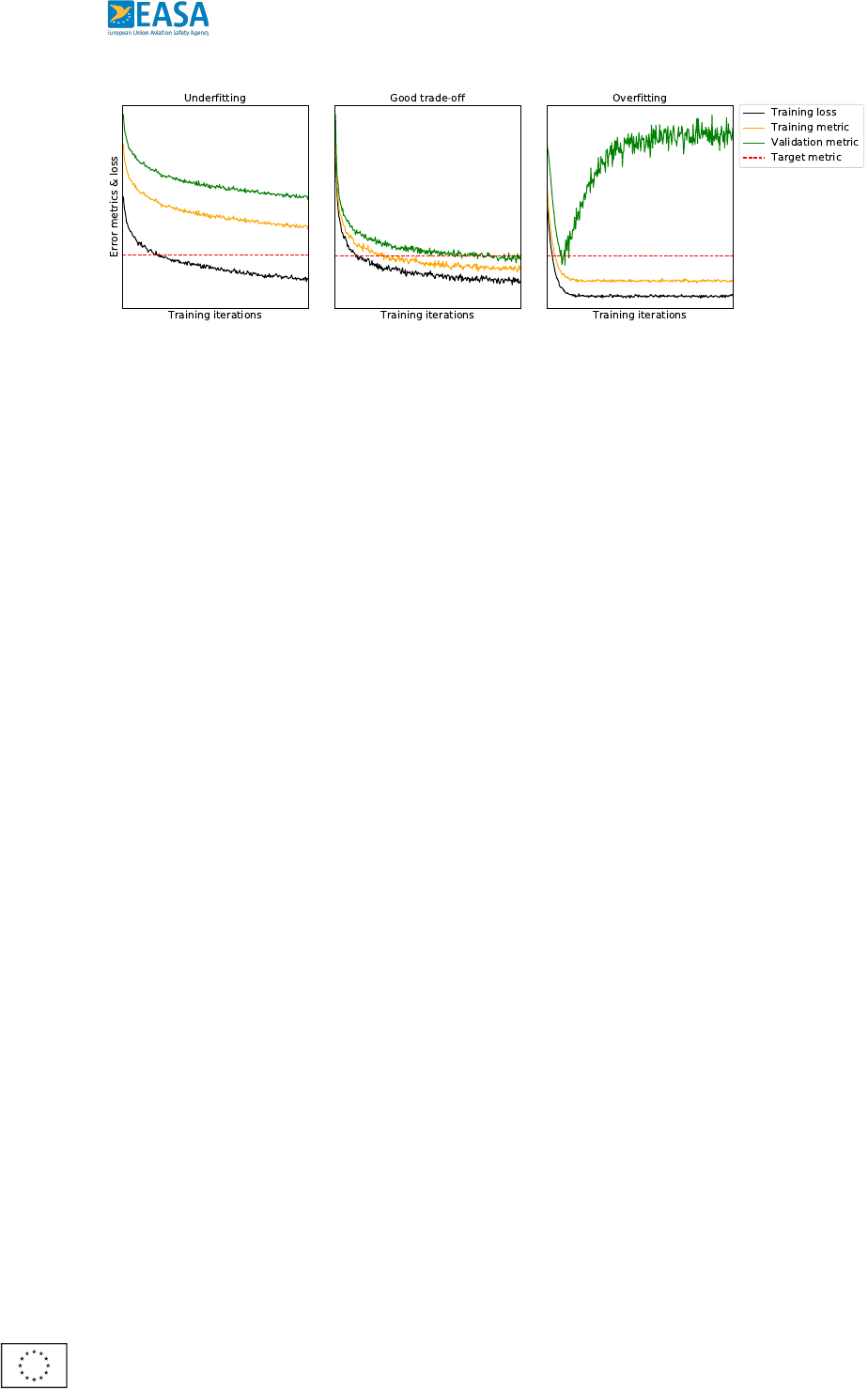
An agency of the
European Union
Daedalean – EASA CoDANN IPC Extract – Chapter 6 51
Figure 6.2: Three cases of approximation-generalization behaviors when training models. Early
stages of model training are typically underfitting (left), as the m odel parameters have not
fully approximated the target function yet. Overfitting behavior (right) can be observed when
the model parameters have memorized the training data, resulting in the model’s inability to
generalize to unseen data. Good model parameters (center) both approximate the training
data well and generalize to unseen data at the same time. Note that each of the three cases
visualizes a single error metric computed on the training and validation datasets (where lower
is better), but there might be several error metrics.
6.3 Training phase verification
6.3.1 Training curves
Early indications of adequate learning properties can be obtained by examining the approximation-
generalization behavior (see
Section 5.3.2) of the model as training progresses. This behavior
is captured by gathering losses and metrics during the training phase and plotting them into
so-called training curves.
Most notably, the relationship between the training loss, the training error metrics, and the val-
idation error metrics are indicative signs of whether the model parameters are in an underfitted
state, an overfitted state, or a “satisfactory” state. This satisfactory state is often referred
to as a state where the model has converged into an optimal trade-off between approximation
and generalization.
Examples of training curves and how they relate to various levels of over-/underfitting and
training process stages can be found in
Figure 6.2. These training curves should be provided
as part of the design phase artifacts to validate that trained model has converged correctly.
6.3.2 Reprod ucibility and replicability
Reproducibility and replicability are key elements of the scientific method and so are they
for certification of machine learning-based systems, since learning assurances are based on
experiments and measurements.
In particular, any learning process that is run with the same inputs (training dataset D
train
,
learning parameters) should produce equivalent or similar models, despite parts of the learning
process being random (weight initialization, sampling, stochastic optimization, . . . ).
Model equivalence will be defined in Section 6.4.1: the model outputs are the same for every
input, up to some tolerance factor. From there, performance assurances of one model would
follow from performance assurances of the other.
There are further ways to measure model similarity, such as:

An agency of the
European Union
Daedalean – EASA CoDANN IPC Extract – Chapter 6 52
• Distances between the parameters/weights (from which model equivalence could follow);
• Correlation of network activations (on intermediary and final layers), using various corre-
lations measures (see the survey and new methods given in [
Kor+19]).
These are distinct notions from model equivalence and the similarity measure to use should be
determined and analyzed as part of the Safety Assessment.
6.3.3 Multiple version dissimilarity considerations
From [ED-12C/DO-178C, Section 2.4.2]:
“Multiple-version dissimilar software is a system design technique that involves
producing two or more components of s oftware that provide the same function in
a way that may avoid some sources of common errors between the components.”
It is also possible to take advantage of multiple version dissimilarity for machine learning sys-
tems, in a strategy called ensemble learning [
ESL, Chapter 16].
In ensemble learning, multiple models are combined to perform the same function. Typically,
through the “wisdom of the crowd effect”, the final predictions will be more accurate and/or
with less variance. This can be easily seen through the following two examples:
1. Given 21 classifiers each having independent error rate ε = 30.0%, one forms a classifier
by taking the majority vote. The error rate of the new classifier is only
20
X
i=12
20
i
ε
i
(1 − ε)
20−i
< 0.52%;
2. If X
1
, . . . , X
n
are independent variables with mean µ and variance σ
2
, then the average
X =
1
n
P
n
i=1
X
i
still has mean µ, but has lower variance σ
2
/n .
Models in an ensemble can differ in multiple ways, for example:
• The model parameters are initialized differently at the beginning of training, as proposed
by Lakshminarayanan et al. [
LPB17];
• They are trained with different learning algorithms;
• They could be shown a different subset of data (but evaluated on the same test set).
There exist several methods for combining models, see [Zho12]. For example:
• Given a learning algorithm, Bootstrap aggregating (bagging) proposes to train a certain
number of models using random subsets of the training dataset and then average (or
take majority voting for classification) the predictions. The goal is to reduce variance,
as in the second example above. See also e.g. [
ESL, Section 8.7];
• Boosting algorithms work by successively training models, where previously misclassified
example are given higher weights for the training of the s ubsequent models. The models
are then combined with a weighted average or majority vote. The goal is to reduce bias
and eventually variance. For example, random forests combine simple decision trees with
boosting (see e.g. [
ESL, Chapter 10]).
Usually, a requirement of ensemble learning is that the errors of each model are independent (as
seen in the examples above). This could be probed using statistical testing and the performance
gains can be mathematically estimated. An example will be given in
Chapter 9.

An agency of the
European Union
Daedalean – EASA CoDANN IPC Extract – Chapter 6 53
Measuring ensemble agreement An ensemble allows to measure the agreement score of the
individual classifiers during the design phase.
Section 6.6.4 explains how this can be used for
runtime/uncertainty monitoring during the operational phase.
6.4 Machine learning model verification
The ability to verify model behavior during the design phase helps establish trust in the model’s
performance during operation. This section explores several verification strategies, from run-
ning systematic tests to formally proving model properties, and discusses their limitations and
applicability in the context of safety-critical applications.
6.4.1 D efinitions
Algorithm robustness and model robustness
According to the definitions of Section 5.1,
the learning algorithm F during t he training phase produces a trained model
ˆ
f
(D
train
)
: X → Y ,
which represents a function mapping from the data input space X to prediction space Y . It
is often important to understand, which properties this function exhibits when it comes to
perturbations of input, i.e. how stable it is. This task is known as sensitivity analysis.
Phase Input Output Relevant fluctuations Type
design D
train
F(D
train
) Those in the train-
ing dataset (replace-
ment of data points,
additive noise, label er-
rors etc).
learning algo-
rithm stability
operational x ∈ X,
F(D
train
)
F(D
train
)(x) Those in the data in-
put and prediction out-
put or in the model it-
self (model alteration).
model stability
Table 6.1: Two sources of robustness: algorithm and model stability.
To this end, there are two sources of instability which might be considered here and they
naturally stem from the fact that there are two inputs contributing to the final prediction of
such a trained function: the training dataset and the datapoint which is fed to a trained model.
This is summarized in
Table 6.1.
The above two sources of fluctuations allow for slight variability in definitions of robustness.
Robustness of learning algorithms (
Figure 6.3, (a,b)) is the type of robustness which ensures
that the produced model does not change a lot under perturbations of the training dataset
D
train
. Traditionally, this is referred to as learning algorithm stability. Robustness of trained
models (
Figure 6.3 or model stability, (b,c)) refers, on the contrary, to keeping input-output
relations
2
of a trained model, e.g.:
kx
′
− x
′′
k < δ ⇒ k
ˆ
f (x
′
) −
ˆ
f (x
′′
)k < ε, where x
′
, x
′′
∈ X and δ, ε ∈ R
>0
.
2
Here and below the notion of “closeness” is deliberately not defined. It can be any norm or any distance in
any respective space, whose choice is specific to the task at hand. For example, in case of adversarial attacks,
the “closeness” is typically defined as per-pixel p-norm. In case of rotation invariance, the “closeness” is a more
complex notion, captured by norms such as the Wasserstein norm.

An agency of the
European Union
Daedalean – EASA CoDANN IPC Extract – Chapter 6 54
(a) Original classification (b) Training phase perturbation (c) Operational phase perturbation
Figure 6.3: A simple showcase illustrating the notions of learning stability and inference ro-
bustness. Margin-maximization classifier (in this case, linear SVM) is (a → b): not robust to
perturbations during training — one datapoint is removed leading to change in the resulting
model, but (b → c): is robust to perturbations during inference — all datapoints are now
perturbed and classification result yet remains the same.
6.4.2 O verview of neural network verification methods
There is a tendency (see Sun et al. [SKS19] and Liu et al. [Liu+19]) to divide all verification
methods into several (partially intersecting) categories:
• Coverage-based white-box testing: aims at running trained models through a systematic
testing of both the extrinsic (outputs) and intrinsic (architecture-dependent properties)
behaviors of the model;
• Falsification: adversarial attacks that make use of special artifacts of the training process
to generate corner-cases for the trained models;
• Formal verification: aims at obtaining formally-derived worst case robustness bounds.
(a) Input image (b) Intrinsics: activations (c) Analysis of statistics
Figure 6.4: White-box testing aims at analyzing the network extrinsics and intrinsics when
being run through a set of tests. Example of a final approach to a runway (see the ConOps,
Table 4.1). (a → b): Input image results in a set of inner activations “reacting” to runway
semantics (approach lights and touchdown) or geometry (lines) (b → c): the latter is analyzed
to check that the intrinsics behaves as expected, or to generate new test examples.

An agency of the
European Union
Daedalean – EASA CoDANN IPC Extract – Chapter 6 55
Soundness and completeness Verification algorithms can be sound and complete (those prop-
erties are not mutually exclusive). Informally speaking, one says that a verifier is sound, if the
fact that it returns “property holds” implies that the property actually holds. One says that a
verifier is complete, if the fact that the property actually holds will imply that such a verifier
returns “property holds”. Intuitively, a sound verifier minimizes false positive returns and a
complete verifier minimizes false negative returns (see
Figure 6.5).
property
actually
holds
verifier
confirms
property
soundness
completeness
Figure 6.5: Soundness ensures that if the verifier returns “property holds”, then it actually
holds. Vice versa, completeness ensures that if the property holds, the verifier will be able to
“catch” this.
Verification via white-box testing Methods of this group aim at efficient procedures to explore
the behavior of a neural network through testing. “White-box” in this context (see
Figure 6.4)
refers to the fact that the test is allowed to see not only the final output behavior (“extrinsics
tests”), but the behavior of the neural network’s internal parameters — such as neural cover-
age, activation patterns, etc. Typical examples of the methods are DeepXplore [
Pei+17] and
DeepTest [
Tia+18].
Verification via semi-formal falsification Methods of this group apply a white-box approach
in an attempt to generate “hard” test examples for the neural networks, hence “falsification”.
However, they do not provide any formal guarantees of the existence or non-existence of
an edge/failure case for the network, hence “semi-formal”. Such methods typically do not
guarantee completeness, but attempt to maximize soundness, i.e. expand test coverage in
meaningful and efficient ways. Recent examples include [
DDS19] and [Zha+18b], which use
specialized search procedures for finding hard test cases.
Verification via formal approaches This set of methods attempts to solve the main issue of
the verification approaches above: it is impossible to test the network outputs on the set X of
all possible inputs, due to the continuum cardinality of the latter. To circumvent this issue, it
is suggested to formally verify verification properties which are generally defined [
Liu+19] as
“if-then” statements of a predicate form:
prop
ˆ
f
(X
c
, Y
c
): x ∈ X
c
⇒ F(D
train
)(x) ∈ Y
c
,
for X
c
⊆ X, Y
c
⊆ Y . The pair C = (X
c
, Y
c
) is called verification constraint.
For a given verification constraint C, a typical formal verification algorithm shall output one of
the following types of verification results (see Liu et al. [
Liu+19]):
• Counterexample result: the verification algorithm finds an input x
∗
∈ X
c
that violates
the constraint:
ˆ
f (x
∗
) 6∈ Y
c
(
Figure 6.6b). In plain language, it answers the question:
“Are there any inputs that violate the given constraint?”.
Methods that can be mentioned here include Reluplex [Kat+17] or ReluVal [Wan+18];
• Adversarial result: for any given input x
0
∈ X
c
, the verification algorithm finds perturba-
tion guarantees, that is, the largest possible ε-ball around x
0
, such that the constraint is
satisfied:
min ε such that
ˆ
f (B
ε
(x
0
)) 6⊆ Y
c
,
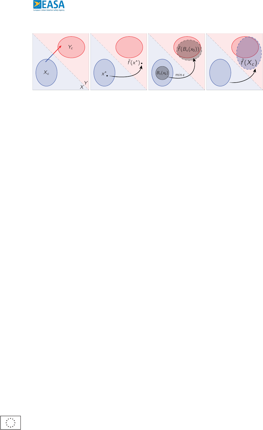
An agency of the
European Union
Daedalean – EASA CoDANN IPC Extract – Chapter 6 56
constraint
(a) Legend (b) Counterexample result (c) Adversarial result (d) Reachability result
Figure 6.6: Three types of formal verification results. (a): notation. Light-blue and light-
red areas X, Y depict input and output spaces; blobs X
c
, Y
c
depict the constraint sets. (b):
a counterexample result represents a single datapoint x
∗
that violates the constraint. (c):
an adversarial result represents the minimum perturbation ε of the input around x
0
that still
violates the constraint. (d): reachability result represents the image
ˆ
f (X
c
) in the output space.
effectively ensuring that if the constraint input set X
c
does not exceed this perturbation,
the whole constraint is s atisfied (
Figure 6.6c). In plain language, it answers the question:
“What is the largest tolerable perturbation to the input constraint such that the output
constraint is still satisfied?”
Formal verification methods that return adversarial results include for example DLV [
Hua+17]
which aims at searching adversarial guarantees along with falsifying the properties;
• Reachability result: for the constraint X
c
, the reachability result outputs its image
ˆ
f (X
c
) (
Figure 6.6d). In plain language, it answers the question: “What are the out-
puts for the given set of inputs?”
Methods of this group include maximum sensitivity approach [
XTJ18] (called MaxSens
in [
Liu+19]), exact reachability analysis of [XTJ18] or DeepZ, a method of [Sin+18].
The latter method uses a framework of abstract interpretation [
CC77] which aims at
constructing tight over-approximation bounds for each of the transformations in the
neural network.
6.4.3 Challenges and issues of formal verification methods
Verification of machine learning models and, more precisely, deep learning models has gained
significant attention from the research and industrial community, primarily as a means to
mitigate the risks typically exhibited by such models (learning instability, model instability,
inequivalence, etc.). This has led to extensive work in various specific sub-domains. Despite
this ongoing extensive effort, several challenges yet persist, as outlined by Leofante et al.
[
Leo+18]:
Computational costs and scalability Verifying NNs is a computationally hard problem (falling
into the category of NP -complete ones, see [
Kat+17]). The approaches outlined above gen-
erally struggle to scale well both in the number of hidden units and the number of hidden
layers. An intuitive reason for that is the fact that the amount of constraints for the underly-
ing optimization problems (primal, dual, SAT, SMT) grows exponentially with the number of
layers.
Guarantees There is an inherent trade-off between the runtime of a verification algorithm and
the completeness of results it returns. A possible intuitive explanation would refer to the fact

An agency of the
European Union
Daedalean – EASA CoDANN IPC Extract – Chapter 6 57
that many methods (especially those returning reachability results) make use of various over-
approximations for network operations (e.g. ReLU activations). Such approximations trade
exactness with computational simplicity.
Applicability The applicability of formal verification methods depends on:
• The type of network activations. Verification methods are generally not universal, i.e.
most of them target specific activations such as ReLU or piecewise linear. There are
only a few methods that extend to arbitrary types of activations and typically come at a
cost of runtime, completeness or over-approximation;
• The type of network architecture. Very few methods aim at verifying recurrent neural
networks (RNNs). An advantage of the feed-forward architecture is that the algorithm
does not need to unroll complicated looping execution branches. Recent work that
investigates RNNs is [Aki+19].
Lack of benchmarking Since there are many desirable properties that may be required from
typical verifiers (speed, completeness, soundness), it would be natural to benchmark them on
some common tasks, similar to how modern machine learning models are benchmarked on
common datasets.
Comparison with software formal verification It is worth noting that a software engineering
counterpart to model verification is provided in [
ED-216/DO-333]. However, given the com-
plexity of the input space and the number of parameters for a modern deep neural network
(on the order of millions), it is infeasible to exhaustively or nearly-exhaustively verify all possi-
ble computation branches and build exact reachable sets of outputs. This is the reason why
there exist a lot of sub-divisions in neural network verification methods, ranging from exact to
approximate.
6.4.4 Conclusion
Machine learning model verification represents a rich class of methods which can provide rig-
orous performance guarantees that are highly desirable for safety-critical applications, e.g. to
mitigate unexpected behavior. These methods establish robustness properties of neural net-
works, such as stability under random or adversarial perturbations, or full coverage of poss ible
outputs.
More recent verification methods, including semi-formal approximate methods, provide a promis-
ing path to overcome the computational challenges described in this chapter. The applicability
of new approaches coming from this field should be constantly evaluated.
6.5 Inference stage verification
The inference model verification consist of identifying the differences introduced by the im-
plementation phase and verifying the conservation of the training model properties after the
transformation to the inference model.
This report does not focus on these verification steps, which will be addressed in future work.
6.6 Runtime monitoring
[ED-12C/DO-178C, Section 2.4.3] describes safety monitoring as a means to protect “against
specific failure conditions by directly monitoring a function for failures that would result in a

An agency of the
European Union
Daedalean – EASA CoDANN IPC Extract – Chapter 6 58
failure condition”. This section investigates how such monitoring should be done for machine
learning models during the operational phase.
Correct operational space As seen in the previous chapter, most of the arguments guaran-
teeing correct output rely on the assumption that the input data follows the target distribution
X against which the model has been trained. Therefore, a first concern is to verify that this
hypothesis holds during operation.
Quantification of uncertainty Furthermore, in line with the system architecture (Section 4.2.1),
it is assumed that machine learning models receive raw sensory input, perform low-level fea-
ture extraction and classification. Their outputs are then fed into higher-level systems, such
as tracking algorithms or decision making systems. In this setting, models must not only be
accurate, but one would also like to obtain a measure of their uncertainty. If the network
were to output an accurate uncertainty alongside its predictions, results with high uncertainty
could be discarded by higher-level systems. Understanding a model’s uncertainty can avoid that
higher-level systems blindly rely on incorrect results. For example, in assistive systems, a good
fallback option would be to pass control back to a human.
6.6.1 Traditional software considerations
While [ED-12C/DO-178C] m entions that monitoring functions can be implemented in hard-
ware, software, or a combination of both, the following focuses on software only.
Separation of concerns A common approach is to separate separate functionality execution
from monitoring. For example, Koopman, Kane and Black [
KKB19] refer to this as the “Doer ”
and “Checker” separation. The Doer subsystem executes the normal, untrusted functionality
(e.g., execution of a neural network) while the Checker subsystem implements failsafe behavior.
That way, if the Checker knows how the behavior of the Doer looks like in normal conditions, it
can flag any abnormal output which can be taken into account by higher-level decision making
systems.
This can and should of course be applied to the operation of machine learning models.
6.6.2 What can be encountered during operat ion?
Ideally, the distribution of the input provided to machine learning models during operation
should precisely match that of the input space X identified during the design phase. This can
however not be fully guaranteed in practice and, unfortunately, it is as easy to come up with
aphorisms about expecting the unexpected as it is hard to define it in practice. Nonetheless,
it is important to at least obtain a broad categorization of any input that could be practically
observed during operation, so that risks associated with out-of-distribution scenarios can be
properly mitigated. Below, such a classification is attempted:
Expected input These are samples coming from the distribution X , say having high enough
probability.
Long-tail examples / edge cases These are samples coming from the distribution X , but
that have low or very low probability. This implies that the model might not perform well on
these inputs, even though the model metrics are high (since these are often taken as averages
over datasets).
Static Aberrations These are sensor artifacts that perturb samples from X , such as (in the
case of a camera) humidity condensation, unexpected aircraft parts in view, camera misplace-
ments, bent parts, etc. They can be, but are not exclusively malicious in nature.

An agency of the
European Union
Daedalean – EASA CoDANN IPC Extract – Chapter 6 59
Dynamic Aberrations These are dynamic sensor artifacts that perturb samples from X such
as (in the case of a camera) laser pointing, physically blocking camera view, image capture
processing noise, etc. They can be, but are not exclusively malicious in nature. This input
category relates to the data accuracy errors described in
Section 6.2.3.
Adversarial attacks These are methods to purposely produce input (in the target distribution
X or not) on which the model
ˆ
f gives “bad” approximation to f (say with respect to one of
the metrics m).
• White-box adversarial attacks require access to the model intrinsics (architecture, weights,
training data, . . . );
• Black-box adversarial attacks are model-agnostic: one assumes that the adversary only
has access to the output of the model.
Others The final category comprises other types of out-of-distribution samples, such as (in
the context of the ConOps from
Chapter 4) images of a geographic region not contained in
X , or images t aken after 9pm.
6.6.3 D etecting out-of-distribution data
Out-of-distribution/anomaly/novelty/outlier detection was already touched on in Section 6.2.8
and the generic distribution discriminator D : ⊔
n≥1
X
n
→ [0, 1] used to v erify the distribution of
the design phase datasets can directly be used to ensure that the inputs during the operational
phase match the design distribution X . For example, one can set thresholds 0 < δ
1
< δ
2
< 1,
such that a sample x ∈ X satisfying
• D(x) > δ
2
is considered in-distribution;
• D(x) ∈ [δ
1
, δ
2
] is considered an edge case;
• D(x) < δ
1
is considered out-of-distribution.
Note that more generally, discriminators can be agnostic to the model
ˆ
f that they might be
used with, or actually use parts of it.
Section 6.2.8 referenced two surveys on outlier detection methods. Another recent example,
this time using the intrinsics of the model, is the Out-of-DIstribution detector for Neural
networks (ODIN) method by Liang et al. [LLS18].
6.6.4 Estimating uncertainty during operation
Uncertainty types
Understanding which different types of uncertainty a machine learning
model has, can help understand and mitigate operational risks. Der Kiureghian and Ditlevsen
[
DD09] identified seven high level sources of uncertainty, which they categorize into two types
of uncertainty:
1. Epistemic uncertainty refers to the situation where the model
ˆ
f has not been exposed
to the relevant input domain area X . In other words, the function’s parameters θ do not
correctly fit the input data.
2. Aleatory uncertainty refers to the intrinsic randomness in the data, which was introduced
in
Section 5.2.2. This can come from data collection errors, sensor noise, or noisy labels.
In other words, the model has seen such data during training but expects it to be difficult.

An agency of the
European Union
Daedalean – EASA CoDANN IPC Extract – Chapter 6 60
Crucially, the main difference is that epistemic uncertainty can be reduced by adding more data
to the training set, while aleatory uncertainty will always be present to a certain extent. Given
that there is complete dataset with a correct learning process as defined in
Sections 6.2 and 6.3
respectively, one can consider that all epistemic uncertainty has been sufficiently minimized
within the ConOps input domain.
Probability outputs and miscalibration of models Many machine learning models already
output a probability as their prediction (often the output of a logistic function, the result of
mapping any real number to [0, 1]). An example of this is the model described in
Section 4.2.1
(runway presence likelihood).
However, it has been shown that these probabilities are usually not calibrated, in the sense that
they measure likelihood, but do not match with the empirical error rates that would be observed
on data. For example, Guo et al. [
Guo+17] showed that modern neural network architectures
tend to suffer from overconfident probability estimates. Furthermore, Hendrycks and Gimpel
[
HG17] used this approach as a baseline to empirically demonstrate that model predictions are
not directly useful as confidence estimate to distinguish in- from out-of-distribution samples.
Still, there are m ethods to address this issue, such as simply rescaling the probabilities a
posteriori (a variant of Platt scaling), as suggested by [
Guo+17].
Other methods for measuring uncertainty There also exist multiple methods to estimate
the uncertainty of arbitrary models, that do not already intrinsically estimate it:
•
Section 6.3.3 explained that instead of training a single model, one can train an ensemble
of models. When used in operation, one expect the members of the ensemble to mostly
agree on their outputs (i.e. have low v ariance). On the other hand, “disagreement” can
be used to measure uncertainty.
• Variational dropout [
KSW15], or Monte Carlo dropout, is a Bayesian view on dropout
which applies dropout during both training and testing. It follows that if dropout is
applied during test time repeatedly, a probability distribution is obtained instead of a
point estimate. That probability distribution can then be used to obtain statistics such
as mean value and variance. For samples that the model has seen during training, one
intuitively expect a low variance around the mean. However, for unseen samples, a high
variance is expected among the forward passes. More generally, this implies that one can
estimate how well the model fits the mean and variance and use that as a measure of
confidence.
6.6.5 Risks and mitigation
Monitoring the operational input- and output space during operation by functionality separation
(
Section 6.6.1) is subject to the following non-exhaustive set of possible risks that one needs
to be mindful of. Sculley et al. [
Scu+14] have identified several risks that are relevant to
the runtime monitoring of machine learning models in operation and are referred to where
applicable. Aside risks specific to runtime monitoring, Sculley et al. identify other machine
learning related risks, but these are considered to be mitigated by [
ED-79A/ARP4754A] and
[
ARP4761] standards and the strict specification of ConOps in Chapter 4.
Assumption turns into fallacy First and foremost, it is important to realize that any means
to introduce robustness to undefined phenomena comes with inescapable assumption-making.
It is equally important to treat these assumptions as such at each stage during development
and testing. [
ED-79A/ARP4754A] and [ARP4761] define assumptions as “Statements, prin-
ciples and/or premises offered without proof” and provide guidelines and methods on how to
assess the assumptions made as a part of Functional Hazard Assessments. Consequently, every

An agency of the
European Union
Daedalean – EASA CoDANN IPC Extract – Chapter 6 61
assumption made on t he unknown space described by the designer should be held to iterative
scrutiny at each evaluation stage, which is described in more detail in
Chapter 9. For illus-
trative reference, assumption validation and adjustment is one of the first steps — the “first
iterations” — in the Fault Tree Analysis example given by [ARP4761, Appendix D.3.b].
Edge case or out-of-distribution? There is a fine line between edge cases (in-distribution
elements that are unlikely) and out-of-distribution samples. Given Operational Concept 1 from
Table 4.1, one can try to decide whether the following illustrative scenarios are edge cases or
out-of-distribution examples:
1. The input images are taken from an altitude of 1800M AGL, instead of the specified
800M AGL;
2. A solar eclipse darkens the camera view;
3. An airshow is being held next to the runway, resulting in an abnormal amount of visual
obstructions and distractions around the runway;
4. An unusual springtime flower “super bloom” happens around the runway.
The above examples highlight the difficulty of deciding whether a particular scenario is out-of-
distribution or an edge case. The classification can be subjective to the reader without careful
analysis. As an example, the first scenario is only clearly out-of-distribution after reviewing the
altitude parameters specified in the ConOps from this report.
Empirical out-of-distribution thresholds do not hold during operation Most methods that
estimate the distribution origins of inputs are thresholded methods, whether that is a threshold
on uncertainty, entropy, or other measures.
These thresholds are typically estimated during test phases and validated using more annotated
data. Specifically, human bias in selecting in- and out-of-distribution samples may be skewed
towards certain unknown distributions. For example, the list of scenarios in the previous risk is
a display of the author’s bias; an unbiased observer, i.e. somebody that has not seen that list,
may think of entirely different cases.
The discriminating threshold that was found during the test phase may not hold during oper-
ation, resulting in unjustified amounts of in-distribution samples labeled as out-of-distribution
(a false positive; the threshold was placed too high), or out-of-distribution samples labeled as
in-distribution (a false negative; the threshold was placed too low).
Scully et al. [Scu+14] address this risk in section “Fixed Thresholds in Dynamic Systems”,
under the scenario that these thresholds are tuned manually. The authors propose to mitigate
this strategy by tuning these thresholds on held-out data, which is exactly the method outlined
above. Rather, an emphasis should be placed on validating this held-out dataset and its
representativity of the target ConOps, as described in
Section 6.2.
Common mode failures in ensembles This final risk of common mode failure applies to using
multiple versions of the same model architecture for joint decision making as described in
Section 6.3.3. A common mode failure describes the event of multiple instances failing in the
same manner, where they were otherwise considered independent and therefore should not fail
in such a way.
It specifically addresses the risk of assuming that having more versions of slightly different, but
still the same component increases independence, when they actually have a common unseen
flaw and/or vulnerability. Similar to the first risk (that addresses assumptions specifically),
these assumption should be thoroughly tested through safety assessments.
Section 9.4 is
dedicated to the description of the way in which such assessments should be conducted to
prevent common mode failure.

An agency of the
European Union
Daedalean – EASA CoDANN IPC Extract – Chapter 6 62
Sculley et al. [
Scu+14] address a similar risk in “Monitoring and Testing”, under the scenario of
a single operational model. The authors propose two starting points for mitigation strategies.
The first mitigation approach is using the prediction bias as a diagnostic for indicating sudden
changes in the environment. The second mitigation proposal suggests to enforce a limit on
the system’s actions as a sanity check.
6.7 Learning Assurance artifacts
The following list provides a summary of the minimum (i.e. not exhaustive) artifacts whose
generation is recommended during the development of airworthy machine learning models:
PLAC: Plan for Learning Aspects of Certification A summary of all aspects of machine
learning safety and how it relates to certification.
The training, validation, and test datasets D
train
, D
val
, D
test
⊂ X. alongside evidence that
the datasets satisfy the data quality requirements outlined in
Section 6.2.
The design phase details. Model architecture (including the type of NN, number of lay-
ers/neurons, activation function(s), loss function), training procedure and hyperparameters
(including random seeds), training curves (see
Section 6.3).
The end model
ˆ
f : X → Y .
The input distribution discriminator D : ⊔
n≥1
X
n
→ [0, 1]. To ensure that the datasets
considered are independently sampled from the input space X , see
Section 6.2.8. This dis-
criminator should satisfy the conditions therein with respect to the training, validation, test,
and out-of-distribution datasets.
An out-of-distribution dataset D
ood
. To test the distribution discriminator.
The error metrics m used to evaluate the model, and corresponding performance thresh-
olds.
These should be determined prior to the training process and included here.

An agency of the
European Union
Chapter 7
Advanced concepts for Learning As-
surance
In the last chapter, elements of Learning Assurance that can be considered absolutely necessary
for the operation of complex machine learning algorithms in any safety-critical application are
provided. This chapter gives a discussion of more advanced concepts alongside their potential
risks and benefits. Some of the concepts presented here are active areas of research and the
reader is invited to follow progress in these closely.
7.1 Transfer learning
In real-world applications, data collection and model training is often expensive, and models for
related tasks and domains should be able to share characteristics. In short, the idea of transfer
learning is to use information from one model to help obtain another one on related tasks
and/or domains, in a less data- and/or computation-intensive way. Parallels can be drawn with
human behavior: it is easier to learn how to drive a truck, if one already knows how to drive a
car.
There exis t multiple variants of transfer learning: transfer between tasks, between input types,
between input domains, etc. For simplicity, this section will focus on the important category
of homogeneous domain transfer (albeit a majority of the remarks apply to other variants).
Namely,
• one has a model
ˆ
f : X → Y that has performance guarantees when the inputs x ∈ X
follow a probability distribution P (i.e. X = (X , P )), and
• one would like to obtain a model
ˆ
f
T
: X → Y that performs well when the inputs x ∈ X
are sampled from a probability distribution P
T
(i.e. the new domain is X
T
?(X, P
T
)).
In other words, the type of outputs and the task remain the same, but the underlying probability
distributions change. A simple but important example is when X is a set of RGB images
collected over a specific geographical region and one would like to make the model work in a
different region (with different visual characteristics).
7.1.1 D omain transfer methods
There are many methods to perform transfer learning, up to the extent that giving a complete
overview would deserve a report of its own. Instead, the reader is referred to [
PY09; WD18]
63

An agency of the
European Union
Daedalean – EASA CoDANN IPC Extract – Chapter 7 64
Training
Model 1 Model 2
Accuracy Precision Accuracy Precision
Real data (baseline) .719 .792 .781 .792
Synthetic data
.643 .753 .637 .755
Synthetic data, fine-tuning on real data
.767 .809 .787 .800
Table 7.1: Training on synthetic data, table from [Gai+16]. Higher scores are better.
and the following rather explains a few selected methods to motivate the discussion on risks in
the next section.
Based on the availability of labels, the methods can be classified into supervised (requires
labels), semi-unsupervised (partially requires labels) and unsupervised (does not require labels).
If the domain gap is small enough, unsupervised methods would be a prime choice, as they
require no additional annotated data, only data from the new domain. In any case, these
methods usually have trade-offs between the amount of data (annotated or not) necessary,
and the complexity added on top of the original learning algorithm.
Note that the results presented below are mostly empirical. While general patterns can be
observed, no general statement can be made, and performance gains must be assessed on a
case-by-case basis, in the setting of
Chapters 5 and 6. In other words, it is the final model that
has to be evaluated, and no credit can be directly taken from the performance of the original
model on its original input space. This will be further explained in Section 7.1.2.
Fine-tuning To perform homogeneous domain transfer, one might simply resume the learning
algorithm F used to obtain the original model at the end of the training phase, and continue
training with data from X
T
instead of the data from X used so far. Note that fine-tuning is a
supervised approach.
At the beginning, the loss will be higher than the one seen at the end of the first training phase,
but the additional training steps should help bring the loss closer to the earlier one.
A few examples of this approach are the following:
• Girshick et al. [Gir+14] have demonstrated that supervised, domain-specific fine-tuning
is an effective method to learn high capacity models even when the target domain data is
scarce. Using a model that was trained on the large ILSVRC dataset, the authors observe
an 8% increase in the mean average precision metric when fine-tuning using the smaller
PASCAL dataset compared to a m odel trained on the PASCAL dataset from scratch.
• Gaidon et al. [
Gai+16] observe the scores in Table 7.1 on a multi-object tracking model,
evaluated on real data. Note that for evaluation on real data, synthetic-only training is
always worse than real-only training, which is also always improved by synthetic training
followed by fine-tuning on real data.
• Raghu and Zhang et al. [
Rag+19] provide insights into the effect of transfer learning be-
tween a benchmark natural image domain [
ImageNet] and two medical image domains.
Among other findings, the authors most notably demonstrate that transfer learning does
not always significantly improve model performance, and that smaller model architec-
tures trained solely on the target domain can perform comparably to larger, fine-tuned
architectures. This underpins t he point made earlier that performance gains must be
measured on case-by-case bases.

An agency of the
European Union
Daedalean – EASA CoDANN IPC Extract – Chapter 7 65
Bridging the domain gap as a pre-processing step Another approach is to try to make input
from the new domain “look similar” (i.e. have the same distribution) to the original inputs
as a pre-processing step. If X (resp. X
T
) is constituted of synthetic (resp. real) images,
this pre-processing might make “real images look synthetic”, for example by adding some blur
or sharpening edges. Of course, this pre-processing function can also be learned through as
complex machine learning model, trained on samples the two domains.
As an example of this approach, Zhang et al. [
Zha+18a] train (among other strategies) a model
on synthetic data, and evaluate it on real data as is, or after transforming it with a domain
adaptation function. The first naive method gives a mean intersection over union score of
29%, while the second one improves this to 46%.
More advanced approaches More complex methods for domain adaptations can for example:
• Adapt not only the domain, but the representations/features inherent to the original
domain;
• Perform the adaptation while jointly optimizing for the performance of the task at hand
(this could be semi-supervised or supervised).
For such examples, the reader is referred to [GL15; Zha+18a; Shr+17; SS14] (as well as the
survey [
WD18]. In there, Ganin and Lempitsky [GL15] propose an approach where the final
predictions are based on input representations t hat are discriminative and invariant to target
domain transfer. In digit image classification, the authors show performance increases ranging
from 42.6% − 79.7% when comparing their method to models that were only trained on the
source domain. The work of Zhang et al. [
Zha+18a] is an example of joint task optimization.
7.1.2 Risks and mitigation
Transfer learning can provide the advantage of reducing the cost of creating models (be it
in terms of data, computations, or other), but new risks are also added, compared with the
design pipeline handled in the previous sections. In this section, important risks are underlined
and suggestions to mitigate them are provided.
Performance verification As already noted in Section 7.1.1, it is fundamental that the per-
formance of the “transferred” models are evaluated on the target input space, rather than
taking any safety credit from the performance of the original model on the original input space.
Domain transfer is mainly an empirical method, whose results must be verified. The risk in not
doing so can be seen in the phenomenon exposed in the next paragraph.
Negative transfer When the source domain and target domain are sufficiently unrelated, it
gives rise to the risk of negative transfer. This is a phenomenon where the source domain X
contributes to poor performance of the target model
ˆ
f
T
. A prerequisite for transfer learning,
regardless of the availability of target domain labels, is the availability of a representative test set
for the target function. See also “Correct optimization target” below for a possible mitigation
stratgy.
Transfer from publicly available models A common form of transfer learning is through the
use models pre-trained on public datasets (see e.g. He et al. [
HGD19]; for neural networks,
this is also sometimes called “weights initialization”), which can be seen as domain and/or
task transfer. When used for safety-critical applications, one should consider:
1. It may be more difficult to verify that the correct Learning Ass urance requirements have
been fulfilled;

An agency of the
European Union
Daedalean – EASA CoDANN IPC Extract – Chapter 7 66
2. The “link to the intended function/absence of unintended function” is lost or harder to
keep track of;
3. The ability to train several models on different random weight initializations (see Sec-
tion 6.3.3
) is lost.
In other words, the full training process should be done in a way to follow the recommendations
exposed in this document.
Correct optimization target As mentioned in Chapter 6, the loss function (whose value is
minimized during the training process) should be a good proxy for the metrics of interest. In
transfer learning, the function optimized might however not be directly related to the metrics
(or a loss) of the target task anymore.
Ideally, the link between the transfer learning method and the optimization of the target metrics
should be shown.
Transfer algorithms Recall that transfer methods can be learning algorithms, as well as clas-
sical algorithms. In the first case, the transfer algorithm should as well satisfy the Learning
Assurance requirements outlined in this chapter. In the second case, the transfer algorithm
should follow usual software airworthiness requirements, e.g. [
ED-12C/DO-178C].
7.1.3 Retr aining and recertification
Transfer learning is a means to modify a model that complies with the concepts of Learning
Assurance from
Chapter 6. Potential risks and possible mitigation strategies were described in
the sections above. This leads to a discussion of requirements for (re-)certification of a newer
or retrained version of such a model. Such modifications can be grouped into:
1. model update, the model is retrained with new or additional data without further changes
to its original functionality;
2. model upgrade, the model is retrained such that its original functionality is (partly)
changed.
These types of changes and the possible implications for recertification will not be addressed
further in this report and left for future work. In the meantime, the reader is referred to
[ED-79A/ARP4754A, Chapter 6].
7.2 Synthesized data
Acquiring high-quality data satisfying the requirements of Section 5.1 can be very costly, while
it is crucial that machine learning algorithms are tested and trained on a very large amount of
data. Consequently, the design and testing of safety-critical machine learning models should
rely on simulated/synthesized data, for which new data can be acquired at a very low cost once
a system is setup. By synthesized data, it is meant any data that was computer-generated or
any data from the target sensors that underwent a processing step that is not included in the
target operational system.
7.2.1 Examples and classification of synthesized data
To better understand the possible benefits and risks of using synthesized data, it is useful to
first give a categorized list of examples, roughly in increasing order of complexity/syntheticity:

An agency of the
European Union
Daedalean – EASA CoDANN IPC Extract – Chapter 7 67
Figure 7.1: Various transformations of the runway image on the top left.
Figure 7.2: Augmentation of real data for the task of object detection: pictures of objects to
be detected are pasted against a background. Note that some additions appear realistic (the
aircraft), while some do not (the helipads).
Basic transformations of real data This type of synthesized data includes applying geometric
transformations (t ranslation, rotation, scaling, flipping, cropping, deformation, . . . ) or trans-
formations of image attributes (brightness, noise, hue, . . . ) to real data. See Figure 7.1. It is
widely used in machine learning and usually known as “data augmentation”: see for example
[SK19].
More advanced transformations of real data It is also possible to perform transformations
that go beyond applying basic transformations to the existing pixels. A common example is to
“paste” new objects into existing images, e.g. adding cars randomly on empty roads, or adding
images of aircraft against a background (see
Figure 7.2). The bounding boxes of the objects
added are by definition known, so that there is no need to do new manual annotations. This
was studied by Peng et al. [
Pen+15], among others.
Fully or mostly synthetic data Finally, one can also generate data that is fully or almost
entirely synthetic, for example a 3D urban scene as in
Figure 7.3 using textures and geometries
partially collected from the real world. Such examples can be found in [
Gai+16; Ric+16], along
with analyses of machine learning models trained on this data.

An agency of the
European Union
Daedalean – EASA CoDANN IPC Extract – Chapter 7 68
7.2.2 Risks and mitigation
Section 5.3.2 explained that having data independently sampled from the target input space X
is essential to obtain models that perform well during the operational phase and to estimate the
expected operational performance. Thus, the problem of domain shift/bias (see Section 5.3.2)
is a particular concern when using synthesized data in the training/validation sets D
train
, D
val
or in the test set D
test
.
Handa et al. [
Han+16] noted that fine-tuning a synthetic semantic segmentation dataset (with
added noise) on real (target) data leads to an improvement of 5% in the per-class accuracy,
compared to simply evaluating the model trained on synthetic data on real images. Further
examples were given in
Section 7.1, on transfer learning:
• Gaidon et al. [Gai+16], who observe drops of up to 15% when passing from synthetic
to real data (while combining both leads to better results than using real data only);
• Zhang et al. [
Zha+18a], who report that a model segmenting road scenes trained on
a photorealistic video game (GTA5 [
Ric+16], see Figure 7.3) only achieves 29% mean
intersection over union on similar real images from the Cityscapes dataset [
Cor+16]
(while an improved transfer strategy raises this number to 46%).
Similarly, even natural transformations of real data could end up changing the distribution of
the training data (which would therefore not match anymore the target distribution of X ).
Hence, the key requirement is that synthetic data should never be used without proper analysis
and mitigation of the domain biases , no matter how realistic it looks. The risks and m itigations
for transfer learning from
Section 7.1 apply to this situation.
It is useful to note that there is a dissension between the recent claims of companies producing
synthesized data for training (e.g. that one can train high-quality models using only their data),
and the observations made in academic research (such as the aforementioned works) which
question such claims.
(a) Real image (b) Synthetic image
Figure 7.3: An image from the GTA5 synthetic dataset [
Ric+16] and from the Cityscapes
[
Cor+16] real dataset.
Use of synthesized data for testing Testing machine learning systems using synthesized data
is extremely useful and important, as it helps to find edge cases that almost never happen in
the real world or that would be difficult or very costly to reproduce.
However, testing using synthesized data can only supplement testing using actual data from
the distribution X that is expected in the operational phase and not to replace it. Otherwise,
the learning assurances (such as the theoretical guarantees) would not apply.
Here, one can diverge from [
EAS19] and [UL-4600] (at least in the current version), that claim
respectively that

An agency of the
European Union
Daedalean – EASA CoDANN IPC Extract – Chapter 7 69
“Partial certification credits may still be granted while using a non-conformed test
article, provided that the item to be evaluated is simulated with an adequate level
of representativity.”
“In order to ensure that credit may be taken from the [simulator/test rig] tests,
the [simulator/test rig] must be adequately representative for aircraft systems and
flight dynamics. At the same time the limitations for using the [simulator/test
rig] must be established. This objective can be achieved by a combination of a
controlled development process of the [simulator/test rig], simulator configuration
management, system models behavior (crosschecked when necessary with partial
system bench or flight test results, analysis, desktop simulation) and engineer-
ing/operational judgment. Currently, there is no detailed guidance available on
the qualification of simulators or test rigs for use as a Means of Compliance for
certification. [. . . ] Relying upon simulation results in arguing safety is typically
a practical necessity. Simulation results can be used so long as their accuracy is
justified, simulation run coverage is justified, and an appropriate non-zero amount
of physical testing is used to validate simulation results.”
7.2.3 Conclusion
Many safety-critical applications require a significant amount of training and evaluation data to
obtain strong performance guarantees. Both transfer learning and synthesized data (eventually
used jointly) allow to palliate a lack of data in the target domain and/or task, by taking
advantage of existing or easy to generate data from different domains/tasks. Beyond that, the
use of synthesized data can help identify edge cases and s imulate scenarios that are difficult or
impossible to produce in the real world.
However, this comes with additional risks, highlighted in the sections above, that need to
be mitigated to obtain the same levels of performance garantees as those given by the pri-
mary learning assurance processes exposed in this chapter until
Section 7.1. For example, no
claim can be made on the real-world performance of models trained on synthesized data, as
photorealistic as it might be, without a careful analysis.

An agency of the
European Union
Chapter 8
Perf ormance assessment
In this chapter, the performance assessment of machine learning components, and systems
including these, is discussed. In particular, the choice of adequate error metrics is analyzed,
along with possible risks of performing the model and system evaluations.
8.1 Metrics
Chapter 5 introduced a machine learning model
ˆ
f : X → Y as the approximation of a function
f : X → Y , learned through samples (x, f (x) + δ
x
) ∈ D
train
. The quality of the approximation
is measured by error metrics m : Y → R
≥0
, requiring that
m
ˆ
f (x), f (x)
be small on all x ∈ X. (8.1)
The learning guarantees presented in Chapters 5 to 7 ensure that (8.1) holds during the
operational phase, on average and up to some small failure probability. Therefore, one should:
1. Discuss adequate choices of error metrics and potential pitfalls, which is the goal of this
section;
2. Understand how to control the failure probability and strengthen the “on average” state-
ment into the validity of (
8.1) for all expected inputs. This will be done in Chapter 9
(Safety Assessment).
8.1.1 Context
Section 4.2 outlined that the machine learning systems considered in this report are part of
larger (sub)systems, and do not perform “end-to-end” functions by themselves (for example,
from perception to actuation). This is the case for the model involved in the example of
Chapter 4 (ConOps), which is solely responsible for the perception component of the visual
landing guidance.
Therefore, it is important to realize that the choice of error metrics must be understood in the
scope of the whole subsystem and use case, and not in isolation. To illustrate this risk, one
can easily imagine two systems using the same m odel
ˆ
f , where good performance of
ˆ
f with
respect to m (in the sense of (
8.1)) translates to adequate performance for the first system
but not t he second. For example, assuming the model performs object detection, an error
metric might penalize false positives and false negatives differently:
70

An agency of the
European Union
Daedalean – EASA CoDANN IPC Extract – Chapter 8 71
• the first system aims at identifying runways, as in
Chapter 4. In this case, one might
want to avoid false positives above all, i.e. avoid that the system predicts the existence
of runways even when they are not present;
• the second syst em aims at identifying other aircraft to avoid collis ions. In this case, it is
better to have false positives than to risk a collision, i.e. avoid that the system misses
other aircraft even when they are present.
The error metrics must be chosen so that they ensure good performance for the whole s ys tem
(ultimately the whole aircraft) in the context of the application and must become an artifact
of the development process for certification.
8.1.2 D ifferent tasks and metrics
By definition, error m etrics depend not on the input space X of the model but on the output
space Y . In machine learning, one usually distinguishes between two main types of tasks:
Classification When Y is a finite/discrete set, a model
ˆ
f : X → Y has to assign to each input
x ∈ X a “category” or “class” y ∈ Y . Rather than predicting directly a class, these models
usually predict a soft score , or a probability distribution over Y , namely a likelihood for each
class. This allows for finer decision making and error measurements. An example is the runway
presence detection from Section 4.2.1.
Regression When Y is an infinite/a continuous set, such as an interval [a, b] ⊂ R, a model
ˆ
f
aims at estimating the continuous responses f ( x ) ∈ Y to the inputs x ∈ X that the function
f represents. Predicting bounding boxes in an image (e.g. Y = [0, 1]
4×2
, as in the runway
corner detection from
Section 4.2.1) is an example of a regression task. As discussed for
classification, the predicted values can be provided along with uncertainty measures.
A model can perform a combination of classification and regression, such as t he one described
in
Section 4.2.1. Keeping the slicing philosophy from Section 4.2 in m ind, the performances
with respect to the two task types are usually considered separately, before being combined.
The latter can be done by simply using several error metrics or by combining several error
metrics into one (e.g. through a weighted sum, see
Section 5.2.5).
There are usually many possible metrics for any classification or regression task, and these
should be carefully selected tak ing
Section 8.1.1 into consideration. Generally, all relevant
metric choices should be analyzed and the validity and precedence of the ones chosen justified.
In practice it is recommended to consider several metrics throughout the whole process and this
should be preferred over dismissing an important metric or because of computational overhead.
In the next sections, a (non-exhaustive) s election of common metrics is given for both types of
tasks. Recall also that
Section 5.2.5 gave a complete example for the runway detection case.
8.1.3 Examples of classification metrics
As explained in Section 8.1.2, it is best to phrase a classification task into d categories as
finding a model
ˆ
f : X → [0, 1]
d
,
such that the ith coordinate
ˆ
f
i
(x) gives the likelihood that x belongs to class i, enforcing
P
d
i=1
ˆ
f
i
(x) = 1. The model approximates the “ground truth” function f : X → [0, 1]
d
, where
f
i
(x) = 1 if and only if x belongs to class i. The predicted class for x ∈ X can be set as
ˆg(x) = arg max
1≤i≤d
ˆ
f
i
(x). (8.2)

An agency of the
European Union
Daedalean – EASA CoDANN IPC Extract – Chapter 8 72
True
positive
Runway
Runway
False
negative
No Runway
False
positive
No Runway
True
negative
Ground
truth
Prediction
Figure 8.1: A confusion matrix that summarizes binary classification outputs.
Binary classification Any classification task into d categories can be viewed as d separate
binary classification tasks (i.e. d = 2 and for each class 1 ≤ i ≤ d, whether a sample belongs
to class i or not). The binary classification task, as defined in Chapter 4, to decide if a runway
is visible in the image or not, is a suitable example for this section.
The output of a binary classification model can fall into four categories: true positives, false
positives, false negatives and true negatives. For example, true (resp. false) positives represent
the case where the classifier predicts that a runway is visible and the image does (resp. not)
contain it. False (resp. true) negatives represent the case where the classifier predicts that a
runway is not visible and the image does (resp. not) contain it.
Figure 8.1 summarizes these
outcomes as a confusion matrix.
Class imbalances Even in a binary classification setting (but also for multi-class classifica-
tion discussed later in this section), calculating average metrics has to be done carefully. In
particular, the underlying class distribution will likely influence the evaluation results. Class
imbalances can cause significant misinterpretations of m odel performance. For example, the
accuracy metric
2
X
i=1
I (f
i
(x) 6= (ˆg(x) = i)) ,
where I is the indicator function taking value 1 if its boolean argument is true, and 0 oth-
erwise, could be chosen. However, if most x ∈ X have class 1 (corresponding for example
to background), the model will have high performance with respect to class 1 while having
abysmal performance on all other classes. A complete evaluation of a classification model’s
performance always requires considering the distribution of classes and different error types.
False positives and false negatives For each of the outcomes 1 ≤ i ≤ d, true (false) positives
and true (false) negatives can be counted using the metrics
m
TP
(
ˆ
f
i
(x), f
i
(x)) = I (f
i
(x) = 1, ˆg(x) = i) ,
m
FP
(
ˆ
f
i
(x), f
i
(x)) = I (f
i
(x) = 0, ˆg(x) = i) ,
m
TN
(
ˆ
f
i
(x), f
i
(x)) = I (f
i
(x) = 0, ˆg(x) 6= i) and
m
FN
(
ˆ
f
i
(x), f
i
(x)) = I (f
i
(x) = 1, ˆg(x) 6= i) .

An agency of the
European Union
Daedalean – EASA CoDANN IPC Extract – Chapter 8 73
According to the definitions of
Chapter 5, the numbers of true (false) positives and true (false)
negatives in a dataset D are given by
|D| · E
in
(
ˆ
f
i
, D, m
ζ
) =
X
(x,f (x))∈D
m
ζ
(
ˆ
f
i
(x), f
i
(x)),
where ζ ∈ {TP, FP, TN, FN}.
Precision is the proportion of correct of positive predictions by the classifier:
Precision(
ˆ
f
i
, D) =
E
in
(
ˆ
f
i
, D, m
TP
)
E
in
(
ˆ
f
i
, D, m
TP
) + E
in
(
ˆ
f
i
, D, m
FP
)
(8.3)
=
# of true positives
# of true positives + # of false positives
.
Recall Conversely, recall measures how many of the positive samples were detected by the
classifier:
Recall(
ˆ
f
i
, D) =
E
in
(
ˆ
f
i
, D, m
TP
)
E
in
(
ˆ
f
i
, D, m
TP
) + E
in
(
ˆ
f
i
, D, m
FN
)
(8.4)
=
# of true positives
# of true positives + # of false negatives
Note that the definition of recall is similar to that of precision but takes into account false
negatives instead of false positives. In the runway example above, this measures how many of
the runways were detected by the classifier.
F
1
score If necessary, precision (8.3) and recall (8.4) can be combined into a single score. The
F
1
measure considers both and is defined as
F
1,
(
ˆ
f
i
, D) =
2 · Precision(
ˆ
f
i
, D) · Recall(
ˆ
f
i
, D)
Precision(
ˆ
f
i
, D) + Recall(
ˆ
f
i
, D)
(8.5)
A classifier with high precision and recall has a high F
1
score.
A more general form of the F
1
score is the F
β
measure where β ∈ R
+
:
F
β
(
ˆ
f
i
, D) =
(1 + β
2
) · Precision(
ˆ
f
i
, D) · Recall(
ˆ
f
i
, D)
β
2
· Precision(
ˆ
f
i
, D) + Recall(
ˆ
f
i
, D)
(8.6)
While the F
1
score is the harmonic mean, F
β
allows a different weighting of precision and
recall. For example, F
2
weights recall higher than precision and F
0.5
places more emphasis on
precision than on recall.
Decision thresholds In (8.2), the predicted class i was the one with the m aximal soft score
ˆ
f
i
(x). In the binary case d = 2, this is equivalent to setting a decision threshold at t = 0.5,
namely
ˆg(x) =
(
1 if
ˆ
f
1
(x) ≥ 0.5
2 if
ˆ
f
1
(x) < 0.5,
Other thresholds t ∈ (0, 1) may be used, leading to the decision functions
ˆg
t
(x) =
(
1 if
ˆ
f
1
(x) ≥ t
2 if
ˆ
f
1
(x) < t,
ˆg = ˆg
1/2
and having different rates of false negatives/positives (and therefore precision/recall).
During operation, this threshold can also be used as a rejection threshold and prevent the
classifier from outputting a class at all. This is discussed further in
Section 6.6.

An agency of the
European Union
Daedalean – EASA CoDANN IPC Extract – Chapter 8 74
Figure 8.2: Precision-recall curve for binary classifier
Precision/recall curve The influence of the threshold t
i
on the precision and recall values can
be illustrated in a precision-recall curve as shown in
Figure 8.2. As t
i
is varied, different values
for precision and recall are obtained. A higher t
i
generally results in higher precision and lower
recall (or lower false positive and higher false negative counts). As t
i
is lowered, one expects
lower precision and higher recall (or higher false positive and lower false negative counts). This
is often referred to as the precision-recall trade-off.
For example, one would typically choose a high t
i
to ensure that the model only predicts that
particular class (e.g. predicts that the runway is present) if it is “very confident”. Conversely,
a lower t
i
would ensure that the model predicts a class even if it is “less confident”, i.e. less
runways are missed.
The favorable classifiers are those that maintain a high precision as recall increases. Such
classifiers have a high area under the curve.
Costs A downside of the aggregated F
1
score (and in fact many other aggregating metrics)
is that it gives equal importance to precision and recall. As illustrated in
Section 8.1.1, in
practice, different types of error types have different associated costs with it. One may want
to penalize certain erroneous outcomes more than others. This is why it is recommended to
always report precision and recall separately.
Multiclass classification False positive and false negatives among all classes can be counted
by considering the error metrics
m (
ˆ
f (x), f (x)) =
d
X
i=1
I (f
i
(x) = 0, ˆg(x) = i) , resp.
m (
ˆ
f (x), f (x)) =
d
X
i=1
I (f
i
(x) = 1, ˆg(x) 6= i) .
Micro vs. macro averages The above considered any classification task into d categories
as d binary classification tasks and the performance was evaluated separately for each class.
Calculating an aggregated score over all classes could, for example, be helpful to compare
several models against each other. For this, two approaches can be considered:

An agency of the
European Union
Daedalean – EASA CoDANN IPC Extract – Chapter 8 75
Figure 8.3: Computation of the intersection over union (IoU) of two masks and examples. The
Jaccard distance is respectively 1, 0.5 and 0.
• Per-class metrics are first calculated independently and then averaged (macro-average);
• True positives, false positives, and false negatives are summed up across all classes before
computing the average metric (micro-average).
It can be seen that the macro-average considers all classes to be equally important while the
micro-average takes into account the underlying class distribution. For multi-class classification
problems it is not uncommon that the evaluation differs significantly depending on the type
of average us ed. This again motivates a careful use of evaluation metrics, especially when
some error types have higher costs than others. [FS10] provides further details on aggregating
metrics and their associated risks.
For a more in-depth analysis of classification metrics, the reader is referred to [SL09].
8.1.4 Examples of regression metrics
Given a general regression task of estimating a function f : X → Y ⊂ R
d
, an obvious metric
to use is one of the L
p
norms
m (y , ˆy) = ky − ˆy k
p
, (p ∈ [1, ∞]),
kzk
p
p
=
d
X
i=1
z
p
i
(p ≥ 1), kzk
∞
= max
1≤i≤d
|z
i
|
(note that p = 2 is the Euclidean norm; d = 1 simply yields the absolute value mentioned in
Section 5.1).
While these are straightforward, other metrics might be more adapted for more structured or
geometric tasks such as predicting corner points of an object in an image. For example, the
Jaccard distance (complement of intersection over union)
1 −
µ(A ∩ B)
µ(A ∪ B)
=
µ(A△B)
µ(A ∪ B)
∈ [0, 1]
allows to compare two shapes A, B ⊂ R
d
(e.g. bounding boxes) in a scale-invariant manner,
where µ is a measure on R
d
(see
Figure 8.3).
8.2 Model evaluation
An important part of the Learning Assurance process described in the earlier chapters involv es
evaluating models
ˆ
f on datasets (training, validation, testing) with respect to the chosen
metrics m. More specifically, the in-sample error averages
E
in
(
ˆ
f , D
train
, m), E
in
(
ˆ
f , D
val
, m), E
in
(
ˆ
f , D
test
, m)

An agency of the
European Union
Daedalean – EASA CoDANN IPC Extract – Chapter 8 76
as defined in
Chapter 5 will be computed to serve as approx imations for the out-of-sample
operational errors. The following paragraphs give a brief overview of risks to consider.
Software and hardware concerns An important requirement is that the evaluation software
and hardware need to be qualified to ensure the correctness and faithfulness (with respect
to the target hardware) of the evaluation results. See [
ED-215/DO-330] on software tool
qualification, and [
EAS19] (mentioned in Section 7.2.2). Without this assurance, none of the
learning guarantees would be valid.
Ideally, the evaluation should be run on the target system for representativity. However, this
might not be possible if there is a very large amount of data to evaluate. In this case, it is
important to demonstrate the equivalence of the target and evaluation systems .
Particular concerns arise if cloud computing is used (see
Section 4.3), such as cybersecurity,
data integrity, hardware qualification, etc. These are not addressed further in this report.
Beyond averages Recall that the errors evaluated (at least in the setting adopted therein)
are averages over datapoints. However, an average only gives a partial view of the underlying
data: an average equal to 1/2 might mean that all s amples are equal to 1/2, or that half of
them are equal to 1, the other half to 0. Obviously, these two cases would give a very different
safety perspective, and it becomes clear that “average performance” alone is not sufficient.
For example, Csurka et al. [
CLP13] give an interesting analysis of the pitfalls of averaging in
the case of semantic segmentation (a case of multiclass classification).
The discussion on the Safety Assessment (Chapter 9) will show how to pass from average
statements to probabilistic guarantees about individual datapoints. In particular, this might
require a deeper understanding of the distribution of the model errors.
More generally, the safety argument might necessitate more detailed evaluations than the
averages above. In addition to providing averages, it is strongly recommended to include
variances, higher moments, confidence intervals or maximally-observed error.
8.2.1 System evaluation
As already noted in Section 8.1.1, a machine learning component will likely be part of a larger
(sub)system. Therefore, it is crucial to also evaluate the system as a whole, in particular
to verify the correctness of the assumptions that might have been required to link model
performance and system performance. This report will outline a possible safety analysis in the
next chapter.

An agency of the
European Union
Chapter 9
Safety Assessment
The Safety Assessment process aims at showing compliance with certification requirements
such as [
CS-25]/[CS-27]/[CS-29].1309 or [CS-23]/[SC-VTOL-01].2510. This process is per-
formed in parallel with the development, which is highlighted in details in [
ARP4761, Figure 7]
(Safety Assessment Process Model and the associated paragraph).
The goal of this chapter is to look at the Safety Assessment in the scope of safety-critical
systems involving a machine learning component, in particular for the landing guidance use
case defined in Chapter 4. It concludes with a quantitative neural network Failure Mode and
Effect Analysis (FMEA), that shows how the theoretical results from
Chapter 5 can lead to
quantitative estimations of failure rates of machine learning systems.
9.1 Safety Assessment process
The Safety Assessment process contains the following analyses at each design iteration:
• Functional Hazard Assessment (FH A) evaluates the hazard associated to each aircraft
and system and classifies them according to their severity.
• Preliminary Aircraft Safety Assessment (PASA) and Preliminary System Safety Assess-
ment (PSSA) establish a set of aircraft and system safety requirements and the as-
sociated preliminary analysis that the aircraft and system architecture will meet these
requirements. The PASA and PSSA are updated throughout the development process to
become the Aircraft Safety Assessment (ASA) and Sys tem Safety Assessments (SSA)
that supports the compliance demonstration of the final system.
• Common Cause Analysis (CCA). Safety analysis often relies on the assumption that
failures are independent. Dedicated analyses are thus necessary to guarantee that inde-
pendence is actually ensured. This is the purpose of the “common cause analysis” which
is typically divided into three complementary studies. [
AC23.1309-1E] is defining these
analyses as per below:
– Zonal Safety Analysis (ZSA) has the objective to ensure that the equipment in-
stallations per structural zone of the aircraft are at an adequate safety standard,
with regard to design and installation s tandards, interference between systems, and
maintenance errors.
– Particular Risk Analysis (PRA). Particular risks are defined as those events or in-
fluences outside the systems concerned (e.g., fire, leaking fluids, bird strike, tire
77

An agency of the
European Union
Daedalean – EASA CoDANN IPC Extract – Chapter 9 78
burst, HIRF exposure, lightning, uncontained failure of high energy rotating ma-
chines, etc.). Each risk should be the subject of a specific study to examine and
document the simultaneous or cascading effects, or influences, which may violate
independence.
– Common Mode Analysis (CMA). This analysis is performed to confirm the assumed
independence of the events that were considered in combination for a given failure
condition. The effects of specification, design, implementation, installation, mainte-
nance errors, manufacturing errors, environmental factors other than those already
considered in the particular risk analysis and failures of system components should
be taken into account.
With respect to the particular use case analyzed in this report (see
Chapter 4):
•
Section 9.2 below will provide the outline of a FH A.
• Some aspects of the CCA will be discussed in
Section 9.4.
• No particular considerations related to the usage of machine learning have been identified
for the ZSA and PRA. These analyses will therefore not be developed further herein.
• The full report contained a quantitative FMEA for the neural network component in
Section 9.5, which has been redacted for confidentiality reasons.
9.2 Functional Hazard Assessment
A Functional Hazard Assessment is usually performed at the aircraft and system levels. The
intent of the aircraft level analysis is to identify possible multiple system failures that would
have a higher severity when analyzed in conjunction than when analyzed independently. In the
scope of this report, only the system level analysis will be presented for the use cases under
consideration, since it is not anticipated that the aircraft level analysis would bring additional
insights.
A prerequisite to proceed with the functional hazard assess ment is to identify all the functions
of the level (aircraft or system) under assessment.
9.2.1 Reminders on the use case
Recall that, using a RGB camera mounted on the aircraft, the goal of the perception system
described in
Chapter 4 is to output at a given frequency:
1. the four points defining a runway in sight, where “in sight/visible” means “with an area
larger than 1px
2
on the screen”. For the purposes of this analysis, when a runway is
partially visible, it is considered visible and the corners are clipped to the screen.
2. a runway presence likelihood. A threshold can be fixed, and the condition “likelihood ≥
threshold” is interpreted as the presence (resp. absence) of runway in sight.
To do so, the system functions as follows:
1. (Sensing) At a given frequency, a RGB image is captured by the camera at a 5 megapixels
resolution.

An agency of the
European Union
Daedalean – EASA CoDANN IPC Extract – Chapter 9 79
Figure 9.1: Example of system input and output: runway detected, with given confidence level.
2. (Pre-processing) The image is pre-processed to reduce its size to 512 × 512 pixels and
to normalize its values (say, so that it has the same channel-wise mean and variance
than images in the training set). The resulting space is denoted by X (with the right
probability distribution).
3. (Neural network) The output of the previous step is processed by a convolutional neural
network to output corner coordinates, as well as a confidence score. Given the operating
conditions provided initially
1
, there is a well-defined “ground truth” function, in the sense
that the four corners of the runway can always be perfectly identified at the pixel level
from images in X .
4. (Post-processing/filtering) As the output of the neural network might contain errors or
noise, the last step is to filter the predictions, eventually using information on the st ate
of the aircraft.
Another system (using for example a global positioning system and terrain elevation data) could
then use this output to compute the eventual runway corners in WGS84 coordinates and/or
control commands to perform a landing, etc.
9.2.2 Functional analysis
In the ConOps example, for the four identified use cases, the following functional decomposition
has been identified:
• F1: To land on a runway/vertiport.
– F1.1: To detect the runway/vertiport position.
This function is implemented through machine learning-based perception.
∗ F1.1.1: To sense the aircraft’s environment and provide the flight computer
with an image of the environment.
∗ F1.1.2: To pre-process the image.
∗ F1.1.3: To detect the runway/vertiport position in a given image (neural net-
work).
1
In the scope of the ConOps, it is assumed in particular that there is at most one runway visible at all times
and that the visibility is clear.

An agency of the
European Union
Daedalean – EASA CoDANN IPC Extract – Chapter 9 80
Hardware item Allocated function
Optical sensor F1.1.1, F2.1, F3.4
Processing unit — main processing
F1.1.2, F1.1.4, F1.2, F2.2, F2.4
F3.1, F3.2, F3.3, F3.4, F3.5, F3.6
Processing unit — NN processing
F1.1.3, F2.3
Autopilot / Pilot
F4
Table 9.1: Functional allocation
∗ F1.1.4: To track the target position.
– F1.2: To compute the flight director order to the runway/vertiport.
This function computes the flight director order to reach the runway/vertiport from
the identified runway /vertiport position and aircraft parameters.
• F2: To monitor the system.
– F2.1: To monitor sensors.
– F2.2: To monitor internal databuses.
– F2.3: To monitor the neural network behavior.
This function is running independently from function F1.1.3 and monitors key char-
acteristics of the neural network to determine whether its inputs and outputs remain
in the defined boundaries and the neural network behavior is as intended.
– F2.4: To monitor the flight computer.
• F3: To interface with the aircraft systems.
– F3.1: to receive GPS data.
– F3.2: to receive digital terrain eleva-
tion data.
– F3.3: to receive phase of flight.
– F3.4: to receive electrical power.
– F3.5: to provide flight director data
to the autopilot.
– F3.6: to provide monitoring data to
the avionics.
• F4: To track the flight director.
This function is responsible for the aircraft tracking the flight director command. It sends
commands to the flight control system such that the flight director command is tracked
with a minimal error. It is either performed by t he pilot itself ( in use cases 1a, 2a) or by
an autopilot system (use cases 1b, 2b).
9.2.3 Preliminary architecture
As a starting point for the use cases, the preliminary architecture in Figure 9.2 is considered.
It is assumed that two identical processing units are running in an active-standby configuration.
Redundancy is deemed necessary on this basic configuration to ensure the availability of the
system function at all times during operation.

An agency of the
European Union
Daedalean – EASA CoDANN IPC Extract – Chapter 9 81
Figure 9.2: Preliminary system architecture.
Failure conditions list Once a functional analysis has been performed, various methodologies
such as the one in [
ARP4761, Appendix A] may be used to establish the list of failures conditions
and associated classifications. Still, existing certification requirements and associated guidance
material provide flexibility on the FHA process. The following key aspects were also discussed
with EASA when reviewing the use case FHAs:
• Assessment of failure conditions at aircraft level.
This assessment is expected to cover in particular handling qualities, performances, im-
pact on structures and human factor. For the latter, particular attention shall be paid
when failure condition severity is justified by assumptions made on human factor aspects
(flight crew alert, AFM procedures, flight deck controls, . . . ) and/or the need for a
particular training such as CTASE (Candidate for Training Area of Special Emphasis).
A process should be implemented to ensure that these assumptions are properly traced
and checked during aircraft development. In view of the novelty of the machine learning
application, this interface between the Safety Assessment process and human factor is
likely to be subject to scrutiny by certification authorities.
• Validation of failure condition classification (e.g. is there an organized way to validate
the classification?).
Beyond this area of interest, no further aspects compared to the Safety Assessment of con-
ventional designs were identified for this step of the Safety Assessm ent process.
Table 9.3 lists some of the failure conditions that will be considered in the remainder of the
report, with a proposed severity.
Additional assumption for this report In practice, the FHA would be analyzed in detail during
the Preliminary System Safety Ass ess ment (PSSA) to derive precise criteria defining the max-
imum errors and durations after which a function output is considered lost or misleading. This
step is crucial for the design and safety teams, so that they can properly develop monitoring
and filtering functions, and precisely characterize failure modes.
In the use case under consideration, to proceed with the Safety Assessment, it would not
only be necessary to be able to es tablish the reliability of the detection algorithm on a given
image but also the overall performance of the runway position detection on multiple frames for
the approach duration. From the perspective of the safety analysis, what matters is not only
the reliability of the machine learning model detection on a given image but also the overall
reliability of the system achieved during the approach sequences.

An agency of the
European Union
Daedalean – EASA CoDANN IPC Extract – Chapter 9 82
ID Severity (FW) Use Case 1a/b Severity (RW and VTOL) Use Case 2a/b
FC1.1-1 MIN MIN
FC1.1-2
MAJ MAJ
FC1.1-3
MIN MIN
FC1.1-4
HAZ HAZ
FC1.1-5
HAZ HAZ
FC1.1-6
HAZ HAZ
FC2.1 HAZ HAZ
FC2.2 HAZ HAZ
FC2.3 CAT CAT
• MIN = Minor Failure condition as defined
in applicable guidance.
• MAJ = Major Failure condition as defined
in applicable guidance.
• HAZ = Hazardous Failure condition as de-
fined in applicable guidance.
• CAT = Catastrophic Failure condition as
defined in applicable guidance.
For example, an applicable guidance for
VTOL is [
SC-VTOL-01].2510.
Table 9.3: Failure conditions with their severities. Rows in white are related to use case
1a, 2a (advisory guidance provided to the pilot), rows in gray are related to use case 1b, 2b
(Autonomous landing). Details from the full report have been removed.

An agency of the
European Union
Daedalean – EASA CoDANN IPC Extract – Chapter 9 83
To do that, one may have to determine upper level characteristics such as:
• the maximum duration for which a missed detection is acceptable;
• the maximum duration for which the guidance function can be lost;
• the maximum acceptable trajectory deviation.
This refinement of the FHA is typically done based on the ConOps, engineering judgment and
possibly applicable Minimum Operational Performance Standard (MOPS) or Minimum Aviation
System Performance Standard (MASPS). This step is not detailed in the report and is left for
future work. The following discussions on improvements to the system architecture to be able
to reach the safety objectives are therefore only qualitative.
9.2.4 Safe ty objectives definition
Safety objectives are allocated to each of the Failure Conditions (FC) identified in the FHA
based on applicable certification guidances.
For example for Use Cases 2a and 2b, for the type of vehicle considered in the ConOps,
allocation is done according to the first row of the table in
Figure 9.3. The safety objective for
Hazardous (respectively Catastrophic) failure conditions would be 10
−7
per flight hour (resp.
10
−9
per flight hour).
Figure 9.3: Safety objective allocation table, [SC-VTOL-01] – AMC VTOL.2510. Quantitative
safety objectives are expressed as probabilities per flight hour.
Additionally, beyond the above quantitative objectives, CAT failure conditions are also subject
to qualitative requirements from [
SC-VTOL-01].2510 or [AC23.1309-1E].1309 that requires
that “each catastrophic failure condition is extremely improbable and does not result from a
single failure”.
This qualitative requirement ensures that at least two independent failures must occur before a
catastrophic failure condition can develop. In practice, in the early stages of the system design,
independence requirements will be generated through the PSSA to ensure that the system is
designed according to this requirement. In the verification stage, a dedicated set of analyses
(Common Cause Analyses, including a Common Mode Analysis) will be used to ensure that
this qualitative requirement is achieved.
9.2.5 A rchitectural means to meet safety objectives
1. The Hazardous (HAZ) and Catastrophic (CAT) safety objectives identified in the above
FHA are mostly associated with misoperation of the system function (i.e. the integrity

An agency of the
European Union
Daedalean – EASA CoDANN IPC Extract – Chapter 9 84
of the system function). These are for example FC1.3, 1.4, 2.2, 2.3. However, in some
cases such as the autonomous landing use case, the loss of function is also critical (i.e.
the availability of the system function; FC2.1).
Integrity and availability are two different aspects that may drive different architectural
constraints:
• A Control/Monitor architecture is often used to guaranteeing the integrity of a
function;
• The availability of a function is more likely to be achieved by having redundant
independent instances of the system function running.
2. Function 1.1.3 — Detecting runway/vertiport in a given image (through a machine learn-
ing model) — is a direct contributor to some failure conditions classified as MAJ, HAZ,
and CAT. This brings one of the first challenges in the introduction of machine learning
as for severity higher than MAJ, quantitative demonstration is necessary.
Indeed, for traditional airborne software functions, reliability of a given piece of software is
not quantified per se: it is considered that since known Development Assurance method-
ologies such as [
ED-12C/DO-178C] are used throughout, the risk of having an error
resulting in a failure is minimized to an adequate level of confidence. The contribution of
software components taken into account in the quantitative safety analysis is then usually
limited to the reliability of the software function input parameters and to the reliability of
the platform executing the software code. Assuming a reliability between 10
−3
to 10
−5
per hour is a classical hypothesis for platforms commonly used in the aerospace industry.
This typically drives the need for duplex or even triplex implementations to meet safety
objectives associated with HAZ or CAT failure conditions.
However, beyond this first aspect, machine learning applications have a certain probability
of misoperation due to their intrinsic nature. To reflect this particular aspect, based on
considerations developed in
Chapter 8, this report has been exploring the possibility t o
additionally derive failure rates for the machine learning model itself by performing a
Failure Mode and Effect Analysis (FMEA) (see consideration developed in Section 9.5
below). The output of this FMEA is then fed into the quantitative analysis (e.g. Fault
Tree Analysis) to demonstrate that each FC meets its quantitative objective.
Based on Chapter 8 and Section 9.5 below, improving the performance of the machine
learning model to reduce the probability of a faulty output is a task that requires a level
of effort that grows with the desired level of performance.
To meet quantitative objectives associated to critical failure conditions such as Hazardous
(10
−7
per flight hour) or Catastrophic (10
−9
per flight hour) with practical test set size and
training time, it seems necessary to rely on system architecture mitigations, in particular by:
1. Having a control/monitor architecture which would improve system integrity. Consider-
ations on runtime monitoring functions and associated assumptions have been provided
in
Section 6.6. This kind of architectural mitigation is typically expected to improve the
system integrity at the detriment of its availability.
2. Relying on post -processing through a tracking of the runway position (F1.1.4) over sev-
eral images. A post-processing tracking layer would be expected to improve the perfor-
mance, availability, continuity, and integrity of the detection and guidance functions.
3. Having different instances of independent machine learning models running in parallel to
both improve integrity and possibly availability (see
Sections 6.3.3 and 9.4). For example,
the probability that two systems, each with independent failure probability 10
−5
, fail at
the same time is only 10
−10
.

An agency of the
European Union
Daedalean – EASA CoDANN IPC Extract – Chapter 9 85
4. Having the aircraft make short maneuvers during the approach to change runway/vertiport
perception. This is not a system architecture change but rather a change in the opera-
tional concept. The maneuver would contribute to limit the risk of having the network
making erroneous predictions, by forcing a different perception and thus a different image
to be analyzed.
Provided that reliable performance monitoring and tracking algorithms can be implemented,
this would allow breaking down the 10
−9
per flight hour budget between several subfunctions
(identification, monitoring, tracking).
During the design phase, through the Preliminary System Safety Assessment (PSSA):
• Independence requirements would be generated to ensure independence between these
various subfunctions;
• Each subfunction would receive a safety requirement defining its contribution to the
overall safety objectives. This contribution is expected to be on the order of 10
−2
to 10
−5
per flight hour, in which case it would be easier to achieve the safety objectives. Obviously,
investigating further how these broken-down safety requirements can be achieved is one
of the key aspects for future work.
9.3 DAL Assignment
The Development Assurance Level (DAL) assignment process is a top-down process described
in [
ED-79A/ARP4754A]. The Safety Assessment process assigns a DAL to the various com-
ponents of the system.
For the application considered in this use case, the usual aircraft and system processes defined
in [
ED-79A/ARP4754A], in particular paragraph 5.2.3.2.2, were deemed relevant to allocate
a Development Assurance Level.
Item Development Assurance Level (IDAL), allocation at item level, can be the reference point
for the level of rigor of the Learning Assurance process.
Per the FHA above, for some of the use cases under consideration, Catastrophic failure con-
ditions have been identified. Based on [
ED-79A/ARP4754A, Table 3, note 1]:
“When a FFS has a single Member and the mitigation strategy for systematic
errors is to be FDAL A alone, then the applicant may be required to substan-
tiate that the development process for that Member has sufficient independent
validation/verification activities, techniques and completion criteria to ensure that
potential development error(s) having a catastrophic effect have been removed or
mitigated.”
Certification agencies such as EASA have been exposed to occurrences of common mode errors
on critical in-service systems. Even software or complex electronic hardware design developed
to the highest level of design assurance (DAL A) by highly experienced teams could contain
development errors that could cause simultaneous failures in redundant items.
Depending on the system under consideration, relying solely on the Development Assurance
may not be deemed adequate and could justify the need for architectural mitigation. Likewise
for machine learning Development Assurance, until proper field experience is gained, it is ex-
pected that for most critical applications, architectural mitigations are considered as part of
the mitigation strategy for systematic errors.

An agency of the
European Union
Daedalean – EASA CoDANN IPC Extract – Chapter 9 86
The demonstration that the proposed architectural mitigations are sufficient is typically done
by performing a Common Mode Analysis (CMA) early in the development phase. Early coor-
dination with the certification agency on the conclusion of the CMA is advised.
9.4 Common Mode Analysis
The Common Mode Analysis should be initiated as soon as possible during the design phase
to gain confidence that the identified independence requirements will actually be met by the
architecture under consideration.
For instance, in t he example given in
Section 9.2.5, at least the following aspects should be
considered:
• Independence between processing and runtime monitoring.
Independence between control and monitoring functions is a classical aerospace design
practice. Designing monitoring functions for a classical software application is a well-
documented question. In the case of machine learning applications, the capability to
probe the model behavior independently of its process ing is one aspect that will need
further evaluation. Performing a check of the statistical characteristics of the image
used by the model to ensure that its characteristics match those of the design datasets
is a first step. More advanced monitoring techniques could also be considered, such as
the distribution discriminator introduced in
Section 6.2.8.
• Independence between the processing and the tracking algorithms.
• Independence between the various instances of the machine learning model.
If credit is taken from using independent neural networks, the first step could be to
introduce during the design phase some dissimilarities in the key characteristics of the
neural networks. This could be done by having:
– Different architectures (number of layers, different loss function, etc.);
– Independent/distinct datasets: coming from different sources, designed by different
teams;
– Different training software/hardware;
– etc.
In a second step, once independent models have been designed, dissimilarity between the
outputs shall be verified through a statistical test to demonstrate the independence of
their errors. See also
Section 6.3.3 (multiple version dissimilarity).
9.5 Neural network Failure Mode and Effect Analysis (FMEA)
The original report contained a detailed quantitative FMEA for the neural network component
of the use case, demonstrating how the theoretical results surveyed in
Chapter 6 allow to obtain
a reasonable failure probability per frame (given adequate error metrics and failure definitions).
The general strategy, which can be extended to other us e cases, is the following:
1. Describe precisely the desired inputs and outputs of the system and the pre-/post-
processing steps.
2. Identify the right metrics to evaluate the model performance and how these allow to
reach the required system performance (see
Section 8.1).

An agency of the
European Union
Daedalean – EASA CoDANN IPC Extract – Chapter 9 87
3. Understand and quantify generalization guarantees (see
Chapter 5), either through the
model complexity approach or through the validation/evaluation approach. This leads to
guarantees for almost all datasets on average over all inputs.
4. Identify how guarantees on average translate to performance guarantees on each input
(with respect to the chosen metrics), up to a controlled failure probability.
5. Analyze the post-processing system to show how it modifies the latter guarantees/failure
probabilities. Usually, the post-processing allows to improve performance (with respect
to the chosen metrics) and/or reduce the model failures.
6. Understand what performance guarantees (up to the chosen failure probability) follow
from the sizes of the chosen datasets, the models, and their in-sample errors (with respect
to the chosen metrics).
7. Study the elevated values of the error metrics for t he model on the training/validation
(eventually testing) datasets, and develop adequate external mitigations such as those
discussed in
Sections 9.2.5 and 9.4 (monitoring, tracking, etc.). This will allow to pre-
vent errors from exponentially accumulating over time. For example, one could try to
characterize properties of inputs triggering erroneous outputs.
For the use case described in this report, following the quantitative analysis above yields results
that show the feasibility of guaranteeing safety for neural networks at the appropriate levels of
criticality.
The remainder of this section has been redacted for confidentiality reasons.

An agency of the
European Union
Chapter 10
Use case: Learning Assurance
For this chapter, the full report included more concrete guidance on following the Learning
Assurance concepts from
Chapter 6 in the context of the specific use case from Chapter 4 and
the Safety Assessment from
Chapter 9. It described details for a selection of activities required
to build safety-critical machine learning systems.
88

An agency of the
European Union
Chapter 11
Conclusion & future work
This project constituted a first major step in the definition of the “Learning Assurance” process,
which is a key building-block of the “AI trustworthiness framework” introduced in the EASA AI
Roadmap 1.0 [EAS20]. Consequently, this is an enabler towards the certification and approval
of machine learning applications in safety-critical applications.
EASA greatly appreciated technical inputs and investigations from the Daedalean team which
allowed opening promising directions for several key elements of the “Learning Assurance”
concept.
To summarize the findings made by the EASA and Daedalean teams, the following revisits
the challenges from the EASA AI Roadmap that are listed in Chapter 2 (Introduction) and
describes how they were covered in this report:
Traditional Development Assurance frameworks are not adapted to machine learning
The concepts of Learning Assurance are formulated in Chapter 6 to provide extensions to
traditional Development Assurance. In this respect, the definition of the W-shaped Learning
Assurance life-cycle (see
Figure 6.1) provides an outline of the essential steps for Learning
Assurance and their connection with traditional Development Assurance processes.
Difficulties in keeping a comprehensive description of the intended function This report
argued t hat higher-level system and software requirements are derived with traditional means
to capture the intended functionality of the system. Then, the concepts outlined in this report
advocate a shift from Development Assurance to Learning Assurance. For this purpose, the
report put a dedicated focus on the data lifecycle management, introducing a set of guidelines
on data quality management and in particular the use of a distribution discriminator to ensure
an evaluation of the completeness of the datasets. Fulfilling the dataset requirements from
Section 6.2 is a key element to ensure that the higher-level requirements are satisfied for the
intended functionality.
Lack of predictability and explainability of the ML application behavior The concept of
“generalizability” was introduced in
Section 5.3 as a means of obtaining theoretical guarantees
on the expected behavior of machine learning-based systems during operation. Together with
“data management”, introduced in
Section 6.2, this allows to obtain such guarantees from
the performance of a model during the design phase. The topic of “explainability” was left for
future work.
Lack of guarantee of robustness and of no “unintended function” The report identified
two types of robustness to investigate: algorithm robustness and model robustness (see
Sec-
tion 6.4.1
). The former measures how robust the learning algorithm is to changes in the
underlying training dataset. The latter quantifies a trained model’s robustness to input pertur-
89

An agency of the
European Union
Daedalean – EASA CoDANN IPC Extract – Chapter 11 90
bations (e.g. viewpoint changes, adversarial attacks).
Section 6.6.2 provided more examples
of perturbations and “randomness” that the system can encounter during operation. Both
types of robustness are discussed in Section 6.4, which also covered aspects of “unintended
functions”. More specific examples are included in
Chapter 10.
Lack of standardized methods f or evaluating the operational performance of the ML/DL
applications
This aspect is addressed in several sections throughout the report. Section 5.2
introduced the general ideas of in- and out-of-sample errors which were used to describe the
generalization gap.
Chapter 8 discussed the choice of metrics and how to measure model
performances during both design and operational phases in detail.
Issue of bias and variance in ML applications Bias and variance must be addressed on two
levels. First, bias and variance inherent to the datasets need to be captured and eliminated.
This was discussed as part of the data quality characteristics in
Section 6.2.2, specifically the
requirements on the completeness and distribution of the datasets. See
Section 6.2.8 for
details on the latter. Second, model bias and variance need to be analyzed and the associated
risks be taken into account. This was covered in Section 5.3.2. Examples for both are included
in
Chapter 10.
Complexity of architectures and algorithms This work considered convolutional neural net-
work architectures as described in
Section 4.2. Convolutional neural networks (CNNs) were
chosen for two reasons: 1) they are complex architectures t hat allow for in-depth analyses of
many common aspects and difficulties associated with modern machine learning systems; 2)
they are ubiquitously used in computer vision applications and beyond. A generic discussion of
learning algorithms was included in
Chapter 5 with more concrete examples in Chapter 10.
Adaptive learning processes Following from the definition of adaptive learning in Section 2.6,
Section 4.2 described a system architecture which is non-adaptive (i.e. does not learn) during
operation. This architecture was used for subsequent analyses which therefore assume that
the model behavior is frozen and baselined (i.e. does not change anymore) once the design
phase has been completed.
While most of the concepts outlined in this report apply to machine learning more generally, it
is important to note that the details of any such analyses are highly dependent on the specific
applications, techniques, and methodologies used.
As can be seen above, many of the major challenges and risks associated with machine learn-
ing systems in safety-critical applications were discussed. They were addressed with certain
assumptions and based on a specific use case. The next st ep for EASA will be to generalize,
abstract, and complement these promising guidelines, in order to outline a first set of applicable
guidance for safety-critical machine learning applications.
In addition, a set of future work streams have been left aside in this report and are highlighted
in the following section.
Future work
To further prepare machine learning systems for future certification, additional aspects need
to be addressed.
This report focused merely on the training phase and did not push the barriers of the imple-
mentation and inference phase verifications. In particular, risks associated with various types
of training frameworks (e.g. cloud computing) and of inference platforms, especially hardware
accelerators specific to the highly parallel execution of deep neural networks (GPUs, FPGAs,

An agency of the
European Union
Daedalean – EASA CoDANN IPC Extract 91
etc.) were not investigated further.
Furthermore, the different types of changes that can be made to a model after certification and
deployment were not discussed in detail in this report and need to be analyzed more elaborately.
The proportionality of the framework has not been investigated as part of this report as it will
require the complete set of guidance elements to be defined before assessing adequate criteria
and levels of proportionality towards the definition of a risk-based assurance framework.
The idea of adaptive learning was not covered in this report. Despite the popularity of the
term in the industry, it was considered that it would add significant complexity and that it is
not absolutely necessary for a general first use of machine learning systems in aviation. In case
there is future interest to make use of adaptive learning, this topic needs specific attention, as
well.
Finally, this work only focused on non-recurrent convolutional neural networks, which are suit-
able for a wide range of computer vision applications. At the same time, the machine learning
community produces novel neural network architectures at an outstanding pace. It is almost
certain that new architectures which can improve the performance of systems described in
this document will appear. For this reason, the report was intentionally kept at a level that is
generic enough to hopefully apply to future developments in the machine learning community,
too. Yet, any new architecture and similarly any new application deserve careful analysis to
mitigate the risks associated with their specific design choices and intended functionality.

An agency of the
European Union
References
[AC23.1309-1E] FAA. Advisory Circular AC23.1309-1E : System Safety Analysis and
Assessment for Part 23 Airplanes. Standard. Nov. 2011.
[Aki+19] Michael E. Akintunde, Andreea Kevorchian, Alessio Lomuscio, and
Edoardo Pirovano. “Verification of RNN-Based Neural Agent-Environment
Systems”. In: The Thirty-Third AAAI Conference on Artificial Intelli-
gence. 2019, pp. 6006–6013.
[Aro+18] Sanjeev Arora, Rong Ge, Behnam Neyshabur, and Yi Zhang. “Stronger
generalization bounds for deep nets via a compression approach”. In:
35th International Conference on Machine Learning (ICML). Ed. by
Andreas Krause and Jennifer Dy. International Machine Learning So-
ciety (IMLS), 2018, pp. 390–418.
[ARP4761] ARP-4761, Guidelines and Methods for Conducting the Safety Assess-
ment Process on Civil Airborne Systems and Equipment. Standard.
ARP, Dec. 1996.
[Bar+19] Peter L. Bartlett, Nick Harvey, Christopher Liaw, and Abbas Mehra-
bian. “Nearly-tight VC-dimension and Pseudodimension Bounds for
Piecewise Linear Neural Networks”. In: Journal of Machine Learning
Research 20.63 (2019), pp. 1–17.
[BFT17] Peter L. Bartlett, Dylan J. Foster, and Matus J. Telgarsky. “Spectrally-
normalized margin bounds for neural networks”. In: Advances in Neural
Information Processing Systems. 2017, pp. 6240–6249.
[BM03] Peter L. Bartlett and Shahar Mendelson. “Rademacher and Gaussian
Complexities: Risk Bounds and Structural Results”. In: Journal of Ma-
chine Learnnig Research 3 (2003), pp. 463–482.
[CC77] P. Cousot and R. Cousot. “Abstract interpretation: a unified lattice
model for static analysis of programs by construction or approxima-
tion of fixpoints”. In: Conference Record of the Fourth Annual ACM
SIGPLAN-SIGACT Symposium on Principles of Programming Lan-
guages. 1977, pp. 238–252.
[CH67] Thomas Cover and Peter Hart. “Nearest neighbor pattern classifi-
cation”. In: IEEE transactions on information theory 13.1 (1967),
pp. 21–27.
[Che+17] Yi-Hsin Chen et al. “No More Discrimination: Cross City Adaptation
of Road Scene Segmenters”. In: 2017 IEEE International Conference
on Computer Vision (ICCV). Venice, Italy, 2017.
92

An agency of the
European Union
Daedalean – EASA CoDANN IPC Extract 93
[Che+18] Y. Cheng, D. Wang, P. Zhou, and T. Zhang. “Model Compression and
Acceleration for Deep Neural Networks: The Principles, Progress, and
Challenges”. In: IEEE Signal Processing Magazine 35.1 (Jan. 2018),
pp. 126–136.
[CIFAR10] Alex Krizhevsky, Vinod Nair, and Geoffrey Hinton. CIFAR-10 (Cana-
dian Institute for Advanced Research). 2009.
[CLP13] Gabriela Csurka, Diane Larlus, and Florent Perronnin. “What is a good
evaluation measure for semantic segmentation?” In: Proceedings of
the British Machine Vision Conference. BMVA Press, 2013.
[Cor+16] Marius Cordts et al. “The Cityscapes Dataset for Semantic Urban
Scene Understanding”. In: The IEEE Conference on Computer Vision
and Pattern Recognition (CVPR). Las Vegas, Nevada, USA, 2016.
[CS-23] EASA. Certification Specification for Normal, Utility, Aerobatic, and
Commuter Category Aeroplanes. Standard. Amendment 5. Mar. 2017.
[CS-25] EASA. Certification Specifications for Large Aeroplanes. Standard.
Amendment 24. Jan. 2020.
[CS-27] EASA. Certification Specifications and Acceptable Means of Compli-
ance for Small Rotorcraft. Standard. Amendment 6. Dec. 2019.
[CS-29] EASA. Certification Specifications for Large Rotorcraft. Standard.
Amendment 7. July 2019.
[DD09] Armen Der Kiureghian and Ove Ditlevsen. “Aleatory or epistemic?
Does it matter?” In: Structural Safety 31.2 (2009), pp. 105–112.
[DDS19] Tommaso Dreossi, Alexandre Donz´e, and Sanjit A. Seshia. “Compo-
sitional Falsification of Cyber-Physical Systems with Machine Learn-
ing Components”. In: Journal of Automated Reasoning 63.4 (2019),
pp. 1031–1053.
[DR17] Gintare Karolina Dziugaite and Daniel M. Roy. “Computing Nonva-
cuous Generalization Bounds for Deep (Stochastic) Neural Networks
with Many More Parameters than Training Data”. In: Proceedings of
the Thirty-Third Conference on Uncertainty in Artificial Intelligence,
UAI 2017, Sydney, Australia, August 11-15, 2017. 2017.
[EAS19] EASA. EASA Generic Means of Compliance Certification Review Item
(MOC CRI): Certification credit for Simulator and Rig Testing. Tech.
rep. 2019.
[EAS20] EASA. Artificial Intelligence Roadmap: A human-centric approach to
AI in aviation. Tech. rep. Feb. 2020. URL:
https : / / www . easa .
europa.eu/sites/default/files/dfu/EASA-AI-Roadmap-v1.0.
pdf.
[ED-128/DO-331] ED-128/DO-331, Model-based development and verification, supple-
ment to ED-12C/DO-178C and ED-109A/DO-278A. Standard. EU-
ROCAE/RTCA, Dec. 2011.
[ED-12C/DO-178C] ED-12C/DO-178C, Software Considerations in Airborne Systems and
Equipment Certification. Standard. EUROCAE/RTCA, Jan. 2011.
[ED-215/DO-330] ED-215/DO-330, Software Tool Qualification Considerations. Stan-
dard. EUROCAE/RTCA, Dec. 2011.
[ED-216/DO-333] ED-216/DO-333, Formal Methods, Supplement to DO-178C and DO-
278A. Standard. EUROCAE/RTCA, Dec. 2011.

An agency of the
European Union
Daedalean – EASA CoDANN IPC Extract 94
[ED-217/DO-332] ED-217/DO-332, Object-Oriented Technology and Related Techniques,
Supplement to ED-12C/DO-178C and ED-109A/DO-278A. Standard.
EUROCAE/RTCA, Dec. 2011.
[ED-76A/DO-200B] ED-76A/DO-200B: Standards for Processing Aeronautical Data. Stan-
dard. EUROCAE/RTCA, June 2015.
[ED-79A/ARP4754A] ED-79A/ARP4754A: Guidelines for Development of Civil Aircraft and
Systems. Standard. EUROCAE/RTCA, Dec. 2010.
[ED-80/DO-254] ED-80/DO-254, Design Assurance Guidance for Airborne Electronic
Hardware. Standard. EUROCAE/RTCA, Apr. 2000.
[Efr79] Bradley Efron. “Bootstrap Methods: Another Look at the Jackknife”.
In: The Annals of Statistics 7.1 (Jan. 1979), pp. 1–26.
[Efr82] Bradley Efron. The jackknife, the bootstrap, and other resampling
plans. Vol. 38. Siam, 1982.
[EGTA] Ethics and Guidelines on Trustworthy AI. Tech. rep. European Com-
mission’s High-Level Expert Group on Artificial Intelligence, Apr. 2019.
[ESL] Trevor Hastie, Robert Tibshirani, and Jerome Friedman. The Elements
of Statistical Learning. Springer Series in Statistics. Springer, 2001.
[F3269-17] F3269-17, Standard Practice for Methods to Safely Bound Flight Be-
havior of Unmanned Aircraft Systems Containing Complex Functions.
Standard. ASTFM, Sept. 2017.
[FDA19] Proposed Regulatory Framework for Modifications to Artificial Intel-
ligence/Machine Learning (AI/ML)-Based Software as a Medical De-
vice (SaMD) - Discussion Paper and Request for Feedback. Tech. rep.
The U.S. Food and Drug Administration, Apr. 2019.
[FS10] George Forman and Martin Scholz. “Apples-to-apples in cross-validation
studies: pitfalls in classifier performance measurement”. In: ACM SIGKDD
Explorations Newsletter 12.1 (2010), pp. 49–57.
[Gai+16] A. Gaidon, Q. Wang, Y. Cabon, and E. Vig. “VirtualWorlds as Proxy
for Multi-object Tracking Analysis”. In: 2016 IEEE Conference on
Computer Vision and Pattern Recognition (CVPR). Las Vegas, Nevada,
USA, 2016, pp. 4340–4349.
[Gat19] Marc Gatti. AVSI AFE 87 Machine Learning: Development Assur-
ance of Machine Learning Systems. EUROCAE 2019 Symposium &
56th General Assembly, Toulouse, France. Thales Avionics. Apr. 2019.
URL:
https://www.eurocae.net /media/1587/2019- eurocae-
symposium˙presentations˙final.pdf
.
[GDPR] General Data Protection Regulation (EU). 2016/679. European Par-
liament and Council, Apr. 2016.
[Gir+14] Ross Girshick, Jeff Donahue, Trevor Darrell, and Jitendra Malik. “Rich
feature hierarchies for accurate object detection and semantic seg-
mentation”. In: Proceedings of the IEEE Conference on Computer Vi-
sion and Pattern Recognition (CVPR). Columbus, Ohio, USA, 2014,
pp. 580–587.
[GL15] Yaroslav Ganin and Victor Lempitsky. “Unsupervised Domain Adapta-
tion by Backpropagation”. In: Proceedings of the 32nd International
Conference on International Conference on Machine Learning. Vol. 37.
Lille, France, 2015, pp. 1180–1189.

An agency of the
European Union
Daedalean – EASA CoDANN IPC Extract 95
[Gul+16] Varun Gulshan et al. “Development and Validation of a Deep Learning
Algorithm for Detection of Diabetic Retinopathy in Retinal Fundus
Photographs”. In: JAMA 316.22 (Dec. 2016), pp. 2402–2410.
[Guo+17] Chuan Guo, Geoff Pleiss, Yu Sun, and Kilian Q Weinberger. “On cali-
bration of modern neural networks”. In: Proceedings of the 34th Inter-
national Conference on Machine Learning. Vol. 70. 2017, pp. 1321–
1330.
[Han+16] A. Handa, V. Patraucean, V. Badrinarayanan, S. Stent, and R. Cipolla.
“Understanding RealWorld Indoor Scenes with Synthetic Data”. In:
2016 IEEE Conference on Computer Vision and Pattern Recognition
(CVPR). 2016, pp. 4077–4085.
[He+17] K. He, G. Gkioxari, P. Doll´ar, and R. Girshick. “Mask R-CNN”. In:
2017 IEEE International Conference on Computer Vision (ICCV). Venice,
Italy, 2017, pp. 2980–2988.
[HG17] Dan Hendrycks and Kevin Gimpel. “A Baseline for Detecting Mis-
classified and Out-of-Distribution Examples in Neural Networks”. In:
International Conference on Learning Representations (ICLR). 2017.
[HGD19] Kaiming He, Ross Girshick, and Piot r Doll´ar. “Rethinking ImageNet
pre-training”. In: The IEEE Conference on Computer Vision and Pat-
tern Recognition (CVPR). Long Beach, California, USA, 2019.
[Hof+16] Judy Hoffman, Dequan Wang, Fisher Yu, and Trevor Darrell. “FCNs
in the Wild: Pixel-level Adversarial and Constraint-based Adaptation”.
Unpublished,
https://arxiv.org/abs/1612.02649. 2016.
[Hua+17] Xiaowei Huang, Marta Kwiatkowska, Sen Wang, and Min Wu. “Safety
Verification of Deep Neural Networks”. In: Computer Aided Verifica-
tion - 29th International Conference. Vol. 2. Heidelberg, Germany,
2017, pp. 3–29.
[Hub+12] Catherine Huber-Carol, Narayanaswamy Balakrishnan, M Nikulin, and
M Mesbah. Goodness-of-fit tests and model validity. Springer, 2012.
[ImageNet] Olga Russakovsky et al. “ImageNet Large Scale Visual Recognition
Challenge”. In: International Journal of Computer Vision (IJCV) 115.3
(2015), pp. 211–252.
[JGR19] Daniel Jakubovitz, Raja Giryes, and Miguel R. D. Rodrigues. “Gen-
eralization Error in Deep Learning”. In: Compressed Sensing and Its
Applications: Third International MATHEON Conference 2017. Ed. by
Holger Boche et al. Cham: Springer, 2019, pp. 153–193.
[Jia+19] Yiding Jiang, Dilip Krishnan, Hossein Mobahi, and Samy Bengio. “Pre-
dicting the Generalization Gap in Deep Networks with Margin Distribu-
tions”. In: 7th International Conference on Learning Representations
(ICLR). New Orleans, LA, USA, 2019.
[Kat+17] Guy Katz, Clark W. Barrett, David L. Dill, and Kyle Julian andMykel
J. Kochenderfer. “Reluplex: An Efficient SMT Solver for Verifying
Deep Neural Networks”. In: Computer Aided Verification - 29th In-
ternational Conference. Vol. 1. Heidelberg, Germany, 2017, pp. 97–
117.
[KKB19] P. Koopman, A. Kane, and J. Black. “Credible Autonomy Safety Ar-
gumentation”. In: Safety-Critical Systems Symposium. 2019.

An agency of the
European Union
Daedalean – EASA CoDANN IPC Extract 96
[Kor+19] Simon Kornblith, Mohammad Norouzi, Honglak Lee, and Geoffrey Hin-
ton. “Similarity of neural network representations revisited”. In: Pro-
ceedings of the 36th International Conference on Machine Learning
(ICML). Long Beach, California, USA, 2019.
[KSW15] Durk P Kingma, Tim Salimans, and Max Welling. “Variational Dropout
and the Local Reparameterization Trick”. In: Advances in Neural In-
formation Processing S ys tems 28. Ed. by C. Cortes, N. D. Lawrence,
D. D. Lee, M. Sugiyama, and R. Garnett. Curran Associates, Inc.,
2015, pp. 2575–2583.
[LBH15] Yann LeCun, Yoshua Bengio, and Geoffrey Hinton. “Deep learning”.
In: Nature 521 (2015).
[Leo+18] Francesco Leofante, Nina Narodytska, Luca Pulina, and Armando Tac-
chella. “Automated Verification of Neural Networks: Advances, Chal-
lenges and Perspectives”. Unpublished, arXiv:1805.09938. 2018.
[LFD] Yaser S. Abu-Mostafa, Malik Magdon-Ismail, and Hsuan-Tien Lin.
Learning From Data. AMLBook, 2012.
[LG19] Andrew K. Lampinen and Surya Ganguli. “An analytic theory of gen-
eralization dynamics and transfer learning in deep linear networks”. In:
International Conference on Learning Representations (ICLR). New
Orleans, Louisiana, USA, 2019.
[Liu+16] Wei Liu et al. “SSD: Single Shot MultiBox Detector”. In: Proceedings
of the European Conference on Computer Vision (ECCV). Amster-
dam, Netherlands, 2016.
[Liu+19] Changliu Liu, Tomer Arnon, Christopher Lazarus, Clark Barrett, and
Mykel J. Kochenderfer. “Algorithms for Verifying Deep Neural Net-
works”. In: International Conference on Learning Representations (ICLR).
New Orleans, Lousiana, USA, 2019.
[LLS18] Shiyu Liang, Yixuan Li, and Rayadurgam Srikant. “Enhancing the re-
liability of out-of-distribution image detection in neural networks”. In:
International Conference on Learning Representations (ICLR). Van-
couver, Canada, 2018.
[LPB17] Balaji Lakshminarayanan, Alexander Pritzel, and Charles Blundell. “Sim-
ple and scalable predictive uncertainty estimation using deep ensem-
bles”. In: Advances in Neural Information Processing Systems. 2017,
pp. 6402–6413.
[Luo+19] Ping Luo, Xinjiang Wang, Wenqi Shao, and Zhanglin Peng. “Towards
understanding regularization in batch normalization”. In: 7th Interna-
tional Conference on Learning Representations (ICLR). New Orleans,
USA, 2019.
[LW86] Nick Littlestone and Manfred K. Warmuth. “Relating Data Compres-
sion and Learnability”. Unpublished,
https://users.soe.ucsc.edu/
˜
manfred/pubs/lrnk-olivier.pdf
. 1986.
[McA03] David A. McAllester. “PAC-Bayesian Stochastic Model Selection”. In:
Machine Learning 51.1 (2003), pp. 5–21.
[Pei+17] Kexin Pei, Yinzhi Cao, Junfeng Yang, and Suman Jana. “DeepXplore:
Automated Whitebox Testing of Deep Learning Systems”. In: Pro-
ceedings of the 26th Symposium on Operating Systems Principles.
Shanghai, China, 2017, pp. 1–18.

An agency of the
European Union
Daedalean – EASA CoDANN IPC Extract 97
[Pen+15] X. Peng, B. Sun, K. Ali, and K. Saenko. “Learning Deep Object De-
tectors from 3D Models”. In: 2015 IEEE International Conference on
Computer Vision (ICCV). Araucano Park, Las Condes, Chile, 2015,
pp. 1278–1286.
[Pim+14] Marco A.F. Pimentel, David A. Clifton, Lei Clifton, and Lionel Tarassenko.
“A review of novelty detection”. In: Signal Processing 99 (2014),
pp. 215–249.
[PY09] Sinno Jialin Pan and Qiang Yang. “A survey on transfer learning”. In:
IEEE Transactions on knowledge and data engineering 22.10 (2009),
pp. 1345–1359.
[Rag+19] Maithra Raghu, Chiyuan Zhang, Jon M. Kleinberg, and Samy Bengio.
“Transfusion: Understanding Transfer Learning for Medical Imaging”.
In: Advances in Neural Information Processing Systems 32: Annual
Conference on Neural Information Processing Systems 2019, NeurIPS
2019. Vancouver, BC, Canada, 2019, pp. 3342–3352.
[Ren+15] Shaoqing Ren, Kaiming He, Ross Girshick, and Jian Sun. “Faster R-
CNN: Towards Real-Time Object Detection with Region Proposal Net-
works”. In: Advances in Neural Information Processing Systems 28.
Ed. by C. Cortes, N. D. Lawrence, D. D. Lee, M. Sugiyama, and R.
Garnett. 2015, pp. 91–99.
[ResNet] K. He, X. Zhang, S. Ren, and J. Sun. “Deep Residual Learning for
Image Recognition”. In: 2016 IEEE Conference on Com puter Vision
and Pattern Recognition (CVPR). Las Vegas, Nevada, USA, 2016,
pp. 770–778.
[Ric+16] Stephan R. Richter, Vibhav Vineet, Stefan Roth, and Vladlen Koltun.
“Playing for Data: Ground Truth from Computer Games”. In: Euro-
pean Conference on Computer Vision (ECCV). Ed. by Bastian Leibe,
Jiri Matas, Nicu Sebe, and Max Welling. Vol. 9906. LNCS. Amster-
dam, Netherlands: Springer, 2016, pp. 102–118.
[SaFAD19] Aptiv, Audi, Baidu Apollo, BMW, Continental, Daimler, FCA Group,
Here, Infineon, Intel, Volkswagen. Safety first for automated driv-
ing. Tech. rep. June 2019. URL:
https : / / www . daimler . com /
innovation/case/autonomous/safety- first- for- automated-
driving-2.html
.
[SC-VTOL-01] EASA. Special Condition for small-category VTOL aircraft. S tandard.
July 2019.
[SCSC-127C] SCSC-127C: Data Safety Guidance. Tech. rep. The Data Safety Ini-
tiative Working Group, Jan. 2018.
[Scu+14] D. Sculley et al. “Machine Learning: The High Interest Credit Card
of Technical Debt”. In: SE4ML: Software Engineering for Machine
Learning (NIPS 2014 Workshop). Montreal, Canada, 2014.
[Shr+17] A. Shrivastava et al. “Learning from Simulated and Unsupervised Im-
ages through Adversarial Training”. In: 2017 IEEE Conference on
Computer Vision and Pattern Recognition (CVPR). Honolulu, Hawaii,
USA, 2017, pp. 2242–2251.

An agency of the
European Union
Daedalean – EASA CoDANN IPC Extract 98
[Sil+12] Nathan Silberman, Derek Hoiem, Pushmeet Kohli, and Rob Fergus.
“Indoor segmentation and support inference from RGBD images”. In:
European Conference on Computer Vision (ECCV). Springer. Munich,
Germany, 2012, pp. 746–760.
[Sin+18] Gagandeep Singh, Timon Gehr, Matthew Mirman, Markus P¨uschel,
and Martin Vechev. “Fast and Effective Robustness Certification”.
In: Proceedings of the 32nd International Conference on Neural In-
formation Processing Systems (NeurIPS). Montreal, Canada, 2018,
pp. 10825–10836.
[SK19] Connor Shorten and Taghi M. Khoshgoftaar. “A survey on Image Data
Augmentation for Deep Learning”. In: Journal of Big Data 6.1 (2019),
p. 60.
[SKS19] Xiaowu Sun, Haitham Khedr, and Yasser Shoukry. “Formal Verifica-
tion of Neural Network Controlled Autonomous Systems”. In: Pro-
ceedings of the 22nd ACM International Conference on Hybrid Sys-
tems: Computation and Control. Montreal, Quebec, Canada: ACM,
2019, pp. 147–156.
[SL09] Marina Sokolova and Guy Lapalme. “A systematic analysis of perfor-
mance measures for classification tasks”. In: Information processing &
management 45.4 (2009), pp. 427–437.
[Sri+14] Nitish Srivastava, Geoffrey Hinton, Alex Krizhevsky, Ilya Sutskever,
and Ruslan Salakhutdinov. “Dropout: a simple way to prevent neural
networks from overfitting”. In: Journal of Machine Learning Research
15.1 (2014), pp. 1929–1958.
[SS14] Baochen Sun and Kate Saenko. “From Virtual to Reality: Fast Adapta-
tion of Virtual Object Detectors to Real Domains”. In: Proceedings of
the British Machine Vision Conference. Nottingham, United Kingdom:
BMVA Press, 2014.
[TC-16/4] DOT/FAA/TC-16/4: Verification of Adaptive Sy stems . Report. The
U.S. Federal Aviation Administration, Apr. 2016.
[Tia+18] Yuchi Tian, Kexin Pei, Suman Jana, and Baishakhi Ray. “DeepTest:
Automated Testing of Deep-neural-network-driven Autonomous Cars”.
In: Proceedings of the 40th International Conference on Software En-
gineering ( ICSE). Gothenburg, Sweden, 2018, pp. 303–314.
[UL-4600] Edge Case Research Inc. “UL-4600: Standard for Safety for the Eval-
uation of Autonomous Products”. Work in progress. 2019.
[VC71] V. N. Vapnik and A. Ya. Chervonenkis. “On the Uniform Convergence
of Relative Frequencies of Events to their Probabilities”. In: Theory of
Probability and its Applications 16 (1971), pp. 264–280.
[Wan+18] Shiqi Wang, Kexin Pei, Justin Whitehouse, Junfeng Yang, and Suman
Jana. “Formal Security Analysis of Neural Networks Using Symbolic
Intervals”. In: Proceedings of the 27th USENIX Conference on Se-
curity Symposium (SEC). SEC’18. Berkeley, California, USA, 2018,
pp. 1599–1614.
[WD18] Mei Wang and Weihong Deng. “Deep visual domain adaptation: A
survey”. In: Neurocomputing 312 (2018), pp. 135–153.

An agency of the
European Union
Daedalean – EASA CoDANN IPC Extract 99
[WWB20] Yu Wang, Gu-Yeon Wei, and David Brooks. “A Systematic Methodol-
ogy for Analysis of Deep Learning Hardware and Software Platforms”.
In: Proceedings of Machine Learning and Systems 2020. Austin, Texas,
USA, 2020, pp. 30–43.
[XTJ18] Weiming Xiang, Hoang-Dung Tran, and Taylor T. Johnson. “Output
Reachable Set Estimation and Verification for Multilayer Neural Net-
works”. In: IEEE Transansactions on Neural Networks and Learning
Systems 29.11 (2018), pp. 5777–5783.
[Zha+17] Chiyuan Zhang, Samy Bengio, Moritz Hardt, Benjamin Recht, and
Oriol Vinyals. “Understanding deep learning requires rethinking gener-
alization”. In: 5th International Conference on Learning Representa-
tions (ICLR). Toulon, France, 2017.
[Zha+18a] Yiheng Zhang, Zhaofan Qiu, Ting Yao, Dong Liu, and Tao Mei. “Fully
Convolutional Adaptation Networks for Semantic Segmentation”. In:
2018 IEEE Conference on Computer Vision and Pattern Recognition
(CVPR). 2018.
[Zha+18b] Zhenya Zhang, Gidon Ernst, Sean Sedwards, Paolo Arcaini, and Ichiro
Hasuo. “Two-Layered Falsification of Hybrid Systems Guided by Monte
Carlo Tree Search”. In: IEEE Transansactions on CAD of Integrated
Circuits and Systems 37.11 (2018), pp. 2894–2905.
[Zho+19] Wenda Zhou, Victor Veitch, Morgane Austern, Ryan P. Adams, and
Peter Orbanz. “Non-Vacuous Generalization Bounds at the ImageNet
Scale: A PAC-Bayesian Compression Approach”. In: International Con-
ference on Learning Representations (ICLR). New Orleans, Louisiana,
USA, 2019.
[Zho12] Zhi-Hua Zhou. Ensemble Methods: Foundations and Algorithms. Chap-
man & Hall/CRC, 2012.

An agency of the
European Union
Notations
D
test
Test dataset p. 30
D
train
Training dataset p. 28
D
val
Validation dataset p. 29
E
in
(
ˆ
f , D
test
, m) Testing error p. 31
E
in
(
ˆ
f , D
train
, m) In-sample error p. 31
E
in
(
ˆ
f , D
val
, m) Validation error
p. 31
E
out
(F, m, n) Average out-of-sample error p. 31
E
out
(F, m, n) Out-of-sample error (over datasets of size n) p. 31
E
out
(
ˆ
f , m) Out-of-sample error p. 31
X Input space (as a set) p. 28
Y Output (prediction) space p. 28
CE Cross-entropy p. 29
E Expected value of a random variable p. 31
F Learning algorithm or hypothesis space p. 28
X Input (probability) space p. 30
bias(F, n) Bias p. 34
ˆ
f
(D
train
)
Trained model
p. 29
var(X) Variance of a random variable p. 34
var(F, n) Variance of a learning algorithm p. 34
d
vc
VC-dimension p. 38
f True (unknown) function to approximate p. 28
m (y
1
, y
2
) Metric evaluated on two predictions p. 29
x ∈ X Input datapoint p. 28
x ∼ X Sample from a probability space p. 31
y ∈ Y Output prediction p. 28
100

An agency of the
European Union
Index
A
Aberrations . . . . . . . . . . . . . . . . . . . . . . . . . . . .
58
Abstract interpretation . . . . . . . . . . . . . . . . . 56
Adaptive systems . . . . . . . . . . . . . . . . . . . . . . 19
Adversarial attacks . . . . . . . . . . . . . . . . . . . . . 59
AI trustworthiness building blocks . . . . . . . 12
Airworthiness . . . . . . . . . . . . . . . . . . . . . . . . . . 45
B
Bias of a model . . . . . . . . . . . . . . . . . . . . . . . .
34
Bias-variance decomposition . . . . . . . . . . . . 34
Bootstrapping . . . . . . . . . . . . . . . . . . . . . . . . . 40
C
Concepts of Operations (ConOps) . . . . . .
22
Convergence . . . . . . . . . . . . . . . . . . . . . . . . . . 51
D
Data
∼
annotation . . . . . . . . . . . . . . . . . . . . . . . . . . 32
∼
augmentation . . . . . . . . . . . . . . . . . . . . . . . 67
Dataset
∼
Test . . . . . . . . . . . . . . . . . . . . . . . . . . . . . . . .29
∼
Training . . . . . . . . . . . . . . . . . . . . . . . . . . . . 28
∼
Validation . . . . . . . . . . . . . . . . . . . . . . . . . . 29
Deep learning . . . . . . . . . . . . . . . . . . . . . . . . . .10
Design phase . . . . . . . . . . . . . . . . . . . see Phase
Determinism . . . . . . . . . . . . . . . . . . . . . . . . . .
11
Discriminator . . . . . . . . . . . . . . . . . . . . . . . . . . 49
Dropout . . . . . . . . . . . . . . . . . . . . . . . . . . . . . . 42
E
Edge case . . . . . . . . . . . . . . . . . . . . . . . . . . . . .
59
End-to-end learning . . . . . . . . . . . . . . . . . . . . 24
Ensemble learning . . . . . . . . . . . . . . . . . . . . . .52
Errors
∼
Errors metrics . . . . . . . . . . . . . . . . . . . . . . .28
∼
in-sample . . . . . . . . . . . . . . . . . . . . . . . . . . . 31
∼
out-of-sample . . . . . . . . . . . . . . . . . . . . . . . 31
Expected loss . . . . . see Out-of-sample errors
Extrinsics . . . . . . . . . . . . . . . . . . . . . . . . . . . . .
54
F
Falsification . . . . . . . . . . . . . . . see Verification
Feature . . . . . . . . . . . . . . . . . . . . . . . . . . . . . . . 11
Fine-tuning . . . . . . . . . . . . . . . . . . . . . . . . . . . . 64
Fluctuations
∼
two sources of . . . . . . . . . . . . . . . . . . . . . . 53
G
Generalizability . . . . . . . . . . . . . . . . . . . . . . . .
29
Generalization gap . . . . . . . . . . . . . . . . . . . . . 33
Ground truth . . . . . . . . . . . . . . . . . . . . . . . . . . 10
H
Hyperparameter . . . . . . . . . . . . . . . . . . . . . . .
29
Hypothesis . . . . . . . . . . . . . . . . . . . . . . . . .28, 37
∼
space complexity . . . . . . . . . . . . . . . . . . . . 37
I
In-sample errors . . . . . . . . . . . . . . . . see Errors
Inference . . . . . . . . . . . . . . . . . . . . . . . . . . . . . . 10
Intersection over union . . . . . . . . . . . . . . . . . 75
Intrinsics . . . . . . . . . . . . . . . . . . . . . . . . . . . . . . 54
Irreducible error . . . . . . . . . . . . . . . . . . . . . . . . 34
J
Jaccard distance . . . . . . . . . . . . . . . . . . . . . . .
75
L
Learning rate . . . . . . . . . . . . . . . . . . . . . . . . . .
29
Loss function . . . . . . . . . . . . . . . . . . . . . . . . . . 29
M
Miscalibration . . . . . . . . . . . . . . . . . . . . . . . . .
60
Model . . . . . . . . . . . . . . . . . . . . . . . . . . . . . . . . 10
∼
robustness . . . . . . . . . . . . . . . . . see Stability
∼
stability . . . . . . . . . . . . . . . . . . . .see Stability
N
Neural network
∼
extrinsics . . . . . . . . . . . . . . . . . see Extrinsics
∼
intrinsics . . . . . . . . . . . . . . . . . . see Intrinsics
∼
stochastic . . . . . . . . . . . . . . . . . . . . . . . . . . 41
101

An agency of the
European Union
Daedalean – EASA CoDANN IPC Extract 102
O
Object detection . . . . . . . . . . . . . . . . . . . . . . .
24
Operational phase . . . . . . . . . . . . . . see Phase
Out-of-distribution . . . . . . . . . . . . . . . . . . . . .
59
Out-of-sample errors . . . . . . . . . . . . see Errors
Overfitting . . . . . . . . . . . . . . . . . . . . . . . . . . . .
35
P
Parametric learning algorithms . . . . . . . . . .
10
Parametric model . . . . . . . . . . . . . . . . . . . . . . 29
Phase
∼
Design . . . . . . . . . . . . . . . . . . . . . . . . . . . . . 29
∼
Operational . . . . . . . . . . . . . . . . . . . . . . . . . 30
∼
Training . . . . . . . . . . . . . . . . . . . . . . . . . . . . 29
Probability space . . . . . . . . . . . . . . . . . . . . . . 30
Probably Approximately Correct (PAC) . . 38
R
Rademacher complexity . . . . . . . . . . . . . . . .
39
Regularization . . . . . . . . . . . . . . . . . . . . . . . . . 40
Runtime
∼
assurance . . . . . . . . . . . . . . . . . . . . . . . . . . . 17
∼
monitoring . . . . . . . . . . . . . . . . . . . . . . . . . . 57
S
Sensitivity analysis . . . . . . . . . . . . . . . . . . . . .
53
Soft score . . . . . . . . . . . . . . . . . . . . . . . . . . . . . 71
Stability . . . . . . . . . . . . . . . . . . . . . . . . . . . . . . . 53
∼
of learning algorithm . . . . . . . . . . . . . . . . . 53
∼
of trained model . . . . . . . . . . . . . . . . . . . . 53
Stochastic ensemble . . see Stochastic neural
network
Synthesized data . . . . . . . . . . . . . . . . . . . . . . .66
T
Test dataset . . . . . . . . . . . . . . . . . . see Dataset
Testing
∼
white-box for NN . . . . . . . . . . . . . . . . . . . . 54
Training . . . . . . . . . . . . . . . . . . . . . . . . . . . . . . . 10
Training dataset . . . . . . . . . . . . . . see Dataset
Transfer learning . . . . . . . . . . . . . . . . . . . . . . . 63
U
Uncertainty
∼
aleatory . . . . . . . . see Aleatory uncertainty
∼
epistemic . . . . . . see Epistemic uncertainty
Underfitting . . . . . . . . . . . . . . . . . . . . . . . . . . .
35
V
Validation dataset . . . . . . . . . . . . . see Dataset
Variance of a model . . . . . . . . . . . . . . . . . . . .
34
VC-dimension . . . . . . . . . . . . . . . . . . . . . . . . . 38
Verification
∼
constraint . . . . . . . . . . . . . . . . . . . . . . . . . . 55
∼
formal . . . . . . . . . . . . . . . . . . . . . . . . . . . . . . 54
∼
property . . . . . . . . . . . . . . . . . . . . . . . . . . . . 55
∼
via falsification . . . . . . . . . . . . . . . . . . . . . . 54
Verification result . . . . . . . . . . . . . . . . . . . . . . 55
∼
adversarial . . . . . . . . . . . . . . . . . . . . . . . . . . 55
∼
counterexample . . . . . . . . . . . . . . . . . . . . . 55
∼
reachability . . . . . . . . . . . . . . . . . . . . . . . . . 56
W
White-box NN testing . . . . . . . . . .see Testing

An agency of the
European Union
Acronyms
Above Ground Level (AGL) . . . . . . . . . . . . . . . . . . . . . . . . . . . . . . . . . . . . . . . . . . . . . . . . . . . . . . . . . 23
Acceptable M eans of Compliance (AMC) . . . . . . . . . . . . . . . . . . . . . . . . . . . . . . . . . . . . . . . . . . . . . 13
Aircraft Safety Assessment (ASA) . . . . . . . . . . . . . . . . . . . . . . . . . . . . . . . . . . . . . . . . . . . . . . . . . . . 77
Application-Specific Integrated Circuit (ASIC) . . . . . . . . . . . . . . . . . . . . . . . . . . . . . . . . . . . . . . . . 26
Artificial Intelligence (AI) . . . . . . . . . . . . . . . . . . . . . . . . . . . . . . . . . . . . . . . . . . . . . . . . . . . . . . . . . . . 10
Candidate for Training Area of Special Emphasis (CTASE) . . . . . . . . . . . . . . . . . . . . . . . . . . . . .81
Common Cause Analysis (CCA) . . . . . . . . . . . . . . . . . . . . . . . . . . . . . . . . . . . . . . . . . . . . . . . . . . . . . 77
Common Mode Analysis (CMA) . . . . . . . . . . . . . . . . . . . . . . . . . . . . . . . . . . . . . . . . . . . . . . . . . . . . . 78
Convolutional Neural Network (CNN) . . . . . . . . . . . . . . . . . . . . . . . . . . . . . . . . . . . . . . . . . . . . . . . . 11
Development Assurance Level (DAL) . . . . . . . . . . . . . . . . . . . . . . . . . . . . . . . . . . . . . . . . . . . . . . . . 85
Ethics and Guidelines on Trustworthy AI (EGTA) . . . . . . . . . . . . . . . . . . . . . . . . . . . . . . . . . . . . . 13
European Union Aviation Safety Agency (EASA) . . . . . . . . . . . . . . . . . . . . . . . . . . . . . . . . . . . . . . . 9
Failure Condition (FC) . . . . . . . . . . . . . . . . . . . . . . . . . . . . . . . . . . . . . . . . . . . . . . . . . . . . . . . . . . . . . . 83
Failure Mode and Effect Analysis (FMEA) . . . . . . . . . . . . . . . . . . . . . . . . . . . . . . . . . . . . . . . . . . . . 77
Federal Aviation Administration (FAA) . . . . . . . . . . . . . . . . . . . . . . . . . . . . . . . . . . . . . . . . . . . . . . . 19
Field-Programmable Gate Array (FPGA) . . . . . . . . . . . . . . . . . . . . . . . . . . . . . . . . . . . . . . . . . . . . . 26
Functional Development Assurance Level (FDAL) . . . . . . . . . . . . . . . . . . . . . . . . . . . . . . . . . . . . . 16
Functional Hazard Assessment (FHA) . . . . . . . . . . . . . . . . . . . . . . . . . . . . . . . . . . . . . . . . . . . . . . . . 77
Graphics Processing Unit (GPU) . . . . . . . . . . . . . . . . . . . . . . . . . . . . . . . . . . . . . . . . . . . . . . . . . . . . . 25
Guidance M aterial (GM) . . . . . . . . . . . . . . . . . . . . . . . . . . . . . . . . . . . . . . . . . . . . . . . . . . . . . . . . . . . . 13
Innovation Partnership Contract (IPC) . . . . . . . . . . . . . . . . . . . . . . . . . . . . . . . . . . . . . . . . . . . . . . . . 9
Instrument Landing System (ILS) . . . . . . . . . . . . . . . . . . . . . . . . . . . . . . . . . . . . . . . . . . . . . . . . . . . . 22
Item Development Assurance Level (IDAL) . . . . . . . . . . . . . . . . . . . . . . . . . . . . . . . . . . . . . . . . . . . 85
Kullback–Leibler divergence (KL) . . . . . . . . . . . . . . . . . . . . . . . . . . . . . . . . . . . . . . . . . . . . . . . . . . . . 39
Machine Learning (M L) . . . . . . . . . . . . . . . . . . . . . . . . . . . . . . . . . . . . . . . . . . . . . . . . . . . . . . . . . . . . . 10
Neural Network (NN) . . . . . . . . . . . . . . . . . . . . . . . . . . . . . . . . . . . . . . . . . . . . . . . . . . . . . . . . . . . . . . . 10
Parameter Data Item ( PDI) . . . . . . . . . . . . . . . . . . . . . . . . . . . . . . . . . . . . . . . . . . . . . . . . . . . . . . . . . 20
Particular Risk Analysis (PRA) . . . . . . . . . . . . . . . . . . . . . . . . . . . . . . . . . . . . . . . . . . . . . . . . . . . . . . 77
Plan for Learning Aspects of Certification (PLAC) . . . . . . . . . . . . . . . . . . . . . . . . . . . . . . . . . . . . 62
Preliminary Aircraft Safety Assessment (PASA) . . . . . . . . . . . . . . . . . . . . . . . . . . . . . . . . . . . . . . . 77
Preliminary System Safety Assessment (PSSA) . . . . . . . . . . . . . . . . . . . . . . . . . . . . . . . . . . . . . . . 77
Probably Approximately Correct (PAC) . . . . . . . . . . . . . . . . . . . . . . . . . . . . . . . . . . . . . . . . . . . . . . . 38
103

An agency of the
European Union
Daedalean – EASA CoDANN IPC Extract 104
Recurrent N eural Network (RNN) . . . . . . . . . . . . . . . . . . . . . . . . . . . . . . . . . . . . . . . . . . . . . . . . . . . .
57
Red Green Blue (RGB) . . . . . . . . . . . . . . . . . . . . . . . . . . . . . . . . . . . . . . . . . . . . . . . . . . . . . . . . . . . . . 24
Runtime Assurance (RTA) . . . . . . . . . . . . . . . . . . . . . . . . . . . . . . . . . . . . . . . . . . . . . . . . . . . . . . . . . . 17
Statistical Learning Theory (SLT) . . . . . . . . . . . . . . . . . . . . . . . . . . . . . . . . . . . . . . . . . . . . . . . . . . . 36
System Safety Assessments (SSA) . . . . . . . . . . . . . . . . . . . . . . . . . . . . . . . . . . . . . . . . . . . . . . . . . . . 77
Tensor Processing Unit (TPU) . . . . . . . . . . . . . . . . . . . . . . . . . . . . . . . . . . . . . . . . . . . . . . . . . . . . . . 26
Vapnik–Chervonenkis (VC) dimension . . . . . . . . . . . . . . . . . . . . . . . . . . . . . . . . . . . . . . . . . . . . . . . . 38
Visual Flight Rules (VFR) . . . . . . . . . . . . . . . . . . . . . . . . . . . . . . . . . . . . . . . . . . . . . . . . . . . . . . . . . . . 22
Visual Landing Guidance (VLG) . . . . . . . . . . . . . . . . . . . . . . . . . . . . . . . . . . . . . . . . . . . . . . . . . . . . . 22
Zonal Safety Analysis (ZSA) . . . . . . . . . . . . . . . . . . . . . . . . . . . . . . . . . . . . . . . . . . . . . . . . . . . . . . . . 77
