What are the effects of fiscal policy shocks?

JOURNAL OF APPLIED ECONOMETRICS

J. Appl. Econ. 24: 960–992 (2009)

Published online 22 April 2009 in Wiley InterScience

(www.interscience.wiley.com) DOI: 10.1002/jae.1079

WHAT ARE THE EFFECTS OF FISCAL POLICY SHOCKS?

ANDREW MOUNTFORD

* AND HARALD UHLIG

Royal Holloway, University of London, UK

University of Chicago, IL, USA, and CEPR, London, UK

SUMMARY

We propose and apply a new approach for analyzing the effects of ﬁscal policy using vector autoregressions.

Speciﬁcally, we use sign restrictions to identify a government revenue shock as well as a government

spending shock, while controlling for a generic business cycle shock and a monetary policy shock. We

explicitly allow for the possibility of announcement effects, i.e., that a current ﬁscal policy shock changes

ﬁscal policy variables in the future, but not at present. We construct the impulse responses to three linear

combinations of these ﬁscal shocks, corresponding to the three scenarios of deﬁcit-spending, deﬁcit-ﬁnanced

tax cuts and a balanced budget spending expansion. We apply the method to US quarterly data from 1955

to 2000. We ﬁnd that deﬁcit-ﬁnanced tax cuts work best among these three scenarios to improve GDP, with

a maximal present value multiplier of ﬁve dollars of total additional GDP per each dollar of the total cut in

government revenue 5 years after the shock. Copyright

 2009 John Wiley & Sons, Ltd.

1. INTRODUCTION

What are the effects of tax cuts on the economy? How much does it matter whether they are

ﬁnanced by corresponding cuts of expenditure or by corresponding increases in government debt,

compared to the no-tax-cut scenario? These questions are of key importance to the science of

economics and the practice of policy alike. This paper aims to answer these questions by proposing

and applying a new method of identifying ﬁscal policy surprises in vector autoregressions.

The identiﬁcation method used in this paper is an extension of Uhlig (2005)’s agnostic

identiﬁcation method of imposing sign restrictions on impulse response functions. We extend

this method to the identiﬁcation of multiple fundamental shocks. More precisely, we identify a

government revenue shock as well as a government spending shock by imposing sign restrictions on

the ﬁscal variables themselves as well as imposing orthogonality to a generic business cycle shock

and a monetary policy shock, which are also identiﬁed with sign restrictions. No sign restrictions

are imposed on the responses of GDP, private consumption, private non-residential investment

and real wages to ﬁscal policy shocks, and so the method remains agnostic with respect to the

responses of the key variables of interest.

The identiﬁcation method is thereby able to address three main difﬁculties which typically arise

in the identiﬁcation of ﬁscal policy shocks in vector autoregressions. Firstly, there is the difﬁculty

of distinguishing movements in ﬁscal variables caused by ﬁscal policy shocks from those which are

simply the automatic movements of ﬁscal variables in response to other shocks such as business

cycle or monetary policy shocks. Secondly, there is the issue of what one means by a ﬁscal policy

Correspondence to: Andrew Mountford, Department of Economics, Royal Holloway, University of London, Egham

TW20 OEX, UK. E-mail: A.M[email protected]

WHAT ARE THE EFFECTS OF FISCAL POLICY SHOCKS? 961

shock. While there is agreement that a monetary policy shock entails a surprise rise in interest rates,

several competing deﬁnitions come to mind for ﬁscal policy shocks. Finally, one also needs to take

account of the fact that there is often a lag between the announcement and the implementation of

ﬁscal policy and that the announcement may cause movements in macroeconomic variables before

there are movements in the ﬁscal variables.

For the ﬁrst problem we identify a business cycle shock and a monetary policy shock and

require that a ﬁscal shock be orthogonal to both of them. This ﬁlters out the automatic responses

of ﬁscal variables to business cycle and monetary policy shocks.

To address the second problem, we argue that macroeconomic ﬁscal policy shocks exist in a two-

dimensional space spanned by two basic shocks: a government revenue shock and a government

spending shock. Different ﬁscal policies such as balanced budget expansions can then be described

as different linear combinations of these two basic shocks. For example, a basic government

spending shock is deﬁned as a shock where government spending rises for a deﬁned period after

the shock, and which is orthogonal to the business cycle shock and the monetary policy shock.

We choose to restrict responses for a year following the shock in order to rule out shocks where

government spending rises on impact but then subsequently falls after one or two quarters. This

provides additional identifying power.

For the third problem, we also identify ﬁscal policy shocks with the identifying restriction that

the ﬁscal variable in question does not respond for four quarters, and then rises for a deﬁned

period afterwards. Restricting the responses of impulse responses as a means of identiﬁcation is

therefore particularly suitable for dealing with the announcement effect.

This paper therefore contributes to the recent and growing literature of employing vector

autoregressions to analyze the impact of ﬁscal policy shocks, complementing the existing large

literature analyzing monetary policy shocks; see, for example Leeper et al. (1996), Christiano

et al. (1999) and Favero (2001) for excellent surveys. Most of the previous literature has identiﬁed

ﬁscal shocks either by making assumptions about the sluggish reaction of some variables to ﬁscal

policy shocks (see, for example, Blanchard and Perotti, 2002; Fat

as and Mihov, 2001a,b; Favero,

2002; Gal

ı et al., 2007) or by using additional information such as the timing of wars, detailed

institutional information about the tax system and detailed historical study of policy decisions

or elections (see, for example, Ramey and Shapiro, 1998; Edelberg et al., 1999; Blanchard and

Perotti, 2002; Burnside et al., 2003; Eichenbaum and Fisher, 2004).

By contrast, this paper relies on macroeconomic time series data alone for shock identiﬁcation

and does not rely on assumptions about the sluggish reaction of some variables to macroeconomic

shocks. Indeed it imposes no restrictions on the signs of the responses of the key variables of

interest—GDP, private consumption, private non-residential investment and real wages—to ﬁscal

policy shocks. The approach of this paper thus sharply differentiates it from previous studies

and provides an important complementary method of analysis which, being a purely vector

autoregressive approach, is automatically systematic and can be universally applied.

The method of identifying policy shocks using sign restrictions on impulse responses has been

introduced and applied to monetary policy in Uhlig (2005). Uhlig’s method is extended here by

imposing orthogonality restrictions to the business cycle and monetary policy shocks as well as sign

restrictions. Faust (1998) uses sign restrictions to identify monetary policy shocks, imposing them

There are a wide variety of other empirical studies investigating the effects of ﬁscal policy. The focus of this paper is

on the analysis of the effects of ﬁscal policy using vector autoregressions and so we do not attempt to summarize this

literature here. For an excellent survey see Hemming et al. (2000).

 2009 John Wiley & Sons, Ltd. J. Appl. Econ. 24: 960–992 (2009)

DOI: 10.1002/jae

962 A. MOUNTFORD AND H. UHLIG

only at the time of impact, however, and Canova and De Nicol

o (2002, 2003) and Canova and Pina

(1998) identify monetary shocks using sign restrictions on impulse response correlations. Canova

and Pappa (2007) also identify ﬁscal shocks using sign restrictions on impulse response correlations

but control for monetary policy shocks using data from economies (states and countries) belonging

to monetary unions. More recently, Dedola and Neri (2007) have used sign restrictions to identify

technology shocks and Mountford (2005), Peersman (2005), Benati and Mumtaz (2007), Dungey

and Fry (2007) and Fry and Pagan (2007) have addressed the identiﬁcation of multiple shocks

using sign restrictions.

We apply our new approach to US quarterly data, from 1955 to 2000. We use the same deﬁnitions

of government expenditure and revenue as Blanchard and Perotti (2002) in order not to obscure

the implications of our new methodological approach by using different data deﬁnitions. We show

that controlling for the business cycle shock is important when analyzing the consequences of

ﬁscal policy. By linearly combining our two base ﬁscal policy shocks—i.e., the government

revenue shock and the government spending shock—we analyze three policy scenarios: deﬁcit-

spending, deﬁcit-ﬁnanced tax cuts and a balanced budget spending expansion. Comparing these

three scenarios, we ﬁnd that a surprise deﬁcit-ﬁnanced tax cut is the best ﬁscal policy to stimulate

the economy, giving rise to a maximal present value multiplier of ﬁve dollars of total additional

GDP per each dollar of the total cut in government revenue 5 years after the shock. Furthermore,

we ﬁnd that deﬁcit spending weakly stimulates the economy, that it crowds out private investment

without causing interest rates to rise, and that it does not cause a rise in real wages.

Despite the novel methodology developed in this paper, the results are reasonably similar to

those of the existing literature. As with Blanchard and Perotti (2002), we ﬁnd that investment falls

in response to both tax increases and government spending increases and that the multipliers

associated with a change in taxes to be much higher than those associated with changes in

spending. This latter result also accords with the analysis of Romer and Romer (2007), who

ﬁnd large effects from exogenous tax changes. With regard to private consumption we ﬁnd, in

common with Blanchard and Perotti (2002) and Gal

ı et al. (2007), that consumption does not

fall in response to an unexpected increase in government spending. However, in contrast to these

studies we do not ﬁnd that consumption rises strongly. Our results show that the response of

consumption is small and only signiﬁcantly different from zero on impact and are thus more in

line with those of Burnside et al. (2003), who ﬁnd that private consumption does not change

signiﬁcantly in response to a positive spending shock.

Finally, we ﬁnd that real wages do not rise

in response to an increase in government spending and have a negative response on impact and at

longer horizons. Thus the responses of investment, consumption and real wages to a government

spending shock are difﬁcult to reconcile with the standard Keynesian approach, although they are

also not the responses predicted by the benchmark real business cycle model either.

As an open issue for future research, we leave the question as to how far the responses

calculated here are consistent with general equilibrium modeling, or whether additional restrictions

from general equilibrium modeling ought to be imposed during estimation. Chung and Leeper

(2007) have recently pointed out that long-run budget balance needs to hold and that this implies

restrictions on the VAR coefﬁcients. Put differently, it ought to be obvious that one cannot forever

Theoretical explanations for why consumption does not fall in response to a government spending shock in an inﬁnite

horizon framework are given by Devereux et al. (1996), in a model with increasing returns to scale and Gal

ı et al. (2007)

in a model with both sticky prices and ‘Non-Ricardian’ agents.

 2009 John Wiley & Sons, Ltd. J. Appl. Econ. 24: 960–992 (2009)

DOI: 10.1002/jae

WHAT ARE THE EFFECTS OF FISCAL POLICY SHOCKS? 963

stimulate the economy with deﬁcit-ﬁnanced tax cuts: they eventually need to be repaid. We agree

with Chung and Leeper that this issue is important and merits further attention.

The paper is comprised of three main sections. Section 2 describes the identiﬁcation procedure

and the VAR. The empirically identiﬁed basic shocks are presented in Section 3, while Section 4

conducts policy analysis and compares the results with those of the existing literature in Section

4.6. The Appendix contains additional detail, in particular on the VAR framework and the sign

restriction methodology, as well as describing the data sources.

2. IDENTIFYING FISCAL POLICY SHOCKS

A ﬁscal policy shock is a surprise change in ﬁscal policy. However, there is no such thing as a

ﬁscal policy shock per se. Fiscal policy encompasses a wide variety of policies: there is an endless

list of types of incomes, for which the tax rules could be changed, or categories of government

spending, where changes could occur. In this paper we address the much broader and traditional

‘macro’-economic issue of the effects on the aggregate economy of aggregate ﬁscal variables.

Even so, there still remain a large set of possible policies since changes in ﬁscal policy could, for

example, be about changing the tax-debt mix for ﬁnancing a given stream of government spending,

or about changing the level of spending for a given level of debt.

In this paper we view ﬁscal policy shocks as existing in a two-dimensional space spanned by two

basic impulse vectors: a government revenue shock and a government spending shock. We identify

each of these basic ﬁscal policy shocks by imposing a positive reaction of the impulse response of

the appropriate ﬁscal variable—i.e., government revenue or government spending— for quarters

k D 0,...,3 following the shock and by requiring it to be orthogonal to a business cycle shock

and a monetary policy shock, which in turn are also identiﬁed using sign restrictions. If we were

not to control for the state of the business cycle, it would be easy to end up confusing, for example,

an increase in government receipts due to a business cycle upturn with an upturn ‘caused’ by a

tax increase. Note that we do not require the two ﬁscal policy shocks to be mutually orthogonal.

Rather than simultaneously identifying all three (or all four) shocks, subject to the orthogonality

restrictions, we ﬁrst identify the business cycle shock and monetary policy shock via a criterion

function based on the sign restrictions, thus ascribing as much movement as possible to these

shocks. The ﬁscal shocks are then identiﬁed via sign restrictions as well as the orthogonality

restrictions. This procedure may be reminiscent of a causal ordering. If the criterion function was

linear, one could linearly recombine the variables such that the ﬁrst variable now corresponds to

that linear combination of the criterion function: a Cholesky decomposition would then make the

ﬁrst shock explain as much as possible of the one-step-ahead prediction error in that ﬁrst variable,

thus maximizing the criterion function. Since our criterion function is nonlinear and involves the

impulse responses for several periods, one could not rewrite the problem in this manner, but the

analogy may still be helpful to understand the procedure and the results.

A further thorny and well-understood challenge when identifying ﬁscal policy shocks is the

problem of the possible lag between the announcement and implementation of changes in ﬁscal

policy. Considering the potentially lengthy debates in legislatures about, say, a reduction in tax

rates, the change in government revenue is fairly predictable by the time the tax reduction actually

takes effect. Forward-looking individuals and ﬁrms can adjust their economic choices before that

date. While the tax change will happen eventually, the surprise of a change in ﬁscal policy

occurs earlier. Our identiﬁcation procedure is easily adapted to deal with this problem by directly

DOI: 10.1002/jae

964 A. MOUNTFORD AND H. UHLIG

identifying a shock for which there is a lag between the announcement and the implementation of

the change in ﬁscal policy. In particular, we shall identify announced ﬁscal policy shocks, where

government spending only rises in the fourth quarter following the shock but shows no reaction

beforehand.

Given the two basic ﬁscal shocks, different ﬁscal policy scenarios can be described as sequences

of different linear combinations of these two basic shocks. For example, we will deﬁne a balanced

budget expansionary ﬁscal scenario as a sequence of a linear combination of the two basic shocks

such that the increase in government spending is matched by the increase in tax revenue for a

sequence of ﬁve quarters, k D 0,...,4, following the initial shock.

2.1. The VAR and Identifying Restrictions

We use a VAR in GDP, private consumption, total government expenditure, total government

revenue, real wages, private non-residential investment, interest rate, adjusted reserves, the

producer price index for crude materials and the GDP deﬂator. The VAR system consists of

these 10 variables at a quarterly frequency from 1955 to 2000, has six lags, no constant or a time

trend, and uses the logarithm for all variables except the interest rate, where we have used the level.

The chosen approach largely dictates the choice of these variables. GDP, private consumption,

private investment and real wages are included as the focus of interest. Private consumption is also

included because the consumption–GDP ratio has predictive value for GDP, as Cochrane (1994)

has shown. Real wages are also included as Neoclassical and New Keynesian models tend to

predict different signs for the responses of real wages to deﬁcit-spending shocks, with the former

predicting negative and the latter positive responses (see Ramey and Shapiro, 1998). The monetary

and price variables are there to identify monetary policy shocks. All the components of national

income are in real per capita terms. A more detailed description can be found in Appendix B.

The two ﬁscal variables in the VAR are deﬁned in the same way as in Blanchard and Perotti

(2002). Thus total government expenditure is total government consumption plus total govern-

ment investment and total government revenues is total government tax revenues minus transfers.

Netting out transfer payments from the government revenue variable is a non-trivial decision, but

we have chosen to use Blanchard and Perotti’s (2002) data deﬁnitions in order to emphasize the

implications of the new identiﬁcation technique rather than have the results obscured by using

different data deﬁnitions.

2.2. The Identifying Assumptions in Detail

An overview of our identifying sign restrictions on the impulse responses is provided in Table I.

A business cycle shock is deﬁned as a shock which jointly moves output, consumption, non-

residential investment and government revenue in the same direction for four quarters following the

shock. Since we associate business cycles with the more substantial movements in these variables,

we identify the business cycle shock by a criterion function, which rewards large impulse responses

in the right directions more than small responses and penalizes responses of the wrong sign.

Such a co-movement is consistent with both demand and supply side shocks and hence the

approach remains ‘agnostic’ on the issue of the determinants of business cycle ﬂuctuations. The

In this respect the identiﬁed shocks resemble a type of ‘news shock’ about ﬁscal policy and so are related to the shocks

identiﬁed by Beaudry and Portier (2003).

 2009 John Wiley & Sons, Ltd. J. Appl. Econ. 24: 960–992 (2009)

DOI: 10.1002/jae

WHAT ARE THE EFFECTS OF FISCAL POLICY SHOCKS? 965

Table I. Identifying sign restrictions

Gov. revenue Gov. spending GDP, cons, non-res.inv. Interest rate Adjusted reserves Prices

Non-ﬁscal shocks

Business cycle CC

Monetary policy C

Basic ﬁscal policy shocks

Government revenue C

Government spending C

This table shows the sign restrictions on the impulse responses for each identiﬁed shock. ‘Cons’ stands for private

consumption and ‘Non-res. inv.’ stands for non-residential investment. A ‘C’ means that the impulse response of the

variable in question is restricted to be positive for four quarters following the shock, including the quarter of impact.

Likewise, a ‘’ indicates a negative response. A blank entry indicates that no restrictions have been imposed.

restriction that government revenues increase with output in the business cycle shock should

be emphasized. This is our crucial identifying assumption for ﬁscal policy shocks: when output

and government revenues move in the same direction, we essentially assume that this must be

due to some improvement in the business cycle generating the increase in government revenue,

not the other way around. We regard this is as a reasonable assumption and consistent with a

number of theoretical views. Furthermore, our identifying assumptions are close to minimal: some

assumptions are needed to say anything at all. The orthogonality assumption a priori excludes the

view that positive co-movements of government revenues and output are caused by some form of

short term ‘Laffer curve’ or ‘ﬁscal consolidation’ effect from a surprise rise in taxes.

A monetary policy shock moves interest rates up and reserves and prices down for four quarters

after the shock. These identifying restrictions are close to those used in Uhlig (2005). We also

require the monetary policy shock to be orthogonal to the business cycle shock. The main purpose

of characterizing the business cycle and monetary shocks is to ﬁlter out the effects of these shocks

on the ﬁscal variables. The additional orthogonalization among these two shocks has no effect on

that.

Fiscal policy shocks are identiﬁed only through restricting the impulse responses of the ﬁscal

variables and through the requirement that they are orthogonal to both business cycle shocks

as well as monetary policy shocks. As stated above, we identify two basic ﬁscal shocks—a

‘government spending shock’ and a ‘government revenue shock’— employing tight identifying

restrictions where the responses of ﬁscal variables are restricted for a deﬁned period after the

shock. For example, a basic government spending shock is deﬁned as a shock where government

spending rises for a year after the shock. These tight restrictions are designed to rule out very

transitory shocks to ﬁscal variables where, for example, government spending rises on impact

but falls after one or two quarters. Nonetheless we have checked that our results are robust to

weaker identifying restrictions where responses are only restricted on impact. Finally, it should be

noted that we do not restrict the behavior of government revenue when identifying the government

spending shock or vice versa. This is not necessary since all that is required to describe the two-

dimensional space of ﬁscal policy shocks are two linearly independent vectors. However, it is

The ‘Laffer curve’ is a phenomenon which, if it exists, may be expected to operate over the medium term and so would

not be ruled out by the short-run sign restrictions imposed. Indeed Figure 11 shows that the responses of government

revenue in response to a tax cut can be positive in the medium term. See Trabandt and Uhlig (2006), Giavazzi et al.

(1990, 2000) and Perotti (1999) for analysis on this issue.

 2009 John Wiley & Sons, Ltd. J. Appl. Econ. 24: 960–992 (2009)

DOI: 10.1002/jae

966 A. MOUNTFORD AND H. UHLIG

possible to place restrictions on these shocks so that, for example, government revenue’s response

to a government spending shock is initially zero. An example of such restrictions are the year

delayed ﬁscal shocks in Figures 5 and 8, where ﬁscal responses are restricted to be zero for a year

following the announcement of the shock.

Details on the estimation as well as on the implementation of the identiﬁcation strategies,

including these zero restrictions, are described in Appendix A and in Mountford and Uhlig (2002).

3. RESULTS

The identiﬁed fundamental shocks for each time period are displayed in Figure 1. The shocks are

identiﬁed for each draw from the posterior and the 16th, 50th and 84th quantiles plotted. The

impulse responses for these fundamental shocks are shown in Figures 2–9, where we have plotted

the impulse responses of all our 10 variables to the shocks. The ﬁgures plot the 16th, 50th and

84th quantiles of these impulse responses, calculated at each horizon between 0 and 24 quarters

after the shocks. The impulses restricted by the identifying sign restrictions are identiﬁed by the

shaded area in the ﬁgures.

3.1. The Business Cycle Shock

The identiﬁed business cycle shocks are plotted in the ﬁrst panel of Figure 1, where the NBER

recession dates are shaded. The identiﬁed shocks correspond well with the NBER dates, with the

only anomalies being the 1981–82 recession, which is not picked up, and the short 1990–91

recession, which does not appear to be very different in scale from other clusters of negative

shocks.

The impulse responses of the business cycle shock are plotted in Figure 2. In response

to the business cycle shock, output, consumption, non-residential investment and government

revenue increase in the ﬁrst four quarters by construction. Given that no restriction is placed

on these responses after four periods, it is notable that all of these responses are persistent.

Government revenues increase approximately twice as much in percentage terms as GDP. There

is no contradiction here, provided marginal tax rates are approximately twice average tax rates.

The persistence in the non-residential investment variable indicates that a business cycle shock

may increase the steady-state capital to labor ratio and so generate a higher level of steady-

state income, consumption and government revenue. It must be stressed that these responses

are consistent with both demand and supply side explanations of the business cycle and this

paper is agnostic on the issue of the relative importance and persistence of demand and supply

shocks.

The responses of the monetary variables and the government spending variable to the business

cycle shock were not restricted at all by the identiﬁcation method, and their responses are quite

interesting. The interest rate rises and the adjusted reserves fall in response to a positive business

cycle shock. This could be caused by a systematic counter-cyclical response of monetary policy

over the sample period, which ﬁts with the description of monetary policy given by Romer and

Romer (1994). The fall in adjusted reserves (compared to the no-business-cycle-shock scenario)

would indicate that this counter-cyclical response is rather strong.

Government expenditures, in contrast, do not behave in a counter-cyclical fashion. Rather, they

increase, slowly, with a positive business cycle shock. Thus, if a business cycle boom ﬁlls the

DOI: 10.1002/jae

WHAT ARE THE EFFECTS OF FISCAL POLICY SHOCKS? 967

−5 −2.5

0 2.5

Percent

1960 1970 1980 1990 2000

Date

Business Cycle Shocks

−5 −2.5

0 2.5 5

Percent

1960 1970 1980 1990

2000

Date

Monetary Policy Shocks

−5 −2.5

0 2.5 5

Percent

1960 1970 1980 1990 2000

Date

Government Revenue Shocks

−5 −2.5

0 2.5 5

Percent

1960 1970 1980 1990 2000

Date

Government Spending Shocks

Figure 1. The shocks identiﬁed by the VAR: the business cycle shocks are identiﬁed ﬁrst, the monetary policy

shocks are identiﬁed second and the government revenue and government spending shocks are identiﬁed third.

The shaded areas represent NBER recessions in the business cycle plot and a change of president in the

ﬁscal plots. This ﬁgure is available in color online at www.interscience.wiley.com/journal/jae

government’s coffers with cash, it will spend more eventually. Note again that, following Blanchard

and Perotti (2002), we chose the government expenditure variable to be government consumption

and investment in order to isolate changes in government expenditure from automatic changes over

the business cycle. Thus the government expenditure variable does not include transfer payments

which almost surely would automatically vary counter-cyclically.

DOI: 10.1002/jae

968 A. MOUNTFORD AND H. UHLIG

-.5 0 .5 1 1.5

Percent

0 5 10 15 20 25

Quarters After the Shock

GDP

-.5 0 .5 1 1.5

Percent

0 5 10 15 20 25

Quarters After the Shock

CONSUMPTION

-3 -1.5 0 1.5 3

Percent

0 5 10 15 20 25

Quarters After the Shock

GOVERNMENT SPENDING

-3 -1.5 0 1.5 3

Percent

0 5 10 15 20 25

Quarters After the Shock

GOVERNMENT REVENUE

-1 -.5 0 .5 1

Percent

0 5 10 15 20 25

Quarters After the Shock

REAL WAGES

-6 -3 0 3 6

Percent

0 5 10 15 20 25

Quarters After the Shock

NON-RESIDENTIAL INVESTMENT

-.5 0 .5 1

Percent

0 5 10 15 20 25

Quarters After the Shock

INTEREST RATE

-2 -1 0 1 2

Percent

0 5 10 15 20 25

Quarters After the Shock

ADJUSTED RESERVES

-4 -2 0 2 4

Percent

0 5 10 15 20 25

Quarters After the Shock

PPIC

-1 -.5 0 .5 1

Percent

0 5 10 15 20 25

Quarters After the Shock

GDP DEFLATOR

Figure 2. The business cycle shock ordered ﬁrst. The shaded areas indicate the impulses directly restricted by

the identiﬁcation procedure. This ﬁgure is available in color online at www.interscience.wiley.com/journal/jae

3.2. The M onetary Policy Shock

The identiﬁed monetary policy shocks are plotted in the second panel of Figure 1. Again these

identiﬁed shocks correspond well with the existing literature, such as Bernanke and Mihov’s (1998)

plot of monetary policy stance, and are on average negative (indicating a loose policy stance) in

the late 1970s, positive (indicating a tight policy stance) in the early 1980s, as well as being more

volatile in the Volcker experiment period, 1979–82.

The response to a monetary policy shock is shown in Figure 3. Note that we have constructed

the monetary policy shock to be orthogonal to the business cycle shock shown in Figure 2. Thus

DOI: 10.1002/jae

WHAT ARE THE EFFECTS OF FISCAL POLICY SHOCKS? 969

-.5 0 .5 1

Percent

0 5 10 15 20 25

Quarters After the Shock

GDP

-.5 0 .5 1

Percent

0 5 10 15 20 25

Quarters After the Shock

CONSUMPTION

-2 -1 0 1 2

Percent

0 5 10 15 20 25

Quarters After the Shock

GOVERNMENT SPENDING

-2 -1 0 1 2

Percent

0 5 10 15 20 25

Quarters After the Shock

GOVERNMENT REVENUE

-1 -.5 0 .5 1

Percent

0 5 10 15 20 25

Quarters After the Shock

REAL WAGES

-4 -2 0 2 4

Percent

0 5 10 15 20 25

Quarters After the Shock

NON-RESIDENTIAL INVESTMENT

-.5 0 .5 1

Percent

0 5 10 15 20 25

Quarters After the Shock

INTEREST RATE

-3 -1 0 1 2

Percent

0 5 10 15 20 25

Quarters After the Shock

ADJUSTED RESERVES

-4 -2 0 2 4

Percent

0 5 10 15 20 25

Quarters After the Shock

PPIC

-2 -1 0 1

Percent

0 5 10 15 20 25

GDP DEFLATOR

Figure 3. The monetary policy shock ordered second. The shaded areas indicate the impulses directly restricted

by the identiﬁcation procedure. This ﬁgure is available in color online at www.interscience.wiley.com/journal/

jae

this shock represents that part of the unanticipated quarterly change in monetary policy that

is not accounted for by systematic responses over the quarter to unanticipated business cycle

shocks. A consequence of our identiﬁcation strategy is that if, rather counter-intuitively, monetary

policy shocks should be such that surprise rises in the interest rate cause short-term increases in

output, consumption and investment, then these effects would be captured by the business cycle

shock shown in Figure 2, not by the monetary shock shown here. Thus output, consumption and

investment in Figure 3 have a propensity to fall in the short term almost by construction and

they do, although interestingly by very little. Over the medium term, monetary policy shocks

DOI: 10.1002/jae

970 A. MOUNTFORD AND H. UHLIG

-1 -.5 0 .5

Percent

0 5 10 15 20 25

Quarters After the Shock

GDP

-1 -.5 0 .5

Percent

0 5 10 15 20 25

Quarters After the Shock

CONSUMPTION

-3 -2 -1 0 1 2

Percent

0 5 10 15 20 25

Quarters After the Shock

GOVERNMENT SPENDING

-3 -2 -1 0 1 2

Percent

0 5 10 15 20 25

Quarters After the Shock

GOVERNMENT REVENUE

-1 -.5 0 .5 1

Percent

0 5 10 15 20 25

Quarters After the Shock

REAL WAGES

-4 -2 0 2 4

Percent

0 5 10 15 20 25

Quarters After the Shock

NON-RESIDENTIAL INVESTMENT

-.5 0 .5

Percent

0 5 10 15 20 25

Quarters After the Shock

INTEREST RATE

-2 -1 0 1 2

Percent

0 5 10 15 20 25

Quarters After the Shock

ADJUSTED RESERVES

-4 -2 0 2 4

Percent

0 5 10 15 20 25

Quarters After the Shock

PPIC

-1 -.5 0 .5 1

Percent

0 5 10 15 20 25

Quarters After the Shock

GDP DEFLATOR

Figure 4. The basic government revenue shock, identiﬁed by orthogonality to the business cycle shock and

monetary policy shock as well as a positive impulse response function of government revenues for four

quarters after the shock. The restriction is indicated by the shaded area on the graph. This ﬁgure is available

in color online at www.interscience.wiley.com/journal/jae

are associated with a marginally lower interest rate and increases in income, consumption and

wages. These results are thus not inconsistent with the ﬁndings in Uhlig (2005): there, without

orthogonality to the business cycle shock, sign restriction methods do not deliver a clear direction

for real GDP in response to a surprise rise in interest rates.

What is a little surprising is the rise in government revenue in response to the rise in interest

rates. One plausible, although not the only, explanation for this is that over the sample period

monetary and ﬁscal policy was coordinated so that a monetary tightening was accompanied by a

DOI: 10.1002/jae

WHAT ARE THE EFFECTS OF FISCAL POLICY SHOCKS? 971

-1 -.5 0 .5 1

Percent

0 5 10 15 20 25

Quarters After the Shock

GDP

-1 -.5 0 .5 1

Percent

0 5 10 15 20 25

Quarters After the Shock

CONSUMPTION

-3 -2 -1 0 1 2

Percent

0 5 10 15 20 25

Quarters After the Shock

GOVERNMENT SPENDING

-3 -2 -1 0 1 2

Percent

0 5 10 15 20 25

Quarters After the Shock

GOVERNMENT REVENUE

-1 -.5 0 .5 1

Percent

0 5 10 15 20 25

Quarters After the Shock

REAL WAGES

-4 -2 0 2 4

Percent

0 5 10 15 20 25

Quarters After the Shock

NON-RESIDENTIAL INVESTMENT

-.5 0 .5

Percent

0 5 10 15 20 25

Quarters After the Shock

INTEREST RATE

-2 -1 0 1 2

Percent

0 5 10 15 20 25

Quarters After the Shock

ADJUSTED RESERVES

-4 -2 0 2 4

Percent

0 5 10 15 20 25

Quarters After the Shock

PPIC

-1 -.5 0 .5 1

Percent

0 5 10 15 20 25

Quarters After the Shock

GDP DEFLATOR

Figure 5. The announced or anticipated basic government revenue shock, identiﬁed by orthogonality to

the business cycle shock and monetary policy shock as well as a zero impulse response for the ﬁrst

four quarters and a positive impulse response function for the next four quarters of government revenues.

The restriction is indicated by the shaded area on the graph. This ﬁgure is available in color online at

www.interscience.wiley.com/journal/jae

ﬁscal tightening via an increase in taxes. If this were the case then there would be a danger that

requiring ﬁscal shocks to be orthogonal to monetary policy shocks will cause biases in the results.

For this reason we have checked the robustness of our identiﬁed ﬁscal shocks by identifying

them both second (orthogonal to only the business cycle shock) and third (orthogonal to both

the business cycle and monetary policy shocks). We ﬁnd that the responses of the real variables

are very similar in both these speciﬁcations and hence any bias is small. This may be because

DOI: 10.1002/jae

972 A. MOUNTFORD AND H. UHLIG

-1 -.5 0 .5 1

Percent

0 5 10 15 20 25

Quarters After the Shock

GDP

-1 -.5 0 .5 1

Percent

0 5 10 15 20 25

Quarters After the Shock

CONSUMPTION

-3 -2 -1 0 1 2

Percent

0 5 10 15 20 25

Quarters After the Shock

GOVERNMENT SPENDING

-3 -2 -1 0 1 2

Percent

0 5 10 15 20 25

Quarters After the Shock

GOVERNMENT REVENUE

-1 -.5 0 .5 1

Percent

0 5 10 15 20 25

Quarters After the Shock

REAL WAGES

-4 -2 0 2 4

Percent

0 5 10 15 20 25

Quarters After the Shock

NON-RESIDENTIAL INVESTMENT

-.5 0 .5

Percent

0 5 10 15 20 25

Quarters After the Shock

INTEREST RATE

-2 -1 0 1 2

Percent

0 5 10 15 20 25

Quarters After the Shock

ADJUSTED RESERVES

-4 -2 0 2 4

Percent

0 5 10 15 20 25

Quarters After the Shock

PPIC

-1 -.5 0 .5 1

Percent

0 5 10 15 20 25

Quarters After the Shock

GDP DEFLATOR

Figure 6. A comparison of the median responses of an anticipated (solid line) and unanticipated (dashed line)

government revenue shock, where the impulses are plotted so that the time period of the implementation of

the tax rise is the same. This ﬁgure is available in color online at www.interscience.wiley.com/journal/jae

monetary policy shocks do not appear have a large effect on real macroeconomic variables. We

conclude from this that controlling for the monetary policy shock is not important when analyzing

the consequences of ﬁscal policy; see Mountford and Uhlig (2002) for a greater discussion of this

issue.

3.3. The B asic Government Revenue Shock

A basic government revenue shock is identiﬁed as a shock that is orthogonal to the business cycle

and monetary policy shock and where government revenue rises for a year after the shock. The

DOI: 10.1002/jae

WHAT ARE THE EFFECTS OF FISCAL POLICY SHOCKS? 973

-1 -.5 0 .5

Percent

0 5 10 15 20 25

Quarters After the Shock

GDP

-1 -.5 0 .5

Percent

0 5 10 15 20 25

Quarters After the Shock

CONSUMPTION

-3 -2 -1 0 1 2

Percent

0 5 10 15 20 25

Quarters After the Shock

GOVERNMENT SPENDING

-3 -2 -1 0 1 2

Percent

0 5 10 15 20 25

Quarters After the Shock

GOVERNMENT REVENUE

-1 -.5 0 .5 1

Percent

0 5 10 15 20 25

Quarters After the Shock

REAL WAGES

-4 -2 0 2 4

Percent

0 5 10 15 20 25

Quarters After the Shock

NON-RESIDENTIAL INVESTMENT

-.5 0 .5

Percent

0 5 10 15 20 25

Quarters After the Shock

INTEREST RATE

-2 -1 0 1 2

Percent

0 5 10 15 20 25

Quarters After the Shock

ADJUSTED RESERVES

-4 -2 0 2 4

Percent

0 5 10 15 20 25

Quarters After the Shock

PPIC

-1 -.5 0 .5 1

Percent

0 5 10 15 20 25

Quarters After the Shock

GDP DEFLATOR

Figure 7. The basic government expenditure shock, identiﬁed by orthogonality to the business cycle shock

and monetary policy shock as well as a positive impulse response function of government expenditures for

four quarters after the shock. The restriction is indicated by the shaded area on the graph. This ﬁgure is

available in color online at www.interscience.wiley.com/journal/jae

identiﬁed government revenue shocks are plotted in the third panel of Figure 1, where the change

from shaded to non-shaded areas denotes changes in presidential terms. These identiﬁed shocks

correspond, in part at least, with Romer and Romer’s (2007) measure of exogenous tax changes,

in that the shocks are on average negative in the mid 1960s and mid 1980s and positive in the

early 1990s. They also clearly pick up the large effects of the 1975 Tax Reduction Act.

The impulse responses for this shock are displayed in Figure 4. Figure 4 shows that the responses

of the real variables of interest to a standard government revenue shock are intuitive. GDP,

DOI: 10.1002/jae

974 A. MOUNTFORD AND H. UHLIG

-1 -.5 0 .5 1

Percent

5 10

15 20

Quarters After the Shock

GDP

-1

-.5 0 .5 1

Percent

0 5

Quarters After the Shock

CONSUMPTION

-3 -2

-1 0 1 2

Percent

5 10

15 20

Quarters After the Shock

GOVERNMENT SPENDING

-3 -2 -1 0 1 2

Percent

Quarters After the Shock

GOVERNMENT REVENUE

-1

-.5 0 .5 1

Percent

5 10 15

Quarters After the Shock

REAL WAGES

-4 -2

0 2 4

Percent

0 5

Quarters After the Shock

NON-RESIDENTIAL INVESTMENT

-.5 0 .5

Percent

0 5 10

15 20

Quarters After the Shock

INTEREST RATE

-2

-1 0 1 2

Percent

5 10 15 20

Quarters After the Shock

ADJUSTED RESERVES

-4 -2 0 2 4

Percent

5 10 15

20 25

Quarters After the Shock

PPIC

-1 -.5 0 .5 1

Percent

0 5

10 15

20 25

Quarters After the Shock

GDP DEFLATOR

Figure 8. The announced or anticipated basic government expenditure shock, identiﬁed by orthogonality to

the business cycle shock and monetary policy shock as well as a zero impulse response for the ﬁrst four

quarters and a positive impulse response function for the next four quarters of government expenditures.

The restriction is indicated by the shaded area on the graph. This ﬁgure is available in color online at

www.interscience.wiley.com/journal/jae

consumption and investment fall in response to an increase in revenue and real wages also fall,

although with a lag. The responses of interest rates and prices are less intuitive as interest rates

rise and reserves fall in response to a rise in revenue. Although no restriction is placed on the

behavior of government spending for this shock, government spending follows the shape of the

GDP and consumption responses and falls before recovering.

DOI: 10.1002/jae

WHAT ARE THE EFFECTS OF FISCAL POLICY SHOCKS? 975

-1 -.5 0 .5 1

Percent

0 5 10 15 20 25

Quarters After the Shock

GDP

-1 -.5 0 .5 1

Percent

0 5 10 15 20 25

Quarters After the Shock

CONSUMPTION

-3 -2 -1 0 1 2

Percent

0 5 10 15 20 25

Quarters After the Shock

GOVERNMENT SPENDING

-3 -2 -1 0 1 2

Percent

0 5 10 15 20 25

Quarters After the Shock

GOVERNMENT REVENUE

-1 -.5 0 .5 1

Percent

0 5 10 15 20 25

Quarters After the Shock

REAL WAGES

-4 -2 0 2 4

Percent

0 5 10 15 20 25

Quarters After the Shock

NON-RESIDENTIAL INVESTMENT

-.5 0 .5

Percent

0 5 10 15 20 25

Quarters After the Shock

INTEREST RATE

-2 -1 0 1 2

Percent

0 5 10 15 20 25

Quarters After the Shock

ADJUSTED RESERVES

-4 -2 0 2 4

Percent

0 5 10 15 20 25

Quarters After the Shock

PPIC

-1 -.5 0 .5 1

Percent

0 5 10 15 20 25

Quarters After the Shock

GDP DEFLATOR

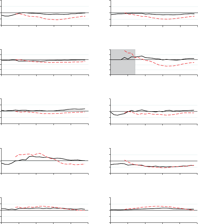
Figure 9. A comparison of the median responses of an anticipated (solid line) and unanticipated (dashed line)

government spending shock, where the impulses are plotted so that the time period of the implementation

of the increase in government spending is the same.

3.4. The Anticipated Government Revenue Shock

We also identify a year delayed shock where government revenue is restricted to rise only after a

year.

The responses of this shock are displayed in Figure 5. They show an intuitive ‘announcement

The zero restrictions for government revenue for the anticipated tax shock implicitly assume that, should GDP fall in

response to this announcement, taxes are temporarily raised to cover the associated decline in revenues during the year

before implementation (see Leeper et al. 2008). It should be noted that these implicit tax rises should be depressing

GDP further and yet the negative response of GDP is small and so this consideration does not go against our ﬁnding

 2009 John Wiley & Sons, Ltd. J. Appl. Econ. 24: 960–992 (2009)

DOI: 10.1002/jae

976 A. MOUNTFORD AND H. UHLIG

effect’ as the anticipated rise in revenues immediately depresses output and consumption. This

accords with our intuition regarding the optimal smoothing behavior of individuals and ﬁrms.

Interest rates also fall with this drop in output, which is also intuitive.

The median responses of the unanticipated and anticipated shocks are compared in Figure 6,

where the responses of the unanticipated shocks are shifted forward so that the implementation of

the revenue shock is in the same time period. Figure 6 shows that the responses to an anticipated

government revenue shock, while similar to those of the unanticipated shocks in terms of their

sign, are somewhat smaller, perhaps because announced policies move ﬁscal variables by less than

unanticipated changes.

3.5. The B asic Government Spending Shock

A basic government revenue shock is identiﬁed as a shock that is orthogonal to the business

cycle and monetary policy shock and where government spending rises for a year after the shock.

The identiﬁed government spending shocks are plotted in the fourth panel of Figure 1, where the

change from shaded to non-shaded areas denotes changes in presidential terms. These identiﬁed

shocks show that government spending shocks were predominantly positive in the mid 1960s and

early 1990s and predominantly negative around 1960 and in the early 1970s. In the the 1990s

government spending appears to be more stable than average, with relatively few shocks reaching

the 2.5% level in absolute terms.

The impulse responses for this shock are displayed in Figure 7. Figure 7 shows that the basic

government spending shock stimulates output during the ﬁrst four quarters, although only weakly,

and has only a very weak effect on private consumption. It also reduces investment, although

interestingly not via higher interest rates. Real wages do not respond positively to the government

spending shock and indeed are negative on impact and in the medium term, which is more in

accordance with neoclassical than New Keynesian models of government spending (see Ramey

and Shapiro, 1998). Although no restriction is placed on the behavior of government revenue, this

does not change very signiﬁcantly and so the basic government spending shock will resemble a

ﬁscal policy shock of deﬁcit spending, whose responses are displayed in Figure 10 below. The

response of prices to the increase in government spending is a little puzzling since both the

GDP deﬂator and the producer price index for crude materials show a decline. Although this is

a counter-intuitive result, it should be noted that this negative relationship between prices and

government spending has also been found in other studies (see, for example Canova and Pappa,

2007; Edelberg, et al., 1999. Fat

as and Mihov, 2001a).

that anticipated tax shocks have a much weaker response than unanticipated shocks. Further, note that an alternative

speciﬁcation for the anticipated tax shock, which places no restrictions on tax revenues for the year before implementation,

could easily be implemented.

When analyzing anticipated tax shocks, we implicitly assume that our VAR approach approximates a time series model,

in which news about tax shocks are always about the next annual tax change and not about subsequent ones. Otherwise,

overlapping news or a moving average process for taxes with two or more lags may result in problems with invertibility

and an appropriate VAR representation, as Leeper et al. (2008) have shown.

Changes in ﬁscal policy may be the result of the systematic component of ﬁscal policy—unrelated to the business

cycle— rather ﬁscal policy shocks, as Liu et al. (2007) have argued is the case for monetary policy shocks. However, we

leave the joint identiﬁcation of ﬁscal policy regime shifts and ﬁscal policy shock for future work.

 2009 John Wiley & Sons, Ltd. J. Appl. Econ. 24: 960–992 (2009)

DOI: 10.1002/jae

WHAT ARE THE EFFECTS OF FISCAL POLICY SHOCKS? 977

3.6. The Anticipated Government Spending Shock

We also identify a year delayed shock where government spending is restricted to rise only after

a year. The responses of this shock are displayed in Figure 8. They again show an intuitive

‘announcement’ effect on impact as the anticipated rise in spending immediately has a positive

effect on output and interest rates. Again this is consistent with smoothing behavior by individuals

and ﬁrms. The median responses of the unanticipated and anticipated shocks are compared

in Figure 9, where the responses of the unanticipated shocks are shifted forward so that the

implementation of the spending shock is in the same time period. Figure 9 shows that the responses

to an anticipated government spending shock appear more persistent and stronger than for the

unanticipated shocks and investment is no longer crowded out by the increase in government

spending. This is an interesting and slightly puzzling result; however, it should be noted that the

interpretation of these responses in the medium term is clouded by the marginal cut in taxes after

a year. From Figure 5 this would have a signiﬁcant expansionary effect and this may be the cause

of the persistent positive effects on income and consumption. In Section 4.1 below we demonstrate

a straightforward method for accounting for such changes when performing policy analysis.

4. POLICY ANALYSIS

We can use the basic shocks identiﬁed in the previous section to analyze the effects of different

ﬁscal policies. We view different ﬁscal policy shocks as different linear combinations of the basic

ﬁscal policy shocks. There are clearly a huge number of possible ﬁscal policies we could analyze,

so here we restrict ourselves to comparing three popularly analyzed ﬁscal policies. A deﬁcit-

spending shock, a deﬁcit ﬁnanced tax cut and a balanced budget spending shock. We ﬁrst detail

how the impulse responses for these policies are generated.

4.1. CALCULATING THE IMPULSE RESPONSES FOR DIFFERENT FISCAL POLICY

SCENARIOS

Our methodology regards different ﬁscal policy scenarios as being different combinations of the

two basic shocks over a sequence of several quarters. For example, a government spending scenario

where government spending is raised by 1% for four quarters while government revenue remains

unchanged is the linear combination of the sequence of the two basic shocks that generates these

responses in the ﬁscal variables as the combined impulse response. More formally, denoting r

j,a

k

as the response at horizon k of variable j to the impulse vector a, then the above policy requires

that

0.01 D



jD0

r

GS,BGS

k  jBGS

C r

GS,BGR

k  jBGR

 for k D 0,...K

0 D



jD0

r

GR,BGS

k  jBGS

C r

GR,BGR

k  jBGR

 for k D 0,...K

where K D 4, GS and GR stand for government expenditure and government revenue, and BGS

and BGR

are respectively the scale of the standard basic government spending and revenue shocks

in period j.

DOI: 10.1002/jae

978 A. MOUNTFORD AND H. UHLIG

-1

Percent

0 5 10 15 20 25

Quarters After the Shock

GDP

-1 -.5 0 .5

Percent

0 5 10 15 20 25

Quarters After the Shock

CONSUMPTION

-3 -2 -1 0 1 2

Percent

0 5 10 15 20 25

Quarters After the Shock

GOVERNMENT SPENDING

-6 -3 0 1 2

Percent

0 5 10 15 20 25

Quarters After the Shock

GOVERNMENT REVENUE

-1 -.5 0 .5 1

Percent

0 5 10 15 20 25

Quarters After the Shock

REAL WAGES

-4 -2 0 2 4

Percent

0 5 10 15 20 25

Quarters After the Shock

NON-RESIDENTIAL INVESTMENT

-.5 0 .5

Percent

0 5 10 15 20 25

Quarters After the Shock

INTEREST RATE

-2 -1 0 1 2

Percent

0 5 10 15 20 25

Quarters After the Shock

ADJUSTED RESERVES

-4 -2 0 2 4

Percent

0 5 10 15 20 25

Quarters After the Shock

PPIC

-1 -.5 0 .5 1

Percent

0 5 10 15 20 25

Quarters After the Shock

GDP DEFLATOR

.50-.5

Figure 10. The deﬁcit spending policy scenario where government spending is raised by 1% for four

quarters with government revenues remaining unchanged. These impulses are linear combinations of a

sequence of the basic shocks displayed in Figures 4 and 7. This ﬁgure is available in color online at

www.interscience.wiley.com/journal/jae

We analyze three key policy scenarios below: deﬁcit spending, a deﬁcit-ﬁnanced tax cut and a

balanced budget spending expansion. It should be clear, however, that other scenarios of interest

can be analyzed in this manner as well.

4.2. A Deﬁcit-Spending Fiscal Policy Scenario

The impulse responses for a deﬁcit spending ﬁscal policy scenario are shown in Figure 10. The

policy scenario is designed as a sequence of basic ﬁscal shocks such that government spending

DOI: 10.1002/jae

WHAT ARE THE EFFECTS OF FISCAL POLICY SHOCKS? 979

rises by 1% and tax revenues remain unchanged for four quarters following the initial shock.

As noted above, the standard basic government spending shock does not change tax revenues

signiﬁcantly, so the impulses in Figure 10 and are similar to those in Figure 7. Thus the deﬁcit

spending scenario stimulates output and consumption during the ﬁrst four quarters although only

weakly, it reduces non-residential investment and it produces a counter-intuitive response for

prices.

4.3. A Deﬁcit-Financed Tax Cut Fiscal Policy Scenario

The impulse responses for a deﬁcit ﬁnanced tax cut ﬁscal policy scenario are shown in Figure 11.

The policy scenario is designed as a sequence of basic ﬁscal shocks such that tax revenues fall by

1% and government spending remains unchanged for four quarters (including the initial quarter)

following the initial shock. The responses look very similar to a mirror image of the responses to

the basic government revenue shock in Figure 4. Thus the tax cut stimulates output, consumption

and investment signiﬁcantly, with the effect peaking after about 3 years. The effect on prices is

initially negative but subsequently positive following the rise in output.

4.4. The Balanced B udget Spending Policy Scenario

The balanced budget spending policy scenario is identiﬁed by requiring both government revenues

and expenditures to increase in such a way that the increase in revenues and expenditure is equal

for each period in the four-quarter window following the initial shock. For ease of comparison

we choose a sequence of basic ﬁscal shocks such that government spending rises by 1% and

government revenue rises by 1.28%. Government revenue rises by more than government spending

since over the sample government revenue’s share of GDP is 0.162, while that of government

spending is 0.208; thus we require government revenue to rise by (0.208/0.162)%. The results

are shown in Figure 12. These show that on impact there is a small expansionary effect on GDP

but thereafter the depressing effects of the tax increases dominate the spending effects, and GDP,

consumption and investment fall.

4.5. Measures of the Effects of Policy Scenarios

To compare the effects of one ﬁscal scenario with another it is useful to deﬁne summary measures

of the effects of each ﬁscal scenario. One measure used in the literature is the ratio of the response

of GDP at a given period to the initial movement of the ﬁscal variable (see, for example, Blanchard

and Perotti, 2002; Canova and Pappa, 2007). We refer to this as the impact multiplier. We report

the impact multipliers of the deﬁcit ﬁnanced tax cut and deﬁcit-spending policy scenarios below

in Tables III and IV.

However, we think a measure of the impact of a scenario along the entire path of the responses

up to a given period is also useful. In Figure 13 we have therefore plotted the present value of

the impulse responses of GDP and the ﬁscal variables for the deﬁcit-ﬁnanced tax cut and the

deﬁcit-spending policy scenarios. We have also calculated a present value multiplier for these

scenarios, which we display in Table II. To calculate the present value multiplier we use the

DOI: 10.1002/jae

980 A. MOUNTFORD AND H. UHLIG

-.5 0 .5 1

Percent

0 5 10 15 20 25

Quarters After the Shock

GDP

-.5 0 .5 1

Percent

0 5 10 15 20 25

Quarters After the Shock

CONSUMPTION

-3 -2 -1 0 1 2

Percent

0 5 10 15 20 25

Quarters After the Shock

GOVERNMENT SPENDING

-3 -2 -1 0 1 2

Percent

0 5 10 15 20 25

Quarters After the Shock

GOVERNMENT REVENUE

-1 -.5 0 .5 1

Percent

0 5 10 15 20 25

Quarters After the Shock

REAL WAGES

-4 -2 0 2 4

Percent

0 5 10 15 20 25

Quarters After the Shock

NON-RESIDENTIAL INVESTMENT

-.5 0 .5

Percent

0 5 10 15 20 25

Quarters After the Shock

INTEREST RATE

-2 -1 0 1 2

Percent

0 5 10 15 20 25

Quarters After the Shock

ADJUSTED RESERVES

-4 -2 0 2 4

Percent

0 5 10 15 20 25

Quarters After the Shock

PPIC

-1 -.5 0 .5 1

Percent

0 5 10 15 20 25

Quarters After the Shock

GDP DEFLATOR

Figure 11. The deﬁcit-ﬁnanced tax cut policy scenario where government spending remains unchanged

and government revenue is reduced by 1% for four quarters. These impulses are linear combinations of

a sequence of the basic shocks displayed in Figures 4 and 7. This ﬁgure is available in color online at

www.interscience.wiley.com/journal/jae

following formula:

Present value multiplier at lag k D



jD0

1 C i

j



jD0

1 C i

j

f/y

DOI: 10.1002/jae

WHAT ARE THE EFFECTS OF FISCAL POLICY SHOCKS? 981

-1.5 -1 -.5 0 .5

Percent

0 5 10 15 20 25

Quarters After the Shock

GDP

-1.5 -1 -.5 0 .5

Percent

0 5 10 15 20 25

Quarters After the Shock

CONSUMPTION

-3 -2 -1 0 1 2

Percent

0 5 10 15 20 25

Quarters After the Shock

GOVERNMENT SPENDING

-6 -3 0 1 2

Percent

0 5 10 15 20 25

Quarters After the Shock

GOVERNMENT REVENUE

-1 -.5 0 .5 1

Percent

0 5 10 15 20 25

Quarters After the Shock

REAL WAGES

-6 -4 -2 0 2 4

Percent

0 5 10 15 20 25

Quarters After the Shock

NON-RESIDENTIAL INVESTMENT

-.5 0 .5

Percent

Quarters After the Shock

INTEREST RATE

-2 -1 0 1 2

Percent

0 5 10 15 20 25

Quarters After the Shock

ADJUSTED RESERVES

-4 -2 0 2 4

Percent

0 5 10 15 20 25

Quarters After the Shock

PPIC

-1 -.5 0 .5 1

Percent

0 5 10 15 20 25

Quarters After the Shock

GDP DEFLATOR

Figure 12. The balanced budget policy scenario where government spending is raised by 1% for four quarters

and government revenues raised so that the increased revenue matches the increased spending. These impulses

are linear combinations of a sequence of the basic shocks displayed in Figures 4 and 7. This ﬁgure is available

in color online at www.interscience.wiley.com/journal/jae

where y

is the response of GDP at period j, f

is the response of the ﬁscal variable at period j,

i is the average interest rate over the sample, and f/y is the average share of the ﬁscal variable in

GDP over the sample. We use the median multiplier in all cases.

Table II and Figure 13 and tell the same story. They show that in present value terms tax cuts

have a much greater effect on GDP than government spending. The present value of the GDP

response to a deﬁcit spending scenario becomes insigniﬁcant after 2 years, whereas that for the

deﬁcit-ﬁnanced tax cut is signiﬁcantly positive throughout. Figure 13 also shows that the standard

DOI: 10.1002/jae

982 A. MOUNTFORD AND H. UHLIG

-2 0 2 4 6 8 10 12

Percent

0 5 10 15 20 25

Quarters After the Shock

DISCOUNTED CUMULATIVE GOVT SPENDING

-12 -9 -6 -3 0 1.5

Percent

0 5 10 15 20 25

Quarters After the Shock

DISCOUNTED CUMULATIVE GDP RESPONSES

DEFICIT SPENDING

-10 -5 0 5 10 15 20

Percent

0 5 10 15 20 25

Quarters After the Shock

DISCOUNTED CUMULATIVE GOVT REVENUE

-1 0 2 4 6 8 10 12

Percent

0 5 10 15 20 25

Quarters After the Shock

DISCOUNTED CUMULATIVE GDP RESPONSES

DEFICIT FINANCED TAX CUT

DISCOUNTED CUMULATIVE RESPONSES TO POLICY SHOCKS

Figure 13. The present value of the impulses for GDP and the changing ﬁscal variable for the deﬁcit-spending

policy scenario and the deﬁcit-ﬁnanced tax cut policy scenario displayed in Figures 10 and 11. This ﬁgure

is available in color online at www.interscience.wiley.com/journal/jae

Table II. Present value multipliers of the policy scenarios

1 qrt 4 qrts 8 qrts 12 qrts 20 qrts Maximum

Deﬁcit-ﬁnanced tax cut 0.29 0.52 1.63 5.25 4.55 5.25 (qrt 12)

Deﬁcit spending 0.65 0.46 0.07 0.26 2.07 0.65 (qrt 1)

This table shows the present value multipliers for a deﬁcit ﬁnanced tax cut policy scenario and for a deﬁcit-spending

ﬁscal policy scenario. The multipliers given are the median multipliers in both cases.

 2009 John Wiley & Sons, Ltd. J. Appl. Econ. 24: 960–992 (2009)

DOI: 10.1002/jae

WHAT ARE THE EFFECTS OF FISCAL POLICY SHOCKS? 983

error of the present value multiplier becomes very large for the deﬁcit-ﬁnanced tax cut at later

time periods.

4.6. Comparison of Results with the Existing Literature

Despite the novel methodology used in this paper, there are many similarities to results obtained

elsewhere in the existing literature. There are, however, also important differences, which we shall

discuss below. As we have used Blanchard and Perotti’s (2002) data deﬁnitions for the ﬁscal

variables and use a very similar sample period, it is natural to compare our results most closely

with their paper. We do this in the following subsection. We compare our results to other studies

in a further subsection.

4.6.1 Comparison with Blanchard and Perotti (2002)

The impact multipliers, deﬁned above, are compared with those of Blanchard and Perotti (2002)

in Tables III and IV.

For the deﬁcit-ﬁnanced tax cut, Table III shows that our results are very comparable with

Blanchard and Perotti’s. In both studies the effect on output of a change in tax revenues is

persistent and large. The size of the impact multiplier is greater in our results than in Blanchard

and Perotti’s, although in both studies the impact multipliers of the tax cut scenario are greater

than those of the spending scenario.

For the spending scenario, Table IV shows that size of the impact multipliers associated with

increased government spending is smaller than Blanchard and Perotti’s, but that the timing has a

similar pattern in the sense that the largest impact multipliers are in the periods close to the impact

of the initial shock and with the responses after a year being insigniﬁcant.

With respect to the responses of investment again the two studies are similar. In both Blanchard

and Perotti’s and in our study investment falls in response to both tax increases and government

Table III. Impact multipliers of deﬁcit-ﬁnanced tax cut policy scenarios

1 qrt 4 qrts 8 qrts 12 qrts 20 qrts Maximum

Mountford and Uhlig

GDP 0.28 0.93 2.05 3.41 2.59 3.57 (qrt 13)

Tax revenues 1.00 1.00 0.06 1.05 1.03

Gov. spending 0.00 0.00 0.27 0.43 0.48

Blanchard and Perotti

(2002)

GDP 0.70 1.07 1.32 1.30 1.29 1.33 (qrt 7)

Tax revenues 0.74 0.31 0.17 0.16 0.16

Gov. spending 0.06 0.10 0.17 0.20 0.20

This table shows the impact multipliers for a deﬁcit-ﬁnanced tax cut ﬁscal scenario for various quarters after the initial

shock and compares them to similar measures from Blanchard and Perotti (2002 Table III). The multiplier represents the

effect in dollars of a one-dollar cut in taxes at the ﬁrst quarter. For the Mountford and Uhlig results this is calculated

with the formula: Multiplier for GDP D

GDP response

Initial ﬁscal shock

/(Average ﬁscal variable share of GDP), where the median

responses are used in all cases. On the calculation of the Blanchard and Perotti (2002) multipliers see Blanchard and

Perotti (2002 section V).

The median multiplier becomes negative at later time periods for both the deﬁcit spending and deﬁcit-ﬁnanced tax cut

shocks but in both cases these negative multipliers are not signiﬁcant.

 2009 John Wiley & Sons, Ltd. J. Appl. Econ. 24: 960–992 (2009)

DOI: 10.1002/jae

984 A. MOUNTFORD AND H. UHLIG

Table IV. Impact multipliers of a deﬁcit-spending policy scenario

1 qrt 4 qrts 8 qrts 12 qrts 20 qrts Maximum

Mountford and Uhlig

GDP 0.65 0.27 0.74 1.19 2.24 0.65 (qrt 1)

Gov. spending 1.00 1.00 0.90 0.37 0.32

Tax revenues 0.00 0.00 0.33 0.87 2.04

Blanchard and Perotti

(2002)

GDP 0.90 0.55 0.65 0.66 0.66 0.90 (qrt 1)

Gov. spending 1.00 1.30 1.56 1.61 1.62

Tax revenues 0.10 0.18 0.33 0.36 0.37

This table shows the impact multipliers for a deﬁcit-spending ﬁscal scenario for various quarters after the initial shock

and compares them to similar measures from Blanchard and Perotti (2002 Table IV). The multiplier represents the effect

in dollars of a one-dollar increase in spending at the ﬁrst quarter. For the Mountford and Uhlig results this is calculated

with the formula: Multiplier for GDP D

GDP response

Initial ﬁscal shock

/(Average ﬁscal variable share of GDP), where the median

responses are used in all cases. On the calculation of the Blanchard and Perotti (2002) multipliers see Blanchard and

Perotti (2002 section V).

spending increases. With regard to consumption the results have some similarities to Blanchard and

Perotti’s in that consumption does not fall in response to a spending shock. However, in Blanchard

and Perotti (2002) consumption rises signiﬁcantly in response to a spending shock, whereas in our

analysis consumption does not move by very much.

As Figure 10 shows, consumption’s response

is only signiﬁcantly positive on impact and then by only a small amount. Thereafter its response is

insigniﬁcant. Finally, we ﬁnd that real wages do not rise in response to an increase in government

spending and have a negative response on impact and at longer horizons. Thus, taken together,

these ﬁndings are difﬁcult to reconcile with the standard Keynesian approach, although they are

also not the responses predicted by the benchmark real business cycle model.

4.6.2 Comparison with Other Studies

With regard to other studies in the literature, not only are there differences in methodology but

also in the deﬁnitions of the ﬁscal variables. There is thus no shortage of potential sources for

differences in results. Nevertheless, there is still some common ground in the results of this paper

and previous work. For example, consider the recent work by Burnside et al. (2003), which builds

on the work of Ramey and Shapiro (1998) and Edelberg et al. (1999) in using changes in military

purchases associated with various wars to identify government spending shock. They ﬁnd that

private consumption does not change signiﬁcantly in response to a government spending shock.

However, in contrast to our results they ﬁnd that investment has an initial, transitory positive

response to the spending shock.

4.7. Variance of the Policy Analysis

Clearly there is a considerable degree of uncertainty in the numbers displayed in Tables III and IV,

as they are based on the maximum multipliers from the median impulse responses. An advantage

of the Bayesian approach used in our analysis is that it naturally provides a measure of the standard

See also Gali et al. (2007), who also ﬁnd a signiﬁcantly positive consumption response.

 2009 John Wiley & Sons, Ltd. J. Appl. Econ. 24: 960–992 (2009)

DOI: 10.1002/jae

WHAT ARE THE EFFECTS OF FISCAL POLICY SHOCKS? 985

errors for this policy analysis. Standard errors can easily be calculated for each policy scenario by

taking the maximum and minimum multipliers of GDP and their corresponding lag for each of

the draws from the posterior. These maxima and minima can then be ordered and the 16th, 50th

and 84th percentiles reported. This is done in Table V.

Table V supports the conclusions above. The maximum expansionary effect of a deﬁcit-spending

scenario is much below that of the tax revenue scenario. Indeed the upper conﬁdence limit of the

deﬁcit-spending scenario is below the lower conﬁdence limit of the tax cut scenario. For the tax

cut the maximum effects are signiﬁcantly positive and the minimum effects are insigniﬁcantly

different from zero.

The results in Table V are usefully related to the impulse responses in Figures 10–12. For

the tax cut the maximum multipliers occur after two or more years, whereas for the balanced

budget and deﬁcit-spending scenarios the maximum effects occur at short lags and the minimum

effects at longer lags. Since the variance of the impulse responses for these scenarios appears to

increase at longer lag lengths, we also look at the maximum and minimum multipliers of the two

spending scenarios in the ﬁrst year after the initial shock. In this case we now get the result that

the deﬁcit-spending scenario’s minimum multiplier is insigniﬁcantly different from zero but that

for the balanced budget spending scenario is still signiﬁcantly negative.

These statistics relate to the distribution of the maximum and minimum impact multiplier

effects of each ﬁscal scenario. For each draw the maximum and minimum ﬁscal multiplier is

calculated and the 16th, 50th and 84th percentiles of these results are displayed. The multiplier

statistic is calculated in terms of the initial, lag 0, ﬁscal shock as follows: multiplier for

GDP D

GDP response

Fiscal shock at Lag 0

/(Average ﬁscal variable share of GDP).

4.8. Policy Conclusions

An important lesson one can draw from the results is that while a deﬁcit-ﬁnanced expenditure

stimulus is possible, the eventual costs are likely to be much higher than the immediate beneﬁts.

Suppose that government spending is increased by 2%, ﬁnanced by increasing the deﬁcit: this

results, using the median values from Table V, at maximum, in less than a 2% increase in GDP. But

the increased deﬁcit needs to be repaid eventually with a hike in taxes. Even ignoring compounded

Table V. Maximum and minimum impact multipliers of ﬁscal policy scenarios

Fiscal scenario Maximum multiplier Minimum multiplier

Median

multiplier

Conﬁdence interval

16th, 84th quantiles

Median

multiplier

Conﬁdence interval

16th, 84th quantiles

Deﬁcit spending 0.91 0.68, 1.37 2.88 4.99, 0.80

lag 4 lag 2, lag 6 at lag 20 lag 24, lag 8

Balanced budget 0.47 0.19, 0.84 5.84 9.46, 3.63

lag 1 lag 1, lag 1 at lag 19 lag 15, lag 11

Tax cut 3.81 2.58, 5.49 0.19 0.11, 0.36

lag 12 lag 15, lag 13 at lag 24 lag 24, lag 1

Deﬁcit spending 0.79 0.59, 1.05 0.09 0.21, 0.31

in ﬁrst year lag 4 lag 4, lag 1 at lag 4 lag 4, lag 2

Balanced budget 0.45 0.16, 0.79 0.71 1.11, 0.40

in ﬁrst year at lag 3 lag 1, lag 1 at lag 4 lag 1, lag 2

DOI: 10.1002/jae

986 A. MOUNTFORD AND H. UHLIG

interest rates, this would require a tax hike of over 2%.

This tax hike results in a greater than

7% drop in GDP. Thus, unless the policy maker’s discount rate is very high, the costs of the

expansion will be much higher than the initial beneﬁt.

This general line of reasoning is consistent with the balanced budget spending scenario

whose impulses are shown in Figure 12. This shows that when government spending is ﬁnanced

contemporaneously the contractionary effects of the tax increases outweigh the expansionary effects

of the increased expenditure after a very short time.

5. CONCLUSION

In this paper we have presented a new approach for distinguishing the effects of ﬁscal policy

shocks by adapting the method of Uhlig (2005). This method uses only the information in the

macroeconomic time series of the vector autoregression together with minimal assumptions to

identify ﬁscal policy shocks. In particular, it imposes no restrictions on the signs of the responses

of the key variables of interest—GDP, private consumption, real wages and private non-residential

investment—to ﬁscal policy shocks. The paper applied this approach using post-war data on the

US economy.

We have analyzed three types of policy scenarios: a deﬁcit-ﬁnanced spending increase, a

balanced budget spending increase (ﬁnanced with higher taxes) and a deﬁcit-ﬁnanced tax cut,

in which revenues increase but government spending stays unchanged. We found that a deﬁcit-

spending scenario stimulates the economy for the ﬁrst four quarters but only weakly compared

to that for a deﬁcit-ﬁnanced tax cut. We also found that both types of spending scenario had the

effect of crowding out investment.

Although the best ﬁscal policy for stimulating the economy appears to be deﬁcit-ﬁnanced tax

cuts, we wish to point out that this should not be read as endorsing them. This paper only points

out that unanticipated deﬁcit-ﬁnanced tax cuts work as a (short-lived) stimulus to the economy,

not that they are sensible. The resulting higher debt burdens may have long-term consequences

which are far worse than the short-term increase in GDP, and surprising the economy may not

be good policy in any case. These normative judgements require theoretical models for which the

empirical positive results in this paper can provide a useful starting point.

ACKNOWLEDGEMENTS

This paper is a substantially revised version of the CEPR discussion paper No 3338. This research

has been sponsored by the Deutsche Forschungsgemeinschaft through the SFB 649 ‘Economic

Risk’ and by the RTN networks NASEF and MAPMU. We are grateful to comments by seminar

audiences at Royal Holloway, Exeter University, Milan, an NASEF meeting on Hydra, an SFB 373

meeting in Wulkow, a conference in Alicante, Southampton University and the London Business

School. Special thanks go to Greg Mankiw for pointing out an important issue in an earlier version

of this paper, which we have now resolved.

For simplicity, we are assuming the tax hike to be a surprise, when it occurs, which allows us to use the results above.

 2009 John Wiley & Sons, Ltd. J. Appl. Econ. 24: 960–992 (2009)

DOI: 10.1002/jae

WHAT ARE THE EFFECTS OF FISCAL POLICY SHOCKS? 987

REFERENCES

Beaudry P, Portier F. 2003. Stock prices, news and economic ﬂuctuations. Mimeo, University of Toulouse.

Benati L, Mumtaz H. 2007. US evolving macroeconomic dynamics: a structural investigation. Working Paper

Series No. 746, European Central Bank.

Bernanke BS. 1986. Alternative explanations of the money–income correlation. In Real Business Cycles,

Real Exchange Rates, and Actual Policies, Brunner K, Meltzer A (eds). Carnegie-Rochester Conference

Series on Public Policy, no. 25. North-Holland: Amsterdam.

Bernanke BS, Mihov I. 1998. Measuring monetary policy. Quarterly Journal of Economics 113(3): 869–890.

Blanchard O. 1997. Macroeconomics. Prentice-Hall: Englewood Cliffs, NJ.

Blanchard O, Perotti R. 2002. An empirical characterization of the dynamic effects of changes in government

spending and taxes on output. Quarterly Journal of Economics. 117(4): 1329–1368.

Blanchard OJ, Quah D. 1989. The dynamic effects of aggregate demand and supply disturbances. American

Economic Review 79(September): 655–673.

Blanchard O, Watson M. 1986. Are all Business cycles alike? In R.J. Gordon, ed., The American Business

Cycle, Gordon RJ (ed.). University of Chicago Press: Chicago, IL; 123–160.

Burnside C, Eichenbaum M, Fisher JDM. 2003. Fiscal shocks and their consequences. Working Paper 9772,

National Bureau of Economic Research.

Canova F, De Nicol

o G. 2002. Monetary disturbances matter for business ﬂuctuations in the G7. Journal of

Monetary Economics 49: 1131–1159.

Canova F, De Nicol

o G. 2003. On the sources of business cycles in the G7. Journal of International

Economics 59: 77–100.

Canova F, Pappa E. 2007. Price differentials in monetary unions: the role of ﬁscal shocks. Economic Journal

117: 713–737.

Canova F, Pina J. 1998. Monetary policy misspeciﬁcation in VAR models. Working paper, CEPR.

Christiano LJ, Eichenbaum M, Evans C. 1999. Monetary policy shocks: what have we learned and to what

end? Handbook of Monetary Economics, Woodford M, Taylor J (eds). Northwestern University: Evanston,

IL.

Chung H, Leeper EM. 2007. What has ﬁnanced government debt? Working Paper No. W13425, NBER.

Cochrane JH. 1994. Permanent and transitory components of GNP and stock prices. Quarterly Journal of

Economics 109(1): 241–265.

Dedola L, Neri S. 2007. What does a technology shock do? A VAR analysis with model-based sign

restrictions. Journal of Monetary Economics 54(2): 512–549.

Devereux MB, Head AC, Lapham M. 1996. Monopolistic competition, increasing returns and the effects of

government spending. Journal of Money, Credit and Banking 28: 233–254.

Dungey M, Fry R. 2007. The identiﬁcation of ﬁscal and monetary Policy in a structural VAR. M, Wo rking

Paper No. 29–2007, CAMA.

Edelberg W, Eichenbaum M, Fisher JDM. 1999. Understanding the effects of a shock to government

purchases. Review of Economic Dynamics 2: 166–206.

Eichenbaum M, Fisher JDM. 2004. Fiscal policy in the aftermath of 9/11. Working Paper 32704,Northwest-

ern University.

Fat

as A, Mihov I. 2001a. Fiscal policy and business cycles: an empirical investigation. Moneda y Credito

212: 167–210.

Fat

as A, Mihov I. 2001b. The effects of ﬁscal policy on consumption and employment: theory and evidence.

Draft, INSEAD.

Faust J. 1998. On the robustness of the identiﬁed VAR conclusions about money. Carnegie Rochester

Conference Series on Public Policy 49: 207–244.

Favero C. 2001. Applied Macroeconometrics. Oxford University Press: Oxford.

Favero C. 2002. How do European monetary and ﬁscal authorities behave? Draft, IGIER, Bocconi University.

Fry R, Pagan A. 2007. Some issues in using sign restrictions for identifying structural VARs. Working Paper

No. 14, NCER.

Gal

ı J. 1992. How well does the IS-LM model ﬁt postwar US data? Quarterly Journal of Economics 107(2):

709–738.

Gal

ıJ,L

opez-Salido JD, Vall

es J. 2007. Understanding the effects of government spending on consumption.

Journal of the European Economic Association 5(1): 227–270.

DOI: 10.1002/jae

988 A. MOUNTFORD AND H. UHLIG

Giavazzi F, Jappelli T, Pagano M. 1990. Can severe ﬁscal contractions be expansionary? Tales of two

small European countries. In NBER Macroeconomics Annual, Blanchard OJ, Fisher S (eds). MIT Press:

Cambridge, MA; 75 –110.

Giavazzi F, Pagano M. 2000. Searching for non-linear effects of ﬁscal policy: evidence from industrial and

developing countries. European Economic Review 44: 1259 –1289.

Hemming R, Kell M, Mahfouz S. 2000. The effectiveness of ﬁscal policy in stimulating economic activity:

a review of the literature. Mimeo, International Monetary Fund.

Leeper E, Sims C, Zha T. 1996. What does monetary policy do? Brookings Papers on Economic Activity. 2:

1–63.

Leeper E, Walker TB, Yang S-CS. 2008. Fiscal foresight: analytics and econometrics. Mimeo, Indiana

University.

Liu Z, Waggoner DF, Zha T. 2007. Expectation effects of regimes shifts in monetary policy. Kiel Wo rking

Papers 1357, Kiel Institute for the World Economy.

Mountford A, Uhlig H. 2002. What are the effects of ﬁscal policy shocks? Discussion Papers No. 3338,

CEPR.

Mountford A. 2005. Leaning into the wind: a structural VAR investigation of UK monetary policy. Oxford

Bulletin of Economics and Statistics 67(5): 597–621.

Peersman G. 2005. What caused the early millennium slowdown? Evidence based on vector autoregression.

Journal of Applied Econometrics 20(2): 185–207.

Perotti R. 1999. Fiscal policy in good times and bad. Quarterly Journal of Economics. 114(4): 1399–1436.

Ramey V, Shapiro M. 1998. Costly capital reallocation and the effects of government spending. In Carnegie

Rochester Conference on Public Policy.

Romer DH, Romer C. 1994. What ends recessions? NBER Macroeconomics Annual 9: 13–57.

Romer DH, Romer C. 2007. The macroeconomic effects of tax changes: estimates based on a new measure

of ﬁscal shocks. Working Paper No. 13264 , NBER.

Sims CA. 1986. Are forecasting models usable for policy analysis? Minneapolis Federal Reserve Bank

Quarterly Review Winter: 2 –16.

Sims CA, Zha T. 1998. Bayesian methods for dynamic multivariate models. International Economic Review

39(4): 949–968.

Trabandt M, Uhlig H. 2006. How far are we from the slippery slope? The Laffer curve revisited. SFB 649

Discussion Paper No. 2006-023.

Uhlig H. 2005. What are the effects of monetary policy? Results from an agnostic identiﬁcation procedure.

Journal of Monetary Economics 52: 381–419.

APPENDIX A: VARS AND IMPULSE MATRICES

A VAR in reduced form is given by



iD1

ti

C u

,t D 1,....T, E[u

] D 

where Y

are m ð 1vectors,L is the lag length of the VAR, B

are m ð m coefﬁcient matrices and

is the one-step-ahead prediction error.

The problem of identiﬁcation is to translate the one-step-ahead prediction errors, u

,into

economically meaningful, or ‘fundamental’, shocks,

. We adopt the common assumptions in the

VAR literature that there are m fundamental shocks, which are mutually orthogonal and normalized

to be of variance 1. Thus E[

] D I

. Identiﬁcation of these shocks amounts to identifying a

matrix A, such that u

D Av

and AA

D .Thejth column of A represents the immediate impact,

or impulse vector, of a one standard error innovation to the jth fundamental innovation, which is

the jth element of

v. The following deﬁnition is useful, and new.

DOI: 10.1002/jae

WHAT ARE THE EFFECTS OF FISCAL POLICY SHOCKS? 989

Deﬁnition 1 An impulse matrix of rank n is a n ð m sub-matrix of some m ð m matrix A, such

that AA

D . An impulse vector a is an impulse matrix of rank 1, i.e., a vector a 2 

such that

there exists some matrix A, where a is a column of A, such that AA

D .

One can show that the identiﬁcation does not depend on the particular matrix A chosen beyond

a given impulse matrix, i.e., a given impulse matrix uniquely identiﬁes the fundamental shocks

corresponding to it.

Theorem 1 Suppose that  is regular. Let a given impulse matrix [a

1

,...,a

n

] of size n be

a submatrix of two m ð m matrices A,

A with AA

D .Letv

D A

1

, Qv

1

and let

1

,...,v

n

resp. Qv

1

,...,Qv

n

be the entries in v

resp. Qv

corresponding to a

1

,...,a

n

, i.e., if,

for example, a

1

is the third column of A, then v

1

is the third entry of v

. Then, v

i

DQv

i

for all

i D 1,...,n.

Proof Without loss of generality, let [a

1

,...,a

n

]betheﬁrstn columns of A and

A.Ifthisis

for example, not the case for A and if, for example, a

1

is the third column of A, one can ﬁnd

a permutation matrix P so that the given impulse matrix will be the ﬁrst n columns of

A D AP

with a

1

the ﬁrst column of

A.SincePP

D I,

D . Furthermore, the ﬁrst column of P is

the vector e

, which is zero except for a 1 in its third entry: hence the ﬁrst entry of

1

D P

must be the third entry of v

and thus be v

1

corresponding to a

1

With [a

1

,...,a

n

]astheﬁrstn columns of A and

A,letE

D [I

, 0

n,m

]. Note that

[

1

,...,v

n

]

D E

1

.WeneedtoshowthatE

1

D E

1

for all u

.Itsufﬁcesto

show that E

1

 D E

1

,since is regular. But this follows from

1

 D E

1

D E

D [a

1

,...,a

n

]

D E

1

D E

1





In the VAR literature identiﬁcation usually proceeds by identifying all m fundamental shocks

and so characterizing the entire A matrix. This requires imposing mm  1/2 restrictions on the

A matrix. This is done either by assuming a recursive ordering of variables in the VAR, so that

a Cholesky decomposition of A can be used (see Sims, 1986), or by imposing the mm  1/2

restrictions via assumed short-run structural relationships as in Bernanke (1986) and Blanchard and

Watson (1986), via assumed long-run structural relationships, as in Blanchard and Quah (1989) or

via both assumed short-run and long-run structural relationships as in Gal

ı (1992).

This paper instead extends the method of Uhlig (2005) and identiﬁes at most three fundamental

shocks and so needs to characterize an impulse matrix [a

1

2

3

] of rank 3 rather than all

of A. This is accomplished by imposing sign restrictions on the impulse responses. Note that, by

construction, the covariance between the fundamental shocks

1

, v

2

and v

3

corresponding to

1

2

and a

3

is zero, i.e., that these fundamental shocks are orthogonal.

DOI: 10.1002/jae

990 A. MOUNTFORD AND H. UHLIG

To that end, note that any impulse matrix [a

1

,...,a

n

] can be written as the product

1

,...,a

n

] D

AQ of the lower triangular Cholesky factor

A of  with an n ð m matrix

Q D [q

1

,...,q

n

] of orthonormal rows q

i

, i.e., QQ

D I

: this follows from noting that

1

A must be an orthonormal matrix for any decomposition AA

D  of . Likewise, Let

a D a

s

,s 2f1,...,ng be one of the columns of the impulse matrix and q D q

s

1

s

the corresponding column of Q: note that q

s

does not depend on the other a

p

,p 6D s.Asin

Uhlig (2005), it follows easily that the impulse responses for the impulse vector a can be written

as a linear combination of the impulse responses to the Cholesky decomposition of  as follows.

Deﬁne r

k as the impulse response of the jth variable at horizon k to the ith column of

A,and

the m-dimensional column vector r

k as [r

k,...,r

k]. Then the m-dimensional impulse

response r

k at horizon k to the impulse vector a

s

is given by

k D



iD1

k 1

(where q

is the ith entry of q D q

s

Deﬁne the function f on the real line per fx D 100x if x ½ 0andfx D x if x  0. Let s

the the standard error of variable j.LetJ

S1C

be the index set of variables for which identiﬁcation

of a given shock restricts the impulse response to be positive and let J

S1

be the index set of

variables for which identiﬁcation restricts the impulse response to be negative. To impose the

additional identifying inequality sign restrictions beyond the zero restrictions of equation (3), we

solve

a D argmin

a 2

where the criterion function a is given by

a D



jεJ

S,C



kD0





k





jεJ

S,



kD0



k



Computationally, we implement this minimization using a simplex algorithm: it is available

on many statistical packages, such as MATLAB and RATS; for this paper we use the version

of the algorithm written in GAUSS by Bo Honore and Ekaterini Kyriazidou, available from

http://webware.princeton.edu/econometrics/programs/gaussmax/

Note that ‘zero’ restrictions, where the impulse responses of the jth variable to an impulse

vector a for, say, the ﬁrst four periods are set to zero, can be incorporated into the analysis fairly

easily. These restrictions can be written as a restriction on the vector q that

0 D Rq 3

where R is a 4 ð m matrix of the form

R D







0 ÐÐÐ r

0

3 ÐÐÐ r

3







4

DOI: 10.1002/jae

WHAT ARE THE EFFECTS OF FISCAL POLICY SHOCKS? 991

To identify an impulse matrix [a

1

2

], where the ﬁrst shock is a business cycle shock and

the second shock is a ﬁscal policy shock, ﬁrst identify the business cycle shock a

1

the manner described above and then identify the second shock a

2

by replacing the minimization

problem (2) with

a D argmin

Aq,RqD0,q

1

a 5

i.e., by additionally imposing orthogonality to the ﬁrst shock. The two restrictions Rq D 0,q

1

0 can jointly be written as

0 D

Rq 6

where

D [q

1

]. Likewise, if orthogonality to two shocks— the business cycle shock and the

monetary policy shock—is required, identify the business cycle shock a

1

and identify

the monetary policy shock a

2

and solve

a D argmin

Aq,RqD0,q

1

2

a 7

Given the above we can now state our identiﬁcation restrictions more formally. We only provide

two: the others follow the same pattern.

Deﬁnition 2 A business cycle shock impulse vector is an impulse vector a that minimizes a

criterion function a, which penalizes negative impulse responses of GDP, private consumption,

non-residential investment and government revenue at horizons k D 0,1,2,and3.

Deﬁnition 3 A basic government revenue shock impulse vector is an impulse vector a minimizing

a criterion function a, which penalizes negative impulse responses to the vector a of government

revenue at horizons k D 0, 1, 2, and 3.

The computations are performed using a Bayesian approach as in Uhlig (2005) (see also Sims

and Zha, 1998). We take a number of draws from the posterior. For each draw from the posterior

of the VAR coefﬁcients and the variance–covariance matrix , the shocks are identiﬁed using the

criteria described above. Given the sample of draws for the impulse responses, conﬁdence bands

can be plotted.

APPENDIX B: THE DATA

All the data we use are freely available from the World Wide Web. The data on components

of US national income is taken from the National Income and Product Accounts (NIPA),

which are made publically available by the Bureau of Economic Analysis on their website

http://www.bea.gov/national/nipaweb/index.asp/. The monetary data—the interest rate, producer

commodity price index and adjusted reserves—and the real wage data are taken from the Federal

Reserve Board of St Louis website http://www.stls.frb.org/fred/.

7.1. B.1. Deﬁnitions of Variables in the VAR

All the components of national income are in real per capita terms and are transformed from their

nominal values by dividing them by the gdp deﬂator (NIPA Table VII.1, row 4) and the population

DOI: 10.1002/jae

992 A. MOUNTFORD AND H. UHLIG

measure (NIPA Table II.1, row 35). The table and row numbers refer to the organization of the

data by the Bureau of Economic Analysis.

GDP: This is NIPA Table I.1, row 1.

Private Consumption: This is NIPA Table I.1, row 2.

Total Government Expenditure: This is ‘Federal Defense Consumption Expenditures’, NIPA

Table III.7 row 4, plus ‘Federal Non Defense Consumption Expenditures’, NIPA Table III.7,

row 15, plus ‘State and Local Consumption Expenditures’, NIPA Table III.7, row 28. plus

‘Federal Defense Gross Investment’, NIPA Table III.7, row 11, plus ‘Federal Non Defense Gross

Investment’, NIPA Table III.7, row 24, plus ‘State and Local Gross Investment’, NIPA Table III.7,

row 35.

Total Government Revenue:

This is ‘Total Government Receipts’, NIPA Table III.1, row 1,

minus ‘Net Transfers Payments’, NIPA Table III.1, row 8, and ‘Net Interest Paid’, NIPA Table III.1

row 11.

Real Wages: This is ‘Nonfarm Business Sector: Real Compensation Per Hour’ Series COMPRNFB

from the US Department of Labor: Bureau of Labor Statistics.

Private Non-Residential Investment: This is ‘Nominal Gross Private Domestic Investment’,

NIPA Table I.1, row 6, minus private residential investment, NIPA Table I.1, row 11.

Interest Rate: This is the Federal Funds rate which is the series fedfunds at the Federal Reserve

Board of St Louis website http://www.stls.frb.org/fred/. We take the arithmetic average of the

monthly ﬁgures for the Federal Funds Rate.

Adjusted Reserves: This is the Adjusted Monetary Base given by the series adjressl at the Federal

Reserve Board of St Louis website http://www.stls.frb.org/fred/. We take the arithmetic average

of the monthly ﬁgures to get a quarterly ﬁgure.

PPIC: This is the Producer Price Index of Crude Materials given by the series ppicrm at the

Federal Reserve Board of St Louis website http://www.stls.frb.org/fred/. We take the arithmetic

average of the monthly ﬁgures to get a quarterly ﬁgure.

The GDP Deﬂator: This is NIPA Table VII.1, row 4.

The VAR system consists of these 10 variables at quarterly frequency from 1955 (Q1) to 2000

(Q4), has six lags, no constant or time trend, and uses the logarithm for all variables except the

interest rate where we have used the level.

The ﬁscal variables are chosen so that they will have different responses to business cycle

movements and ﬁscal policy shocks. The government expenditure variable is chosen so as to

exclude expenditures which will vary over the business cycle such as transfer payments; see,

for example, Blanchard (1997, p. 600) on this. The government receipts variable should clearly

respond positively to a business cycle shock; an increase in output should increase tax receipts

and reduce transfer payments.

This deﬁnition follows Blanchard and Perotti (2002) regarding transfer payments as negative taxes. We use this deﬁnition

in order not to obscure the implications of the new identiﬁcation technique used in this paper, by using different data.

 2009 John Wiley & Sons, Ltd. J. Appl. Econ. 24: 960–992 (2009)

DOI: 10.1002/jae