Macroeconomic Stability in Resource-Rich Countries: The Role of Fiscal Policy; by Elva Bova, Paulo Medas, and Tigran Poghosyan; IMF Working Paper WP/16/36; February 2016

WP/16/36

Macroeconomic Stability in Resource-Rich Countries:

The Role of Fiscal Policy

by Elva Bova, Paulo Medas, and Tigran Poghosyan

IMF Working Paper

Fiscal Affairs Department

Resource Revenue Volatility and Macroeconomic Stability in Resource-Rich Countries:

The Role of Fiscal Policy

Prepared by Elva Bova, Paulo Medas, and Tigran Poghosyan

Authorized for distribution by Bernardin Akitoby

February 2016

Abstract

Resource-rich countries face large and persistent shocks, especially coming from volatile

commodity prices. Given the severity of the shocks, it would be expected that these countries

adopt countercyclical fiscal policies to help shield the domestic economy. Taking advantage

of a new dataset covering 48 non-renewable commodity exporters for the period 1970-2014,

we investigate whether fiscal policy does indeed play a stabilizing role. Our analysis shows

that fiscal policy tends to have a procyclical bias (mainly via expenditures) and, contrary to

others, we do not find evidence that this bias has declined in recent years. Adoption of fiscal

rules does not seem to reduce procyclicality in a significant way, but the quality of political

institutions does matter. Finally, non-commodity revenues tend to respond only to persistent

changes in commodity prices.

JEL Classification Numbers: O13, H30, C33

Keywords: commodity prices, resource-rich countries, procyclical fiscal policy

Author’s E-Mail Address: [email protected], [email protected], [email protected].

This working paper draws on the analysis done for the Fiscal Monitor (IMF 2015a). The authors thank IMF

colleagues for useful comments and suggestions. Tafadzwa Mahlanganise provided research assistance. The

usual disclaimer applies.

IMF Working Papers describe research in progress by the author(s) and are published to elicit

comments and to encourage debate. The views expressed in IMF Working Papers are those of the

author(s) and do not necessarily represent the views of the IMF, its Executive Board, or IMF

management.

Content Page

Abstract ................................................................................................................................................................................. 2



I. Introduction ......................................................................................................................................................... 4

II. Related Literature .............................................................................................................................................. 5

III. The Size and Impact of Commodity Price Fluctuations ...................................................................... 6 

IV. Fiscal Cyclicality .................................................................................................................................................. 9

A. Measure 1: Commodity prices and government spending .......................................................... 9

B. Measure 2: The cyclically-adjusted non-resource balance ........................................................ 11

C. Can institutions help reduce procyclicality? .................................................................................... 12

V. How Do Non-Resource Revenues Respond to Commodity Revenue Shocks? ...................... 16

VI. Conclusions ....................................................................................................................................................... 17

Annex 1. Data ................................................................................................................................................................... 18

References ......................................................................................................................................................................... 26

Tables

1. Descriptive statistics: Commodity price growth rates ...................................................................... 19



2. Duration of commodity price expansions and contractions .......................................................... 20

3. Amplitude of commodity price expansions and contractions ...................................................... 21

4. Estimation results: Government spending and commodity prices .............................................. 22

5. Estimation results: Non-commodity output gap and cyclically-adjusted non-commodity

balance ................................................................................................................................................................ 22



6. Impact of fiscal rules on fiscal procyclicality ........................................................................................ 23

7. Impact of institutions on fiscal procyclicality ....................................................................................... 23

8. Impact of commodity revenue shocks on non-commodity revenues ....................................... 24

9. Resource funds and rules ............................................................................................................................ 25

Figures

1. Impact of commodity price swings on fiscal revenues and exports .............................................. 7



2. The 1970s-80s boom and bust had a long-lasting negative impact on growth for

commodity exporting countries .................................................................................................................. 8



3. The degree of procyclicality appears to have been stable over time......................................... 11

4. Institutional quality in resource-rich countries is weaker than in other countries ................ 15

I. INTRODUCTION

The recent dramatic turnaround in energy prices once again shifted the attention of policymakers

to commodity price shocks and their impact on macroeconomic stability in resource-rich

countries. Movements in commodity prices affect these economies directly through the external

trade balance (commodity exports) and the public sector budget (governments receive a large

share of commodity sector revenues). There are also indirect channels, such as changes in

borrowing conditions, asset prices, and investment. Given the high dependence on budgetary

commodity revenues and exports, the large price fluctuations imply these countries are exposed

to large external risks.

A key policy objective for resource-rich countries is to shield the economy from the high volatility

of commodity prices. The traditional advice is for countries to develop stabilizing

(countercyclical) fiscal policies towards helping smooth the business cycle (IMF 2015b). This is a

more complex and critical challenge for non-renewable resource-rich economies. A central issue

is that the economic cycle tends to be closely linked to unpredictable fluctuations in commodity

prices. These can be very large and persistent and lead to disruptive large swings in the domestic

economic activity, exacerbated (as has been seen in the past) by large increases in public

expenditures during commodity booms and large fiscal contractions once prices fall.

Furthermore, if fiscal policy is heavily procyclical during upswings—that is, governments spend a

large (or all) share of temporary commodity revenue windfalls—this will have an impact on fiscal

sustainability as these are exhaustible resources.

This paper aims to assess whether fiscal policy has helped manage high volatility of commodity

prices. We contribute to the literature by: (i) using a new dataset starting from 1970; (ii) assessing

the importance of fiscal channel in the transmission of commodity price shocks; and (iii) applying

a comprehensive set of indicators to study fiscal cyclicality in resource-rich countries, which also

encompass the cyclicality of non-commodity revenue.

Our results show that fiscal policy in resource-rich countries has been procyclical during the last

decades. We also find no evidence of reduced procyclicality during the latest resource windfall,

contrary to other studies (see below). Regression analysis also suggests that the adoption of

fiscal rules does not have, on its own, a significant impact on reducing procyclicality, unless

supported by strong political institutions. Through the examination of the impact of commodity

prices on non-commodity revenues, we find that the revenue mobilization efforts decline with

rising commodity prices. Non-commodity revenues adjust only in response to persistent changes

in commodity revenues as this adjustment tends to be sluggish.

The remainder of the paper is structured as follows. Section II reviews the related literature.

Section III describes the dataset. Section IV assesses the direct impact of commodity price

fluctuations on the economy. Section V presents evidence on fiscal cyclicality and on the role of

fiscal rules and institutions. Section VI analyzes the response of non-commodity revenues to

commodity revenue shocks. The final section concludes.

II. RELATED LITERATURE

A growing empirical literature analyzes fiscal policy responses to output fluctuations in advanced

and emerging economies. Several approaches have been taken to assess fiscal cyclicality. For

instance, the Fiscal Monitor (IMF 2015b) looks at the overall fiscal balance to GDP ratio and

interprets the response to output fluctuations as a measure of fiscal stabilization (the sum of

automatic stabilizers and discretionary fiscal policy). Similar measures have been used by Gavin

and Perotti (1997) and Alesina and others (2008). Other studies have used the cyclically adjusted

fiscal balance to GDP ratios and interpreted the response to output fluctuations as discretionary

fiscal policy reaction to economic shocks (e.g., Gali and Perotti, 2003). Some have focused on

cyclically adjusted government spending as a measure of discretionary government spending,

taking into account that automatic stabilizers mostly work on the revenue side (Kaminsky and

others, 2004; Frankel and others, 2013). The most popular measure of output fluctuations is the

output gap (e.g., Kaminsky and others, 2004). However, given the difficulty in measuring

potential output, some studies have also used real GDP growth as a measure of output

fluctuations (IMF 2015b) or used co-integration methodology to assess both long-run and short-

run association between government spending and output (Akitoby et al., 2006).

These studies find that fiscal policies tend to be more successful in smoothing the impact of

economic shocks in advanced economies than in developing or emerging economies (e.g., IMF,

2015b; Akitoby et al., 2006), even though some emerging economies have recently improved

(Frankel and others, 2013).

Only a few studies analyze fiscal policy cyclicality in resource-rich countries. Given the high

dependence on commodity revenues, the standard methods mentioned above cannot be directly

applied to resource-rich countries. The main difficulty is that in resource-rich countries both fiscal

policy indicators and output fluctuations are affected by movements in commodity prices. For

instance, a positive shock to commodity prices would result in higher output and would

simultaneously improve the fiscal balance. In a regression framework, the automatic response to

commodity price changes could result in a spurious association between the fiscal variable and

output fluctuations.

To overcome these issues, two approaches have been proposed in the literature. One is based on

measuring the reaction of government spending to changes in commodity prices (Arezki and

others, 2011; Céspedes and Velasco, 2014). Acyclical fiscal policy implies that government

spending dynamics should be delinked from movements in commodity prices, while procyclical

fiscal policy implies a positive association between the two. Given that automatic stabilizers are

mostly working on the revenue side, positive association between government spending and

commodity prices can be interpreted as a procyclical discretionary policy.

Another approach is based on assessing the fiscal stance over the economic cycle after

correcting for the impact of commodity prices (Villafuerte and others, 2010). This approach looks

at the relationship between the non-resource fiscal balance and the output gap of the non-

resource economy.

A positive association between cyclically adjusted non-resource balance and

non-resource output gap indicates countercyclical reaction of discretionary fiscal policy

(excluding its commodity component) to disturbances in the non-commodity part of the

economy.

Evidence from these studies suggests that fiscal policies do tend to be procyclical, but appear to

have become less procyclical in recent years. Using a sample of 32 countries, Céspedes and

Velasco (2014) argue that while fiscal policy was procyclical in many countries in the 1970s-80s,

this was not the case in the latest resource windfall (2000s). They attribute this to improvements

in institutional quality. However, their sample includes a variety of countries, and goes beyond

large non-renewable commodity exporters covered in our sample. In addition, some of the

results are influenced by using the overall fiscal balance (and other indicators) as a share of

nominal GDP, which can distort the analysis. Abdih and others (2010) argue that policies in

28 oil-exporting countries were procyclical on average, but many countries adopted

countercyclical policies in response to the international crisis in 2009. Villafuerte and others

(2010), using a similar approach for a sample of Latin American countries, also find evidence of

procyclicality. Erbill (2011) finds that between 1990 and 2009 political stability and higher quality

of institutions combined with less binding financial constraints are associated with lower

procyclicality of fiscal policy in oil exporters.

Our analysis contributes to the literature in several directions. First, we study whether policies

have been procyclical using alternative approaches. Second, we take advantage of a longer time

period, including the latest period of high commodity prices (1970-2014), and a larger sample of

non-renewable resource-rich countries (both oil/gas and metals). Third, our focus is on countries

which are more dependent on commodity resources and, as such, likely to be more affected by

volatility in commodity prices.

Finally, our dataset includes data on non-resource fiscal balances

and non-resource GDP allowing a more robust assessment of the fiscal stance than some of the

previous work.

III. T

HE SIZE AND IMPACT OF COMMODITY PRICE FLUCTUATIONS

Resource-rich countries face large and unpredictable commodity price fluctuations. Following

Cashin and others (2002), we find that the average duration of commodity price upswings

The non-resource fiscal balance is measured as the difference between overall balance and commodity

revenues, while non-resource GDP excludes the commodity sector/production. The output gap is measured as

the difference between the actual and potential output.

More specifically, we selected countries with the share of commodity exports in total exports and the share of

commodity revenues in total government revenues of at least 15 percent on average for a five year period (either

2007-11 or 2009-13, depending on data availability).

(downswings) is 2-4 years,

but the standard deviation is large and some periods of price

expansion (contraction) can last up to 10 years (Table 2). The average amplitude of changes in

real commodity prices during periods of booms (percentage change from trough to peak) and

busts (percentage change from peak to trough) is large, ranging from 40-50 percent (e.g., for

iron ore) and 80 percent (e.g., for natural gas) for booms and 35-80 percent for busts (Table 3).

Some of the booms (busts) are characterized by much larger amplitude of price changes

(sometimes exceeding 200 percent). The duration of booms and busts in the metals, minerals,

and oil sectors tends to be relatively longer because of the longer lags between investing in new

capacity and the eventual increase in supply (World Bank, 2009).

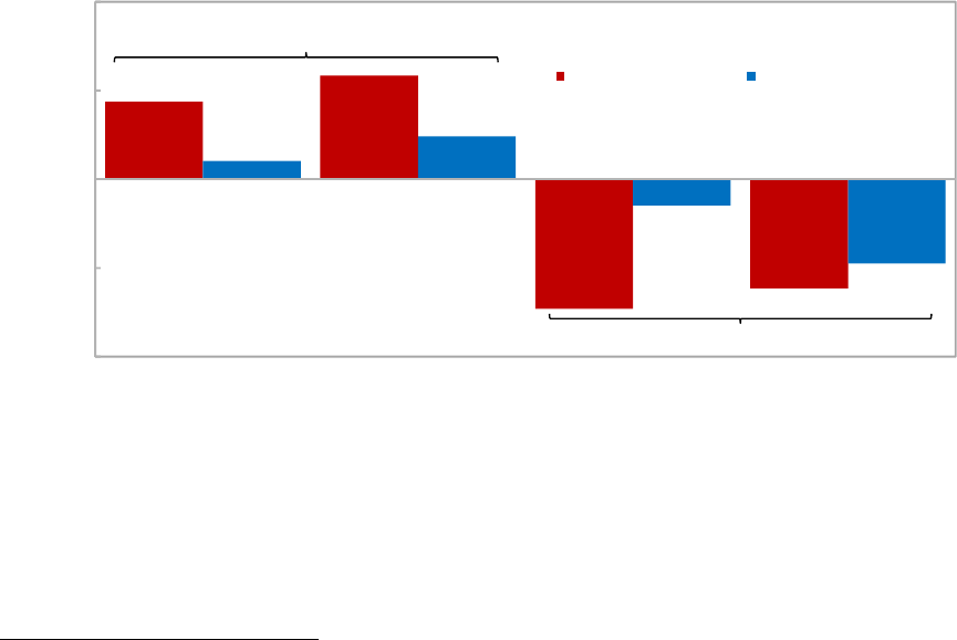
The volatility in commodity prices can have a large impact on the external current and fiscal

accounts. The average direct impact can be estimated based on the average amplitude of

commodity price changes and applying it to fiscal revenues (exports) of resource-rich countries.

As shown in Figure 1, the impact is large, ranging from 8-13 percent of GDP for fiscal revenues

and 2-10 percent of GDP for exports. The relatively larger impact on fiscal revenues in oil

exporters suggests that transmission of commodity price shocks to the economy mostly works

through the fiscal channel. This is in line with results of Husain and others (2008). There is also

evidence of asymmetry across phases of the commodity price cycle, with the impact being

stronger in downswings compared to upswings.

Figure 1. Impact of commodity price swings on fiscal revenues and exports

Source: IMF World Economic Outlook and authors’ estimates.

Note: For upswings (downswings), the impact is estimated by multiplying fiscal revenue and exports as a share of

GDP during the most recent trough (peak) by the average percentage change of commodity prices from trough

to peak (peak to trough). Following Cashin and others (2002), the following parameters are used to date

commodity cycles for the period 1957-2015: minimum duration of each phase = 12 months, minimum duration

of a complete cycle = 24 months.

Table 1 provides descriptive statistics of commodity prices. The analysis is based on commodity prices in USD

by the U.S. GDP deflator.

-20

-10

Fiscal revenue Exports Fiscal revenue Exports

Percent of GDP (average)

Oil exporters Metal exporters

Upswings

Downswings

Past and recent experiences also show that shocks can be very large for the budget and the

economy. Typically, economic activity and external and fiscal balances deteriorate (improve)

during commodity price downswings (upswings).

These price fluctuations can have a significant

impact on growth. For example during the 1970s-80s boom and bust, many countries

experienced revenue increases of close to 10 percent a year in real terms during the boom and

subsequent large falls in the bust (Figure 2). This led to large increases in public expenditures and

economic activity. But, after the bust, many commodity exporters experienced a long period of

negative or stagnant growth. Similarly, many commodity exporters—after experiencing large

revenue windfalls in the 2000s—are now having to manage a large fall in commodity prices.

Many countries will need to endure large fiscal contractions at a time of weak economic activity.

See April 2012 IMF World Economic Outlook.

100

150

200

250

1970 75 80 85 90 95

Saudi Arabia

Algeria

Venezuela

Nig e ria

Norw ay

Iran

With few exceptions, most oil exporters faced a

long period of low growth after commodity prices

fall in the 1980s

(Real GDP per capita, 1970 = 100)

As did most metal exporters

(Real GDP per capita, 1970 = 100)

300

600

900

100

150

200

250

1970 75 80 85 90 95

Chile

Mali

Peru

Botsw ana

(Right hand axis)

Ghana

Zambia

-10

-5

Real revenue

(growth rate)

Real expenditure

(growth rate)

Overall balance

(percent of GDP)

Percent

Before

During

After

Before, During, and After the 1973

‐

80 Boom

Commodity Prices

(U.S. dollars, deflated by U.S. GDP deflator)

Figure 2. The 1970s - 80s boom-bust had a long-lasting negative impact on growth for commodity

exporting countries

Sources: IMF staff estimates.

Note: For panel 2, before = 1971–72, during = 1973–80, after = 1982–83.

100

200

300

400

1970 1975 1980 1985 1990 1995 2000

Oil

Gold

Copper

IV. FISCAL CYCLICALITY

As shown in the literature, by exacerbating output volatility, procyclical fiscal policy could

dampen economic growth. Fatas and Mihov (2003) show that aggressive use of discretionary

fiscal policy adds to economic volatility and lowers economic growth. The Fiscal Monitor (IMF

2015b) finds that an increase in fiscal stabilization (equivalent to one standard deviation of the

sample) would boost long-run annual growth rates of developing economies by 0.1 percentage

points. Van der Ploeg and Poelhekke (2008) also show that volatility hurts growth among

commodity exporters, with the former partially explained by volatile government expenditures.

Resource-rich countries should benefit from countercyclical policies to a greater extent than

other countries. As the large volatility in prices is transmitted to the economy, this could lead to

large swings in the economy. Fiscal policy can help stabilize the economy, especially as the

government usually receives a large share of commodity receipts. However, evidence seems to

suggest that fiscal policy, in many cases, has not been helpful. This is something that Gelb and

associates (1998) already stressed during the 1970s-80s boom and bust. Some argue policies

have become less procyclical (or even countercyclical) in recent years (Frankel and others, 2013;

Céspedes and Velasco, 2014). However, many countries have raised expenditures massively

during the latest revenue windfall and are now being forced to large procyclical expenditure cuts

(IMF 2015a).

Taking advantage of our new dataset for non-renewable resource-rich countries, we revisit the

evidence on fiscal cyclicality and whether it has changed over time, especially during the latest

resource boom. The analysis is based on two alternative approaches: (i) the first measures the

responsiveness of public expenditure growth rates to year-to-year changes in commodity prices;

and (ii) the second looks at the extent to which fiscal policy is reacting to the business cycle in

the non-resource sector.

A. Measure 1: Commodity prices and government spending

The first approach looks at the relation between commodity prices and government

expenditures. A positive association indicates that fiscal policy is procyclical, as government

spending would increase in periods of economic expansion fueled by growing commodity prices

(Arezki, Hamilton, and Kazimov, 2011; Céspedes and Velasco, 2014). The advantage of this

approach is that commodity prices are exogenous to domestic economic cycles and spending

policies, which alleviates endogeneity issues. In addition, as historical experience shows, fiscal

policy tends to react to movements in commodity prices mainly via expenditures. The drawback

is that while commodity price cycles are a key determinant of the domestic economy cycle, they

are not perfectly correlated.

The empirical specification takes the following form:



log

















log













, (1)

in which RG is the real government spending. P is the country-specific commodity price index,

measured as:







∑





∗

∈

, (2)

in which i is the country, j is the commodity type (oil, gas, gold, tin, zinc, lead, aluminum, nickel,

copper, and silver), P is the real commodity price (deflated by the U.S. consumer price index, CPI),

and w is the commodity weight (commodity export share in GDP).

By using changes of government spending and commodity price variables we are abstracting

from the long-run correlation of their levels. In addition, we found no evidence of a long-term

relationship between the two.

Changes of these variables proxy cyclical movements and positive association between changes

is an indication of procyclicality; thereby government spending expands (contracts) domestic

demand in good (bad) times, exacerbating non-commodity business cycles in a procyclical

fashion. We also assess whether there are differences in procyclicality across expansionary and

contractionary phases of the cycle, by interacting commodity price changes with a dummy

variable indicating the cyclical phase.

The results suggest that commodity prices have a positive impact on government spending

(Table 4), implying a procyclical fiscal policy. A 10 percent increase (fall) in commodity prices

leads to a 1.2 percent increase (fall) in real expenditure growth.

This means that, for example, if

oil prices fall by 50 percent, as in the second half of 2014, expenditures would need to contract

by 6.5 percent on average—this at a time when economic growth is rapidly decelerating. The

results are robust when we control for the degree of dependence on resource revenue. When

distinguishing between different stages of the cycle, the results suggest that procyclicality is

stronger during commodity price expansions.

The analysis also indicates that procyclicality has not changed significantly over time. There are

some country examples that suggest they saved more during the latest windfall and were able to

adopt countercyclical fiscal policies in 2009 in response to the international crisis (e.g., Abdid and

others, 2010). However, this was only a very temporary fall in prices and after a massive revenue

windfall—as such, it would be risky to assess fiscal policy only based on that episode. In addition,

Céspedes and Velasco (2014)’s assessment that the fiscal stance was countercyclical in recent

years is problematic as it (in part) relies on using fiscal indicators that are not appropriate for

resource-rich countries, like the overall fiscal balance as a share of total GDP (we address this

The long-term relationship could be positive as countries could afford higher (lower) spending when prices are

higher (lower). However, panel cointegration tests (Westerlund, 2007) suggest the two series are not co-integrated,

which further supports our empirical approach of focusing on changes in expenditures and prices.

Capital spending is even more procyclical compared to total spending (the coefficient is 0.15 and increases to

0.17 when controlling for dependence on resource revenue).

issue below). In fact, we do not find strong evidence that average procyclicality has declined

since 1970. In particular, the regressions based on 10-year rolling windows show that average

procyclicality in recent years is similar to levels seen in past decades (Figure 3). Our result is

consistent with the evidence that many resource-rich countries accelerated significantly public

expenditures during the 2000s, at a time when commodity prices were exceptionally high (or

rising fast). In some countries public expenditures (in real terms) more than tripled during that

period (IMF 2015a).

Figure 3. The degree of procyclicality appears to have been stable over time

B. Measure 2: The cyclically-adjusted non-resource balance

The second approach looks at a more traditional measure of cyclicality. In particular, the

relationship between output gap and cyclically adjusted fiscal balances. If this relationship is

negative, then fiscal policy is procyclical. However, as mentioned above, for resource-rich

countries, a more appropriate indicator of the fiscal stance is the non-resource fiscal balance as a

share of the non-resource GDP instead of the overall balance. This avoids the positive bias when

measuring fiscal cyclicality (Villafuerte and others, 2010).

The empirical specification takes the

following form:

Overall fiscal balances and GDP are heavily influenced by movements in commodity prices and as such should

not be used to assess how policies are changed in response to prices. For example, an improvement in fiscal

-.2 0 .2 .4 .6

1980 1985 1990 1995 2000 2005 2010 2015

Note: Estimations are performed using 10 year rolling windows. Dashed lines represent 10 percent confidence intervals.

(panel regressions)

Time-varying procyclicality of government spending to commodity prices

__



_







_







, (3)

in which CA_BAL_NC is the cyclically adjusted non-resource balance (assuming elasticities of 1 for

revenues and 0 for expenditures), GDP_NC is the non-resource GDP, and GAP_NC is the non-

resource GDP gap. Coefficient  captures the degree of fiscal cyclicality (a negative coefficient

implies procyclicality). The equation is estimated using the fixed effects estimator. In order to

assess robustness of the results, non-resource GDP growth is used instead of the non-resource

output gap, given the high uncertainty when measuring output cycles.

The results suggest that governments tend to loosen the fiscal stance when the domestic non-

resource economy strengthens, and tighten the fiscal stance when the economy weakens

(Table 5), confirming the procyclical bias of fiscal policy. A 1 percentage point improvement in

the non-resource output gap leads to a 1 percentage point deterioration of the cyclically

adjusted non-resource balance as a share of potential non-commodity GDP. Replacing output

gap with real GDP growth rates (for the non-resource economy) does not alter the negative

association. Moreover, commodity exporters tend to be more procyclical than other emerging

economies. Notably, IMF (2015b) found that emerging markets and developing economies also

tend to act procyclically in expansions, but with a coefficient half of the size of the figure found

here for commodity exporters (around 0.5).

C. Can institutions help reduce procyclicality?

Why fiscal policies tend to be procyclical if this leads to volatility and potentially much weaker

growth? Given that commodity price shocks can be very persistent, public expenditures may be

increased significantly if revenues are expected to remain high for long. Once prices disappoint,

there is a need for expenditure cuts. While the decision to respond in a procyclical fashion to

movements in prices may be consistent with affordability arguments (if richer, it could be optimal

to raise spending), it is not so when considering stabilization objectives. As the commodity

windfall is likely to boost the domestic economy, accelerating public spending may be

destabilizing.

Furthermore, countries may expand spending beyond what is feasible under

affordability considerations. For example, Manzano and Rigobon (2001) argue that the problems

faced by resource-rich countries mainly reflect debt overhang as countries borrow during booms

and need to adjust during busts. This, at least in part, reflects the weak political institution

balances when commodity prices rise does not imply there was a tightening of the fiscal stance (the opposite

may be true). Similarly, governments may react to a rise in prices by boosting expenditures and lead to a strong

fiscal impulse to the domestic economy, even when the overall fiscal balance improves—thanks to a large

increase in commodity revenue (originated from export receipts).

The large scaling up of public spending could also have a negative impact on its quality and effectiveness. See

IMF (2015a) for more discussion on this.

argument which identifies these economies as more prone to rent-seeking in the face of large

commodity windfalls (Tornell and Lane, 1999).

In an attempt to restrict fiscal policy, many countries have adopted fiscal rules and resource

funds, more generally defined as special fiscal institutions. Special fiscal institutions collect a

large number of rules, mechanisms and devices specifically aimed at the management of

commodity revenues from a fiscal perspective.

In this section we look at the impact of these

rules and resource funds on procyclicality.

For our analysis, we consider only rules that have been strictly designed to regulate the

accumulation or use of resource revenues, including rules that are established for the functioning

of a fund (either saving or stabilization fund). At times funds have been established without a

legally binding rule for the accumulation and withdrawal of assets. Hence, the estimation below

features both a dummy for fiscal rules and a dummy for when a fund is in place (with or without

a rule). To complement the analysis, we will also look at the impact of broader political

institutions. We selected some institutional variables from the World Governance Indicators and

the International Risk Group databases; notably bureaucratic quality, corruption, political risk and

strength of the institutional and legal setting. The Polity variable comes from the Polity IV dataset

and captures the quality of democratic institutions and rule of law.

To analyze the impact of institutional characteristics and fiscal rules and resource funds, the

commodity price index is interacted with respective measures of institutional quality and fiscal

rules/resource funds. The empirical specification takes the following form:

 log













 log









 log









∗







, (4)

in which I stands for the index of institutional quality (a continuous variable) and the existence of

a fiscal rule or a resource fund in place (a dummy variable). Coefficient



measures the extent to

which institutions and rules/funds can affect procyclicality (a negative coefficient would imply a

reduction in procyclicality in countries with better institutions and fiscal rules/resource funds).

The estimation results suggest that experience with resource funds and fiscal rules has been

mixed (Table 6). While the interaction term is negative, consistent with the hypothesis of a

reduction in procyclicality following the adoption of fiscal rules/resource funds, it is not

significant. The econometric findings match with the widespread empirical evidence where with

the exception of notable successes in Botswana, Chile, and Norway, many other countries are still

These fiscal rules are different from the more common rules aimed at restricting fiscal policy at large and

adopted also by countries other than resource rich (for a description of the latter see Schaechter and others,

2012, and the IMF database http://www.imf.org/external/datamapper/FiscalRules/map/map.htm). Other types of

special fiscal institutions include stabilization funds, saving funds, and investment funds when the latter are

related to the investment of resource receipts (see Table 9 in the appendix with the rules and institutions

considered in this paper).

struggling to improve compliance and efficacy of their special fiscal institutions. Reasons for this

lack of success are varied.

The existence of a fiscal rule or fiscal fund does not necessarily indicate a de facto compliance

with the rule. As evidence shows many rules tend to be breached especially in bad times. Lack of

compliance could be due to several factors, such as lack of political will, poor design of the rule

and absence of monitoring and enforcement bodies. In Nigeria, for example, the rule was

repeatedly undermined by weak enforcement. In other countries, like Chad, Ecuador, and Timor

Leste, rules were breached as they became incompatible with budget and developmental

priorities of the authorities. In some other cases, due to the rule design, governments embarked

in extra-budgetary operations which made the rules ineffective and weakened budgetary control

(Mongolia, Azerbaijan, Kazakhstan and Libya). In some cases, lack of coordination between the

activities related to a resource fund and ordinary budgetary operations resulted in accumulation

of financial assets in funds at times when governments had to borrow expensively to finance

deficits (Ghana and Trinidad and Tobago).

There is empirical support, however, that the quality of political institutions helps limit the

procyclical bias in spending.

In some cases the impact can be highly significant (Table 7). For

example, procyclicality would be eliminated in countries with the degree of bureaucratic quality

or quality of institutional and legal setting around two standard deviations above the mean. In

part, this reflects the fact that the average quality of institutions tends to be weaker in resource-

rich countries than in other countries (Figure 4). This evidence also suggests that the lack of

success of rules and funds in some countries may owe more to the underlying weaknesses of

their institutional frameworks than to the rules themselves.

Some countries have been successful in limiting the negative impact of the commodity prices

volatility and promote sustainable economic growth. Namely, the quality of institutions in

Norway, Chile, and Botswana is higher than among their peers, which helped support fiscal policy

and achieve stronger and higher long-term growth (see Figure 2). They also show that fiscal rules

or resource funds can help achieve policy objectives if they are supported by strong institutions

and political commitment, are well-designed, and are closely linked to broader policy objectives.

The examples of Chile and Norway show that the rules can both help discipline policies and allow

See Ossowski and others (2008) and Sugawara (2014) for a review.

These results are similar to those found in earlier studies (Ossowski and others, 2008). Frankel and others

(2013) also stress the importance of quality of institutions, while Akitoby and others (2004) argue strengthening

checks and balances can also help reduce the cyclicality of government expenditures.

for flexibility to respond to economic conditions—thanks to large financial buffers built during

resource booms and strong market credibility.

13, 14

Figure 4. Institutional quality in resource-rich countries is weaker than in other countries

Source: Worldwide Governance Indicators (World Bank) and authors’ estimates.

Note: The chart shows average levels of institutional quality for resource-rich and resource-poor countries with

the same level of GDP per capita (sample average for resource-rich countries). Larger numbers indicate higher

institutional quality. Sample period: 1996-2014.

The strong institutional framework allowed Chile to react in a countercyclical fashion to the sudden and large

2008-09 commodity price fall. During the commodity boom, Chile increased net financial assets significantly. This

allowed a large easing of fiscal policy in 2008-09 in response to the global financial crisis (went from a 8 percent

overall surplus in 2007 to a 4 percent fiscal deficit in 2009). See also Frankel (2011) for further discussion on Chile.

The Norwegian fiscal framework is anchored on a strong political commitment to a non-oil balance target.

Oil/gas revenue is saved in an oil fund and only the returns from financial investments are used to fund the

budget. Under the framework, the non-oil deficit should average 4 percent of the assets in the oil fund over the

economic cycle. The rule allows to insulate the budget from yearly movements in the oil and gas prices. Norway’s

framework has not only resulted in the buildup of large financial savings, but also helped sustain GDP per capita

growth above most other resource-rich countries over the last 4 decades.

-0.5

-0.4

-0.3

-0.2

-0.1

0.0

0.1

0.2

Voice and Accountability

Political Stability

Government

Effectiveness

Regulatory Quality

Rule of Law

Control of Corruption

Resource-poor Resource-rich

V. HOW DO NON-RESOURCE REVENUES RESPOND TO COMMODITY REVENUE SHOCKS?

In this section we analyze how non-resource revenues react to fluctuations in commodity

revenues (heavily influenced by commodity prices). Most of previous studies on how resource-

rich countries react to commodity price shocks has focused on expenditures—as, indeed, it tends

to be the main channel. However, countries can also respond to shocks by changing their tax

effort.

The existing studies assess the reaction of non-resource revenues to persistent changes in

commodity revenues in oil/gas exporters (see Bornhorst and others, 2009; Thomas and Trevino,

2013; Crivelli and Gupta, 2014). They find that countries tend to offset rising commodity revenue

by a reduction in non-resource tax effort.

We expand the analysis in two main directions: (i) we use a broader set of commodity exporters

and scale the commodity and non-commodity revenues by the non-commodity GDP to alleviate

the endogenous impact of commodity price changes on the denominator, and (ii) we analyze

both long-run and short-run reaction to changes in commodity revenues using the Pooled Mean

Group (PMG) estimator of Pesaran and others (1999). The empirical specification is:

 



























 















 



















, (5)

in which i and t indexes denote country and time, Y is the nominal GDP (non-commodity), R is

government non-commodity (NC) and commodity (C) revenues, µ is the country-specific fixed

effect, and



is an i.i.d. error term. The term in the squared bracket is the error-correction term

measuring the extent of the deviation of the non-commodity revenue from its long-run

equilibrium value.



measures the long-run reaction of non-commodity revenues to a permanent

change in commodity revenues and corresponds to the coefficient estimates in Bornhorst and

others (2009), and Crivelli and Gupta (2014). Similarly,



measures the short-term effect of non-

commodity revenue to a temporary change in non-commodity revenue.  is the speed of

adjustment of non-commodity revenue to its long-run equilibrium: the larger is the coefficient (in

absolute terms), the faster is the adjustment. Finally, the country-specific fixed effects included in

the specification capture unobserved heterogeneity of non-commodity revenue across different

countries.

Our results suggest that resource-rich countries adjust tax effort in response to persistent

changes in commodity revenues, but there is limited reaction to temporary changes. Table 8

shows that a permanent increase in commodity revenues by 1 percent of non-commodity GDP

tends to reduce non-commodity revenues by 0.03-0.04 percent of non-commodity GDP.

Temporary changes in commodity revenues (up to three years lag) do not have a significant

A 1 percent of GDP increase in hydrocarbon revenues leads to about 0.2 percent reduction of non-

hydrocarbon revenues over the long-run (Bornhorst and others, 2009).

impact on non-commodity revenues. Countries do not seem to change non-commodity revenue

effort in response to temporary commodity revenue shocks, letting the automatic stabilizers

work. In addition, half of the deviation from the long run association between commodity and

non-commodity revenues is corrected in four years, providing further evidence on the sluggish

adjustment of non-commodity revenues.

VI. C

ONCLUSIONS

Fiscal policy in resource-rich countries tends to be highly procyclical and more so than for other

economies. Contrary to other studies, we do not find evidence that procyclicality has declined

over time. We also find that adoption of fiscal rules or resource funds do not have a significant

impact on fiscal cyclicality, but general political institutions do help. The lack of progress on these

likely partly explains why fiscal procyclicality, on average, has not declined in recent years.

Our results have important policy implications. First, more efforts are needed to establish a

comprehensive fiscal policy framework in resource-rich countries that can help cope with

heightened uncertainty and volatility. These frameworks should be based on a solid long-term

anchor to guide fiscal policy and should explicitly incorporate commodity price uncertainty. This

means putting more emphasis on building precautionary savings during good times to help

weather shocks in a countercyclical fashion. Next, further efforts to improve the institutional

framework are needed, including enhancing transparency and accountability. Tax policies aimed

at diversifying the revenue base would reduce government’s overdependence on commodity

revenues and improve its ability to run countercyclical policies. Finally, efforts to diversify the

economy beyond the commodity sector are also critical.

ANNEX 1. DATA

The primary data sources for the analysis are the IMF’s International Financial Statistics (IFS),

Balance of Payments Statistics, Direction of Trade Statistics, World Economic Outlook database,

and fiscal rules databases; the World Bank’s World Development Indicators and World Governance

Indicators; the Macro Data Guide Political Constraint Index Dataset (POLCON); POLITY IV and

International Country Risk Guide data. Data for all variables of interest are collected on an annual

basis from 1970 to 2013, where available. We also use monthly data on commodity prices over

1957-2015 period.

The sample is comprised of 48 countries that are exporters of oil, gas, and metals (such as

copper, gold, iron, and silver), where these commodities represent a large share of exports (20

percent or more of total exports) or fiscal revenues (15 percent or more) over a large part of the

period under consideration. The countries are: Algeria, Angola, Australia, Azerbaijan, Bahrain,

Bolivia, Botswana, Brunei Darussalam, Cameroon, Canada, Chad, Chile, Colombia, Democratic

Republic of Congo, Republic of Congo, Côte d'Ivoire, Ecuador, Gabon, Ghana, Guinea, Guyana,

Indonesia, Iran, Iraq, Kazakhstan, Kuwait, Libya, Mali, Mauritania, Mexico, Mongolia, Nigeria,

Norway, Oman, Papua New Guinea, Peru, Qatar, Russia, Saudi Arabia, South Africa, Sudan,

Suriname, Syria, Trinidad and Tobago, United Arab Emirates, Venezuela, Yemen, and Zambia. The

sample varies for each analysis depending on data availability.

Tables

Table 1. Descriptive statistics: Commodity price growth rates

Source: IMF World Economic Outlook.

Note: Reported are descriptive statistics for real m-o-m growth rates.

Sample Obs. Mean Median St. Dev. Skewness Kurtosis

Aluminium Feb 1957-Jan 2015 696 -0.133 -0.188 4.66 -0.504 8.380

Copper Feb 1957-Jan 2015 696 -0.009 0.084 6.63 -0.477 6.351

Gold Feb 1957-Jan 2015 612 0.254 -0.199 4.69 1.091 11.563

Iron ore Feb 1975-Jan 2015 480 0.145 -0.295 5.56 3.812 36.452

Gas (EU) Feb 1985-Jan 2015 360 0.033 -0.206 6.43 -0.635 18.460

Gas (US) Feb 1991-Jan 2015 288 0.063 -0.310 13.34 -0.042 3.950

Tin Feb 1957-Jan 2015 696 0.008 -0.107 4.98 -0.474 6.719

Oil (Brent) Feb 1957-Jan 2015 696 0.146 -0.243 8.38 4.354 65.932

Oil (Texas) Feb 1957-Jan 2015 696 0.099 -0.279 7.11 2.088 34.853

Table 2. Duration of commodity price expansions and contractions

Source: IMF World Economic Outlook and authors’ calculations.

Note: Phases of expansions and contractions are defined using the Harding and Pagan (2002)

algorithm. Sample period: January 1957-March 2015.

Mean Median St. Dev. Freq. Min Max

Expansions 29.3 18.0 24.4 11 11 86

Contractions 34.1 34.0 14.6 11 12 65

Expansions 38.5 24.5 33.0 8 17 112

Contractions 43.2 44.0 26.9 9 12 81

Expansions 36.4 26.0 38.7 8 3 125

Contractions 40.3 33.5 22.1 8 17 79

Expansions 29.2 13.0 34.6 6 12 99

Contractions 43.7 47.0 20.9 7 11 72

Expansions 30.8 24.5 23.9 6 7 76

Contractions 29.3 27.0 13.6 6 15 53

Expansions 23.8 19.0 15.9 6 13 55

Contractions 20.9 15.0 14.5 7 6 47

Expansions 25.1 23.0 8.8 11 12 38

Contractions 35.1 19.0 46.5 12 14 179

Expansions 28.3 21.0 20.5 11 12 79

Contractions 32.2 23.5 30.3 12 8 107

Expansions 28.3 22.5 21.3 10 12 78

Contractions 37.6 23.0 35.1 11 8 115

Oil-Texas

Tin

Oil-Brent

Gas-EU

Gas-US

Gold

Iron ore

Alluminium

Copper

Table 3. Amplitude of commodity price expansions and contractions

Source: IMF World Economic Outlook and authors’ calculations.

Note: Phases of expansions and contractions are defined using the Harding and Pagan (2002) algorithm.

Sample period: January 1957-March 2015.

Mean Median St. Dev. Freq. Min Max

Expansions 40.9 52.4 35.0 11.0 1.6 107.1

Contractions -51.6 -49.6 42.2 11.0 -140.0 -6.2

Expansions 78.6 70.2 45.6 8.0 25.2 172.0

Contractions -72.4 -85.4 34.5 9.0 -113.1 -17.1

Expansions 63.3 28.9 64.3 8.0 7.3 166.1

Contractions -47.5 -48.5 24.4 8.0 -91.1 -9.9

Expansions 50.4 14.4 96.0 6.0 0.9 245.6

Contractions -35.9 -27.3 35.5 7.0 -107.6 -5.9

Expansions 63.6 54.2 58.7 6.0 3.0 168.8

Contractions -63.4 -58.7 30.5 6.0 -113.0 -21.5

Expansions 80.1 84.3 25.1 6.0 33.7 110.5

Contractions -78.9 -69.5 49.3 7.0 -154.9 -14.4

Expansions 50.6 49.3 34.2 11.0 9.0 117.1

Contractions -47.8 -44.6 48.2 12.0 -192.2 -12.3

Expansions 63.0 57.3 51.5 11.0 4.2 175.4

Contractions -57.8 -51.2 43.6 12.0 -162.7 -2.9

Expansions 65.5 63.0 50.6 10.0 0.4 166.7

Contractions -51.8 -45.7 40.1 11.0 -138.6 -9.3

Oil-Texas

Tin

Oil-Brent

Iron ore

Gas-EU

Gas-US

Alluminium

Copper

Gold

Table 4. Estimation results: Government spending and commodity prices

Note: Dependent variables are real total expenditure (Columns I-IV), and capital expenditure (Columns V-VIII) growth

rates. Estimations are performed using the fixed effects estimator with AR(1) residuals and time effects. Robust

standard errors are in brackets. *, **, and *** denote significance at 10, 5, and 1 percent levels, respectively.

Table 5. Estimation results: Non-commodity output gap and cyclically-adjusted non-

commodity balance

Note: Dependent variable is cyclically-adjusted non-commodity balance. Estimations are performed using the

fixed effects estimator with time effects. Robust standard errors are in brackets. *, **, and *** denote significance

at 10, 5, and 1 percent levels, respectively.

III

Non-commodity output gap -0.945***

[0.225]

Non-commodity GDP growth -0.215***

[0.011]

Constant -0.266*** -0.254***

[0.039] [0.039]

Observations 770 765

Number of countries 41 41

R^2 0.14 0.279

I II III IV V VI VII VIII



log of commodity prices

0.119** 0.121** 0.147* 0.169**

[0.052] [0.057] [0.081] [0.086]



log of commodity prices*Dummy (=1 for commodity price expansions)

0.148** 0.157** 0.205** 0.223**

[0.059] [0.065] [0.095] [0.101]



log of commodity prices*Dummy (=1 for commodity price contractions)

0.073 0.070 0.074 0.102

[0.068] [0.072] [0.103] [0.108]

Share of commodity sector value added in GDP 0.004*** 0.004*** 0.006*** 0.006***

[0.001] [0.001] [0.001] [0.001]

Constant 0.124** 0.038 -1.193 -1.198 0.055 0.017 0.029 0.034

[0.058] [0.045] [1.281] [1.245] [0.058] [0.054] [1.145] [1.153]

Observations 902 902 824 824 1346 1346 1239 1239

Number of countries 4141414138383838

R^2 0.079 0.080 0.107 0.109 0.079 0.080 0.102 0.103

Dependent variable: total expenditure growth

rate

Dependent variable: capital expenditure

growth rate

Table 6. Impact of fiscal rules on fiscal procyclicality

Note: Dependent variable is real expenditure growth rate. Estimations are performed using the fixed effects

estimator with AR(1) residuals and time effects. Robust standard errors are in brackets. *, **, and *** denote

significance at 10, 5, and 1 percent levels, respectively.

Table 7. Impact of institutions on fiscal procyclicality

Note: Dependent variable is real expenditure growth rate. Estimations are performed using the fixed effects

estimator with AR(1) residuals and time effects. Robust standard errors are in brackets. *, **, and *** denote

significance at 10, 5, and 1 percent levels, respectively.

I II III IV V



log of commodity prices

0.119** 0.143** 0.164** 0.151** 0.176**

[0.052] [0.066] [0.069] [0.063] [0.070]



log of commodity prices*Savings fund dummy

-0.022

[0.071]



log of commodity prices*Stabilization fund dummy

-0.058

[0.064]



log of commodity prices*Fiscal rule dummy

-0.078

[0.088]



log of commodity prices*Fiscal rule or savings/stabilization fund dummy

-0.075

[0.063]

Constant 0.124** 0.123* 0.125* 0.125* 0.128*

[0.058] [0.073] [0.073] [0.073] [0.073]

Observations 902 718 718 718 718

Number of countries 4134343434

R^2 0.079 0.083 0.084 0.084 0.085

I II III IV V VI



log of commodity prices

0.119** 0.142* 0.341*** 0.214** 0.609*** 0.266**

[0.052] [0.076] [0.090] [0.095] [0.178] [0.115]



log of commodity prices*Polity

-0.008

[0.006]



log of commodity prices*Bureaucratic quality

-0.087***

[0.029]



log of commodity prices*Corruption

-0.027

[0.024]



log of commodity prices*Political risk

-0.007***

[0.002]



log of commodity prices*Institutional and legal setting

-0.003*

[0.001]

Constant 0.124** 0.155* 0.05 0.039 0.034 0.127**

[0.058] [0.086] [0.055] [0.056] [0.028] [0.060]

Observations 902 464 805 805 804 716

Number of countries 412241414133

R^2 0.079 0.101 0.089 0.079 0.088 0.092

Table 8. Impact of commodity revenue shocks on non-commodity revenues

Note: Dependent variable is the change in non-commodity revenue ratio. Estimations are performed using the

Pooled Mean Group (PMG) estimator. *, **, and *** denote significance at 10, 5, and 1 percent levels, respectively.

I II III

Long-run coefficients

Commodity revenue/non-commodity GDP (lagged) -0.033*** -0.035*** -0.040***

[0.007] [0.008] [0.007]

Constant 19.576*** 19.829*** 20.006***

[0.412] [0.463] [0.380]

Short-run coefficients

Speed of adjustment -0.156*** -0.150*** -0.169***

[0.042] [0.044] [0.045]

 Commodity revenue/non-commodity GDP

-0.072 -0.046 -0.085

[0.075] [0.102] [0.150]

 Commodity revenue/non-commodity GDP (1 lag)

-0.057 -0.071

[0.132] [0.207]

 Commodity revenue/non-commodity GDP (2 lags)

-0.244

[0.175]

Observations 744 703 676

Log likelihood -1545.3 -1432.0 -1321.0

Half life (years) 4.1 4.3 3.7

Table 9. Resource funds and rules

Note: 1/ Sovereign Wealth Funds (SWF) here capture only saving and stabilization funds.

SWF 1/

Yes=1; No=0 Yes=1; No=0 Dates Yes=1; No=0 Dates Yes=1; No=0 Dates

Algeria 1 0 1 2000 0

Angola 1 1 2012 1 2012 0

Azerbaijan 1 1 1999 1 1999 1 1999

Bahrain 1 0 1 2000 0

Bolivia 0 0 0 0

Botswana 1 1 1993 1 1972 1 1994

Brunei Darussalam 0 0 0 0

Cameroon 0 0 0 0

Chad 1 1 2008 1 2008 0

Chile 1 1 1985 1 1985 1 2006

Colombia 1 0 1 1995 0

Congo 0 0 0 0

Congo DRC 0 0 0 0

Cote D'Ivoire 0 0 0 0

Equatorial Guinea 1 1 2002 0 1 2002

Ecuador 1 1 2005 1 1999-2007 1 2002

Gabon 1 1 1998 0 1 1998

Ghana 1 1 2011 1 2011 1 2011

Guinea 0 0 0 0

Guyana 0 0 0 0

Indonesia 0 0 0 0

Iran 1 0 1 2000 0

Iraq 0 0 0 0

Kazakhstan 1 1 2000 1 2000 1 2000

Kuwait 1 1 1960 1 1960 0

Libya 1 1 1995 0 0

Mali 0 0 0 0

Mauritania 1 0 1 2000 0

Mexico 1 0 1 2000 0

Mongolia 1 0 1 2011 0

Mozambique 0 0 0 0

Niger 0 0 0 0

Nigeria 1 1 2011 1 2004 0

Norway 1 1 1985 1 1985 1 2002

Oman 1 1 1980 0 0

Papua New Guinea 1 0 1 1974-2001 0

Peru 1 0 1 1999 0

Qatar 1 0 1 2000 0

Russia 1 0 1 2004 1 2008

Saudi Arabia 0 0 0 0

Sudan 1 0 1 2002 0

Suriname 0 0 0 0

Syria 0 0 0 0

Timor Leste 1 1 2005 1 2005 1 2005

Trinidad and Tobago 1 1 1999 1 2005 1 2007

UAE 0 0 0 0

Venezuela 1 1 1999 0 1 2000

Yemen 0 0 0 0

Zambia 0 0 0 0

Saving Fund Stabilization Fund Fiscal Rule

REFERENCES

Abdih, Y., Lopez-Murphy, P., Roitman, A., and Sahay, R., 2010, "The Cyclicality of Fiscal Policy

in the Middle East and Central Asia: Is the Current Crisis Different?" IMF Working

Paper 10/68 (Washington: International Monetary Fund).

Akitoby, B., B. Clements, S. Gupta, and G. Inchauste, 2004, “The Cyclical and Long-Term

Behavior of Government Expenditures in Developing Countries,” IMF Working Paper

04/202 (Washington: International Monetary Fund).

Akitoby, B., B. Clements, S. Gupta, and G. Inchauste, 2006, “Public Spending, Voracity, and

Wagner’s Law in Developing Countries,” European Journal of Political Economy, 22:

908-24.

Alesina, A., F. Campante, and G. Tabellini, 2008, “Why is Fiscal Policy Often Procyclical?”

Journal of the European Economic Association, 5 (5): 1006–36.

Arezki, R., K. Hamilton, and K. Kazimov, 2011, “Resource Windfalls, Macroeconomic Stability

and Growth: The Role of Political Institutions,” IMF Working Paper 11/142,

(Washington: International Monetary Fund).

Bornhorst, F., S. Gupta, and J. Thornton, 2009, “Natural Resource Endowments and the

Domestic Revenue Effort,” European Journal of Political Economy 25: 439–46.

Cashin, P., J. McDermott, and A. Scott, 2002, “Booms and Slumps in World Commodity

Prices,” Journal of Development Economics, 69 (1): 277–96.

Céspedes, L., and A. Velasco, 2014, “Was This Time Different? Fiscal Policy in Commodity

Republics,” Journal of Development Economics, 106: 92–106.

Crivelli, E., and S. Gupta, 2014, “Resource Blessing, Revenue Curse? Domestic Revenue Effort

in Resource-Rich Countries,” European Journal of Political Economy, 35: 88–101.

Erbil, N., 2011, “Is Fiscal Policy Procyclical in Developing Oil-Producing Countries?” IMF

Working Paper 11/171 (Washington: International Monetary Fund).

International Monetary Fund (IMF), 2015a, October Fiscal Monitor, “The Commodities

Rollercoaster: A Fiscal Framework for Uncertain Times,” (Washington).

———2015b, April Fiscal Monitor, “Now is the Time: Fiscal Policies for Sustainable Growth,”

(Washington).

Fatas, A., and I. Mihov, 2003, “The Case for Restricting Fiscal Policy Discretion,” Quarterly

Journal of Economics, 118 (4): 1419–47.

Frankel, J., Vegh, C., and G. Vulletin, 2013, "On Graduation from Fiscal Procyclicality," Journal

of Development Economics, 100: 32-47.

Frankel, J., 2011, "A Solution to Fiscal Procyclicality: The Structural Budget Institutions

Pioneered by Chile,” NBER Working Paper No. 16945 (Cambridge, Massachusetts).

Gali, J. and R. Perotti, 2003, "Fiscal Policy and Monetary Integration in Europe," Economic

Policy, 18(37): 533-572.

Gavin, M., and R. Perotti, 1997, “Fiscal Policy in Latin America,” In NBER Macroeconomics

Annual, edited by Ben S. Bernanke and Julio J. Rotemberg, (Cambridge,

Massachusetts: MIT Press).

Gelb, A., and Associates, 1998, Oil Windfalls: Blessing or Curse? (Oxford University Press).

Ghosh, Atish R., Jun I. Kim, and Mahvash S. Qureshi, 2010, “Fiscal Space,” IMF Staff Position

Note 10/11 (Washington: International Monetary Fund).

Gourinchas, Pierre-Olivier, and Maurice Obstfeld, 2011, “Stories of the Twentieth Century for

the Twenty-First,” NBER Working Paper No. 17252 (Cambridge, Massachusetts).

Harding, D., and A. Pagan, 2002, “Dissecting the Cycle: A Methodological Investigation,”

Journal of Monetary Economics, 49, 365– 381.

Husain, A., K. Tazhibayeva, and A. Ter-Martirosyan, 2008, “Fiscal Policy and Economic Cycles

in Oil-Exporting Economies,” IMF Working Paper 08/253 (Washington: International

Monetary Fund).

Kaminsky, G., C. Reinhart, and C. Vegh, 2005, "When It Rains, It Pours: Procyclical Capital

Flows and Macroeconomic Policies," NBER Macroeconomics Annual 2004, Vol. 19,

pages 11-82.

Manzano, O., and R. Rigobon, 2001, “Resource Curse or Debt Overhang,” NBER Working

Paper No. 8390 (Cambridge, Massachusetts).

Ossowski, R., M. Villafuerte, P. Medas, and T. Thomas, 2008, “The Role of Fiscal Institutions in

Managing the Oil Revenue Boom,” IMF Occasional Paper 260 (Washington:

International Monetary Fund).

Pesaran, H., Y. Shin, and R. Smith, 1999, “Pooled Mean Group Estimation of Dynamic

Heterogeneous Panels,” Journal of the American Statistical Association, 94 (446): 621–34.

Schaechter, A., T. Kinda, N. Budina, and A. Weber, 2012, “Fiscal Rules in Response to the

Crisis—Toward the “Next-Generation” Rules. A New Dataset,” IMF Working Paper

12/187 (Washington: International Monetary Fund).

Sugawara, N., 2014, “From Volatility to Stability in Expenditure: Stabilization Funds in

Resource-Rich Countries,” IMF Working Paper 14/43 (Washington: International

Monetary Fund).

Thomas, A., and J. Treviño, 2013, “Resource Dependence and Fiscal Effort in Sub-Saharan

Africa,” IMF Working Paper 13/188 (Washington: International Monetary Fund).

Van Der Ploeg, F. and S. Poelhekke, 2008, “Volatility and the Natural Resource Curse,”

OxCarre Research Paper 3, Centre for the Analysis of Resource-Rich Economies,

Oxford University.

Villafuerte, M., P. Lopez-Murphy, and R. Ossowski, 2010, “Riding the Roller Coaster: Fiscal

Policies of Nonrenewable Resource Exporters in Latin America and the Caribbean,”

IMF Working Paper 10/251 (Washington: International Monetary Fund).

Westerlund, J., 2007, “Testing for Error Correction in Panel Data,” Oxford Bulletin of

Economics and Statistics 69: 709–748.

World Bank, 2009, “Global Economic Prospects,” (Washington: World Bank).