Population Density of Northern Spotted Owls in Managed Young-growth Forests in Coastal Northern California

Journal of Raptor Research Journal of Raptor Research

Volume 33 Issue 4 Article 1

January 2024

Population Density of Northern Spotted Owls in Managed Young-Population Density of Northern Spotted Owls in Managed Young-

growth Forests in Coastal Northern California growth Forests in Coastal Northern California

Lowell V. Diller

Darrin M. Thome

Follow this and additional works at: https://digitalcommons.usf.edu/jrr

Recommended Citation Recommended Citation

Diller, Lowell V. and Thome, Darrin M. (2024) "Population Density of Northern Spotted Owls in Managed

Young-growth Forests in Coastal Northern California,"

Journal of Raptor Research

: Vol. 33 : Iss. 4 , Article

Available at: https://digitalcommons.usf.edu/jrr/vol33/iss4/1

This Scienti9c Paper is brought to you for free and open access by the Searchable Ornithological Research Archive

at Digital Commons @ University of South Florida. It has been accepted for inclusion in Journal of Raptor Research

by an authorized editor of Digital Commons @ University of South Florida. For more information, please contact

[email protected].

THE JOURNAL OF RAPTOR RESEARCH

A QUARTERLY PUBLICATION OF THE RAPTOR RESEARCH FOUNDATION, INC.

VOL. 33 DECEMBER 1999 NO. 4

j Raptor Res. 33(4):275-286

¸ 1999 The Raptor Research Foundation, Inc.

POPULATION DENSITY OF NORTHERN SPOTTED OWLS IN

MANAGED YOUNG-GROWTH FORESTS IN COASTAL

NORTHERN CALIFORNIA

LO•T•LL V. DILLER

Simpson Timber Company, P.O. Box 68, Korbel, CA 95550 U.&A.

DARRIN M. THOME

U.S. Fish and Wildlife Service, 2321 West Royal Palm Road, Suite 103, Phoenix, AZ 85021 U.S.A.

ABSTRACT.--We estimated population densities of Northern Spotted Owls (Strix occidentalis caurina) in

managed young-growth forests in coastal northern California from 1991-97. The 1266 km 2 study area

was divided into three subregions (Klamath--666 km 2, Korbel--392 km • and Mad River--208 km 2) and

completely surveyed each of the seven years. A total of 446 individual owls was marked to generate both

empirical and Jolly-Seber (J-S) estimates of density. Mean empirical and J-S estimates of abundance were

similar but mean estimates of crude density (territorial owls/km 2) differed among the three subregions

(Klamath--0.092 _+ 0.006 [_SE], Korbel--0.351 _+ 0.011, Mad River--0.313 _+ 0.017 and overall mean-

0.209 + 0.009). Significant differences in forest age-class composition among the three subregions

provided a plausible explanation for the low Klamath density but did not account for the similar den-

sities observed in -Korbel and Mad River. Ecological densities (number of individuals/area of habitat)

were higher than crude densities but the interpretation of this was limited because only nesting habitat

was used to estimate suitable habitat. Compared to limited published reports, densities were relatively

high in two of the three subregions in our study but this was probably typical of Northern Spotted Owl

densities for portions of coastal northern California. Recognizing the limitations of using density to

indicate habitat quality, our study provided valuable baseline data for assessing long-term trends in

Northern Spotted Owl population dynamics within the study area.

KEY WOP, DS: Northern Spotted Owl; Strix occidentalis caurina; California; density; managed forests; mark-

recapture.

Densidad poblacional de Strix Occidentalis caurina en los bosques jtvenes y manejados de las costas del

norte de California

RESUMEN.--Estimamos la densidad poblacional de Strix occidentalis caurina en bosques jtvenes y mane-

jados de las costas del norte de California entre 1991-97. Los 1266 km a del area de estudio fueron

divididos en tres subregiones (Klamath--666 km a, Korbel--392 km a y Mad River--208 km a) y los mon-

itoreamos durante los siete aftos. Un total de 446 individuos de buhos fueron marcados con el fin de

generar estimativos de densidad empiricos y de Jolly-Seber (J-S). La media empirica y los estimativos

de J-S de abundancia fueron similares, pero la media de densidad cruda (buhos territoriales/km a)

difiri6 en las tres subregiones (Klamath--0.092 + 0.006 [_SE], Korbel--0.351 _ 0.011, Mad River--

0.313 - 0.017 y la media promedio--0.209 + 0.009). Las diferencias significativas en la edad y clase de

la composicitn de los bosques entre las tres subregiones pueden ser la explicacitn de la baja densidad

de Klamath pero no para las densidades similares observadas en Korbel y Mad River. Las densidades

ecoltgicas (nfmero de individuos/area de habitat) fueron mayores que las densidades crudas. La in-

terpretacitn de esta fue limitada debido a que se utiliza el habitat de anidacitn para estimar habitats

convenientes. A1 comparar la limitada publicacitn de reportes, se encontr6 que las densidades fueron

275

276 DILLER AND THOME VOL. 33, NO. 4

relativamente altas en dos de las tres subregiones de nuestro estudio. Quizas esto sea tipico de las

densidades de Strix occidentalis caurina en porciones costeras del norte de California. AI reconocer las

limitaciones de usar densidades para indicar la calidad de habitat, nuestro estudio provee valiosos datos

para evaluar tendencias en el largo plazo sobre la din/unica poblacional de Strix occidentalis caurina

dentro del/trea de estudio.

[Traducci6n de Cfisar M/trquez]

The Northern Spotted Owl (Strix occidentalis

caurina) is associated with mature and old-growth

forests throughout much of its range. This rela-

tionship has been studied primarily through radio-

telemetry data that infers habitat selection through

disproportionate use of mature- and old-growth

forests relative to their occurrence within a land-

scape (Forsman et al. 1984, Carey et al. 1990, Solis

and Guti(•rrez 1990, Carey et al. 1992). In addition,

studies of Northern Spotted Owl occurrence and

abundance have shown a greater number of owl

sites in mature- and old-growth forests relative to

adjacent young forests (Forsman et al. 1977, Fors-

man et al. 1987, Forsman 1988, Bart and Forsman

1992, Blakesley et al. 1992). Given the economic

value of mature- and old-growth forests, the asso-

ciation of Northern Spotted Owls with these forests

places it at the center of a major controversy in the

Pacific Northwest. The 1990 listing of the Northern

Spotted Owl under the federal Endangered Spe-

cies Act (USDI 1992) instituted management pol-

icies limiting timber harvest of Northern Spotted

Owl habitat on public and private lands (Thomas

et al. 1990, Guti(•rrez et al. 1996, Marcot and

Thomas 1997).

The population density of a species is important

to resource managers for several reasons. In har-

vested game species, it is important to increase

population density to generate a greater harvest-

able surplus, and it may also be important to un-

derstand the population density relative to carry-

ing capacity (Krebs 1985, Caughley and Sinclair

1994). In species of conservation concern, popu-

lation density has been used as one of the indica-

tors of habitat quality (Forsman 1988, Thomas et

al. 1990, Bart and Forsman 1992), and one of the

criteria for establishing federally designated critical

habitat areas (USDI 1992). In many populations,

density has been used as a surrogate for knowing

vital rates of populations that allow estimation of

the population stability or viability.

Most attempts to compare abundance of North-

ern Spotted Owls in different habitats have relied

on estimates of relative abundance (Forsman et al.

1977, Marcot and Gardetto 1980), because esti-

mating population density has been difficult for a

species that exists in low numbers and occupies

large home ranges. As a result, reliable estimates

were not possible unless large areas were surveyed

(Franklin et al. 1990).

We surveyed 1266 km 2 of managed young-

growth forests for seven years as part of a monitor-

ing plan for the Northern Spotted Owl under

Simpson Timber Company's (STC) Habitat Con-

servation Plan (Simpson Timber Company 1992).

The primary objective of this study was to estimate

population density of owls in three subregions with

different forest age-class compositions to provide

baseline data for assessing long-term trends in

Northern Spotted Owl populations within a man-

aged young-growth landscape. We compared crude

(number of individuals/total area, Odum 1971)

and ecological densities (number of individuals/

area of habitat; Odum 1971), and assessed changes

in owl density during the study period (1991-97).

In addition, we compared estimates of abundance

based on empirical (direct counts of individuals for

which differences in detectability and sampling var-

iation associated with the estimate are not known)

and mark-recapture methods. Comparability of

these two approaches, empirical versus mark-recap-

ture, is important since most of the reported esti-

mates of Spotted Owl population density are based

on abundance estimates derived from empirical

data.

STUDY AREA

The study area was primarily within 1558 km e of land

owned by STC located in Del Norte, Humboldt and Trin-

ity counties, northwestern California. Most of this prop-

erty lies within 32 km of the coast, but can extend up to

85 km inland. The study area was located within the

Northern California Coast Range physiographic province

where fog is common (Mayer 1988). Near the coast,

mean summer and winter temperatures are about 18øC

and 5øC, respectively, whereas extremes of 38øC in sum-

mer and -IøC in winter are not uncommon beyond the

longitudinal belt of coastal influence approximately 48

km from the coast. Precipitation ranges from 102-254 cm

annually, with 90% of this falling from October-April (El-

ford 1974).

Predominate forest stands in the study area were coast-

al redwood (Sequ0ia sempervirens), Douglas-fir (Psendotsuga

DECEMBER 1999 NORTHErn SPOTTED OWL DENSITY 277

menziesii), and oak woodlands (Zinke 1988). Species char-

acterizing the oak woodlands included tanoak (Lithocar-

pus densiflorus), California black oak ( Quercus kelloggii)

and Oregon white oak (Q. garryana). Many of the red-

wood and Douglas-fir stands also contained a large com-

ponent of the following hardwoods: tanoak, bigleaf ma-

ple (Acer macrophyllum), madtone (Arbutus menziesii),

California bay ( Umbellular/a californica), and red alder (A1-

nus rubra).

Since the late 1960s, the primary silvicultural practice

has been even-aged management involving relatively

small clearcuts (12-24 ha in size) followed by prompt

replanting. About 97% of the study area consisted of

young forests ranging from 0-80 yr old. Residual trees

(left from past logging operations) were a component of

some forest stands and commonly the largest, oldest trees

present.

METHODS

Within STC lands, Northern Spotted Owl survey

boundaries were established apr/or/based on ownership

patterns, topographic features, vehicular access and oth-

er logistic considerations. The resulting study area was

further subdivided due to geographic and vegetative pat-

terns. In a nearby study area, Franklin et al. (1990) de-

termined that areas exceeding 90-130 km • were suffi-

cient to accurately estimate Northern Spotted Owl

density. Three subregions in our study area met this cri-

terion and hereafter are referred to as Klamath (666

kmg), Korbel (392 km 9) and Mad River (208 kmg; Fig.

1). Other isolated tracts of STC property were too small

to be included as separate subregions. Following Thome

et al. (1999), we created six categories of stand age to

classify habitat: 0-5, 6-20, 21-40, 41-60, 61-80, and •80

yr (Table 1). The 61-80 and •80 yr age classes were com-

bined for this analysis, because there was very little area

of one or both of these age classes in the three subre-

gions.

We surveyed the entire STC study area for Northern

Spotted Owls at least twice each season using a complete

and systematic search protocol from I March-30 August,

1991-97. Prior to initiation of surveys, we inspected the

entire study area using 1:24000 aerial photographs. We

plotted call points at strategic locations that maximized

observer ability to solicit and detect responses from owls.

Call points were usually positioned at relatively high el-

evations with unobstructed forest openings to ensure a

clear and far-ranging broadcast of the call. Solicitations

consisted of playing recorded Northern Spotted Owl calls

or vocalizing imitations of calls for a minimum duration

of 10 min. We used a jet boat to access and survey STC

property bordering the Klamath River. All surveys using

this protocol were conducted nocturnally, beginning no

earlier than dusk. If an owl responded to a nocturnal call,

•ts location was plotted, and a daytime follow up effort

was initiated, where an observer attempted to locate the

roosting owl by pursuing responses made to imitated or

recorded calls (Forsman 1983). We captured owls using

noose or snare poles (Forsman 1983) and banded them

with a USGS band on one leg and a plastic, color-coded

band on the other (serving as a unique identifying mark;

Forsman et al. 1996). Sex and age were determined fol-

lowing Forsman (1981, 1983) and Moen et al. (1991).

We calculated forest stand ages using STC's timber •n-

ventory database in Intergraph's CAD system, integrated

with the Modular Graphics Environment 5.0 (Intergraph

Corporation 1994) geographic information system (GIS).

Forest stands were distinguished based on date of harvest

and polygons were drawn around unique forest stands.

Only GIS data from 1997 were available for analysis

Landscape data from 1997 were considered adequate be-

cause the mean annual percent change in the landscape

(from timber harvest) during this study was 0.7 ñ 0.08

[ñSE], 1.0 _ 0.18 and 0.5 ñ 0.16% for the Klamath,

Korbel and Mad River study areas, respectively.

Not all of the land surveyed was owned by STC, be-

cause other private lands (in-holdings) were common

within our study area, and survey boundaries were set by

topographic features and access points rather than own-

ership boundaries. Since GIS coverage was limited to

STC lands, we were able to assess age-class conditions for

90% (599 km 9) of Klamath, 75% (294 km •) of Korbel

and 70% (145 km 9) of Mad River. Despite this, we believe

the GIS coverage was representative of the entire study

area, since most of the landscape was subjected to the

same historic timber harvesting practices that created en-

tire watersheds with similar aged stands. In addition, the

in-holdings and adjacent lands associated with the Korbel

and Mad River subregions (areas with the least GIS cov-

erage) were virtually all private lands zoned for timber

production. We compared the amount of forest in the

five age classes among the three subregions (Table 2)

using Chi-square analysis (Hintze 1997).

We used the Jolly-Seber (J-S) capture-recapture model

(Jolly 1965, Seber 1965, 1982) that allowed for death and

immigration in open populations. We used program JOL-

LY (Pollock et al. 1990) to calculate J-S estimates of an-

nual abundance (Nt). Because population and density es-

timates on STC lands had never been documented, we

were primarily interested in these parameters from the

modeling. We subjectively chose the reduced parameter

J-S model (model D in program JOLLY) to analyze the

data, because reduced parameter models compute abun-

dance estimates with greater precision than models sat-

urated with parameters (Jolly 1982). Ninety-five percent

confidence intervals were calculated as 1.96 (SE [Nt]).

Goodness-of-fit tests (Pollock et al. 1985) in program

JOLLYwere used to determine if the models fit the data.

When goodness-of-fit tests suggested lack of fit, we used

a variance inflation factor, •, based on quasi-likelihood

theory (Burnham et al. 1987:243-246, McCullagh and

Nelder 1989) to adjust variances in models with overdis-

persed data (Lebreton et al. 1992, Anderson et al. 1994).

The variance inflation factor is calculated as Xg/V where

X 9 was the goodness-of-fit statistic with v degrees of free-

dom. Expected values for • are not, on average, different

from 1.0 with models that fit the data, and do not exceed

•4 in models that attain structural adequacy, but may

need variance inflation measures (values of 6-10 indicate

complete model inadequacy requiring an entirely new

model). If • indicated that variance inflation measures

were necessary, the standard error of each population

parameter was calculated as X/•SE} (Anderson et al.

1994).

Empirical estimates of annual abundance (Nt) fol-

lowed criteria established in Franklin et al. (1990), which

278 DILLER AND THOME VOL. 33, NO. 4

STUDY AREA

CRESC•ENT Ci'TY

,-•- CALIFORNIA

",,, k

SPOTTED OWL TERRITORIES

Figure 1. Map of the Simpson Timber Company study area, northwest California. Dots represent Northern Spotted

Owl locations within and adjacent to Klamath, Korbel and Mad River subregion boundaries.

DECEMBER 1999 NORTHERN SPOTTED OWL DENSITY 279

Table 1. Description of six forest age categories used in analysis of Northern Spotted Owl ecological density for the

Simpson Timber Company study area in northern California, 1991-97.

TREES/ha BASAL AREA a VOLUME b

AGE

CATEGORY • SD i SD • SD

0-5 0.9 5.9 0.2 1.0 0.1 0.7

6-20 42.2 160.8 2.3 8.4 0.8 4.3

21-40 558.6 292.6 29.7 15.8 6.7 7.4

41-60 708.2 320.9 46.9 18.5 14.6 11.2

61-80 591.4 384.9 59.1 18.3 29.8 19.8

>80 811.6 598.9 58.4 30.7 28.7 27.8

m2/ha.

Million board m/ha.

assumed an annual census of territorial owls in which all

individuals known to be alive in the study area were

counted. The total annual count was based on surveys

over the 7-yr period and included the: number of iden-

tified (banded) individuals; number of unidentified in-

dividuals mated to identified owls; and number of un-

identified individuals assumed different from identified

individuals in nearby territories.

Population density was estimated as crude density (N t

/total area; Odum 1971) and ecological density (N t/area

of habitat; Odum 1971). We used J-S estimates of adult

and subadult Northern Spotted Owls within the three

subregions for N t. Following the rationale of Franklin et

al. (1990), we used the estimated total quantity of North-

ern Spotted Owl habitat as the divisor to calculate eco-

logical densities. In their study, the proportion of telem-

etry locations of owls in different habitats was used as one

method to estimate total owl habitat. Old-growth, which

had the highest proportion of telemetry locations, was

assigned a weight of 1.0 with other habitats weighted

based on the proportion of telemetry locations in those

habitats relative to those in old-growth (Franklin et al.

1990). Since we had no telemetry data to assess foraging

habitat in our study area, we calculated the total owl hab-

itat in each subregion based on the relative amount of

nesting habitat.

To calculate ecological densities, we assigned a weight

of 1.0 for the >60 yr age class, because it had the highest

proportion of nest sites relative to the total forested area

in the age class (0.27 nests/km2). Other age classes were

then weighted (normalized) by dividing the proportion

of nest sites in those age classes by the proportion of

nests in the >60 yr old age class (Table 3). For example,

there were 0.18 nests/km 9 in the 41-60 yr age class,

which was 68.5% of the density found in the >60 yr old

age class. Crude densities were calculated as N t (J-S) di-

vided by the size of the associated subregion. Ninety-five

percent confidence intervals for the density estimates

were calculated by dividing the population confidence

intervals by the subregion size (Seber 1982).

Abundance estimates cannot be computed for the im-

tial year of study using program JOLLY. Therefore, we

used preliminary capture data from 1990 as the first year

of analyses, even though a complete census protocol was

not established until 1991 (Franklin et al. 1990). In 1990,

we banded and subsequently entered in the analysis, 14,

76 and 17 owls from Klamath, Korbel, and Mad River,

respectively. We used program CONTRAST (Hines and

Sauer 1989) to examine differences in abundance esn-

mates among years for the three subregions. Program

CONTRAST uses a general Chi-square statistic to test dif-

ferences among abundance estimates using contrasts

(Sauer and Williams 1989). We first tested for overall ho-

mogeneity in abundance estimates for each subregion. If

a test yielded significant results, we then tested a-postenort

to determine which years were causing heterogeneity. Al-

pha levels for a-posteriori tests were adjusted to maintain

the overall experiment-wise error rate (Neter and Was-

serman 1974). We used the Bonferroni approach of us-

ing ot/m as the significance level for unplanned compar-

Table 2. Percent of forest habitat in five age classes and percent of nonforest on three subregions of the Simpson

Timber Company (STC) study area in northern California.

FOREST AGE CLASS IN YEARS

SUBREGION 0--5 6--20 21--40 41--60 >61 NONFOREST NONSTC a

Klamath 4.3 27.9 49.4 5.2 10.6 2.6 10.0

Korbel 6.0 24.8 31.2 24.3 10.1 3.5 25.0

Mad River 3.6 3.8 16.0 23.8 34.2 18.6 30.0

Percent of total study area within each subregion that was not within STC ownership or for which there was no forest age class

•nformation.

280 DILLER AND THOME VOL. 33, NO. 4

Table 3. Habitat weight and amount of weighted habitat

in each age class for three subregions of the Simpson

Timber Company study area in northern California. Hab-

itat weights were calculated from 86 nest sites of North-

ern Spotted Owls, 1991-97.

FOREST AGE CLASS IN YEARS

0-5 6-20 21-40 41-60 >61 TOTAL a

Habitat weight b 0 0.02 0.20 0.68 1.00

Amount of weighted habitat c by subregion (km 2)

Klamath 0 2.8 66.4 23.8 70.8

Korbel 0 1.4 24.7 65.3 39.6

Mad River 0 0.1 6.7 33.9 71.1

163.7

131.1

111.9

Excludes nonforested areas.

See methods for description of approach used.

Amount of forest multiplied by habitat weight.

isons, where m was the number of unplanned tests. All

tests were performed with a significance level of 0.05.

RESULTS

A Chi-square analysis indicated that there was a

significant difference in forest age-class composi-

tion among subregions (X 2 -- 201.30, df = 8, P <

0.001; Table 2). Klamath had the highest propor-

tion of stands in younger age classes (83.7% <40

yr old) followed by Korbel (64.3% <40 yr old) and

Mad River (28.7% <40 yr old).

A total of 103, 228 and 115 adult and subadult

Northern Spotted Owls were banded at 55, 80 and

47 territories in the Klamath, Korbel and Mad Riv-

er study areas, respectively, from 1990-97 (Fig. 1).

Estimates of capture and survival probabilities were

generally high and were similar among all three

study areas (Table 4). The J-S model fit the data

well for Klamath (X 2 = 19.51, df = 18, P = 0.361),

but not for Korbel (X 2 = 89.37, df = 24, P< 0.001)

and Mad River (X 2 -- 54.91, df = 18, P < 0.001).

We used variance inflation factors for Korbel (• =

3.72) and Mad River (• = 3.05) to adjust the sam-

pling variance of the abundance estimates.

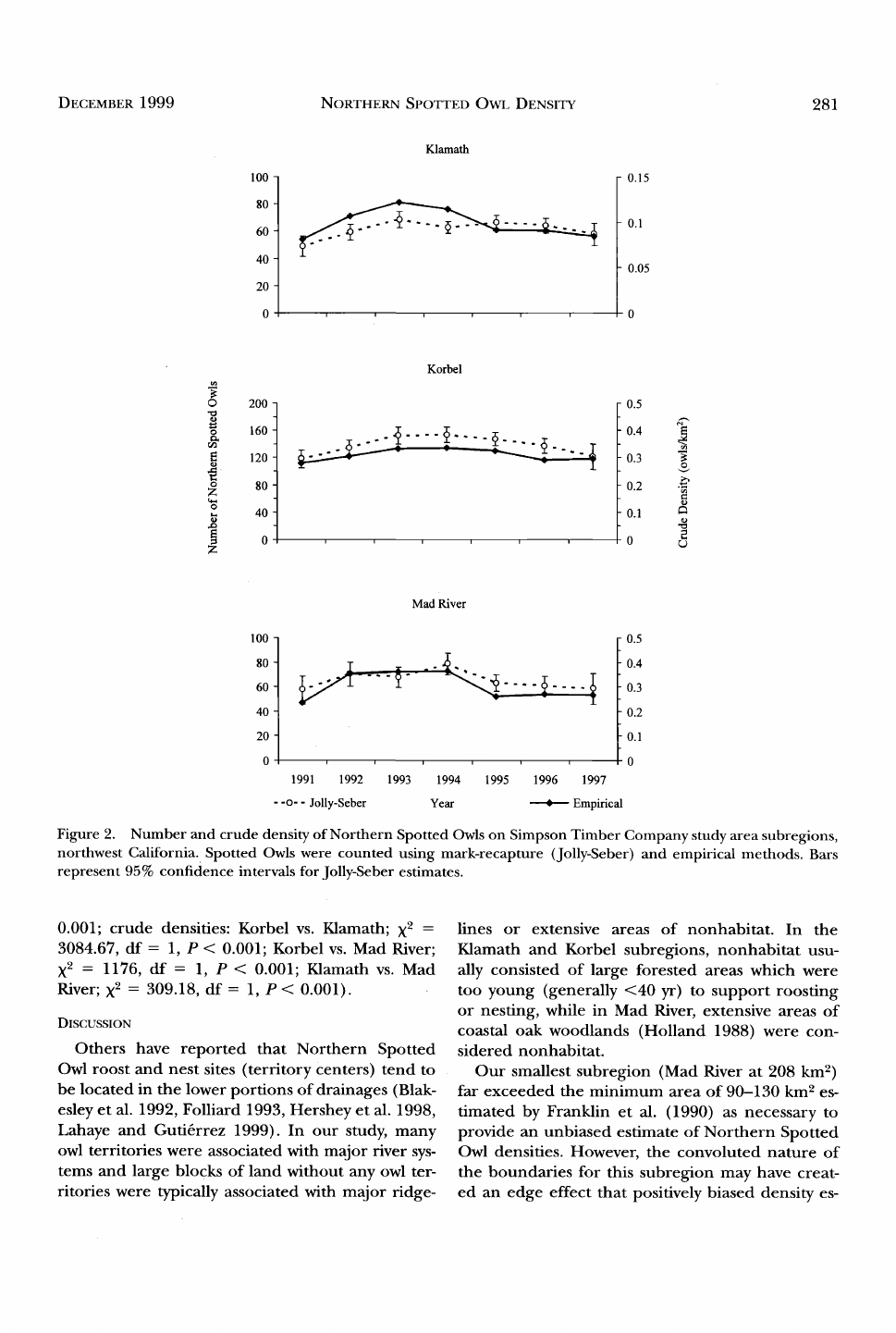
Abundance estimates appeared to increase over

the first two years of the study (Fig. 2). The overall

test of homogeneity for abundance estimates over

the seven years yielded significant differences for

Klamath (X 2 = 22.80, df = 6, P < 0.001), Korbel

(X 2 -- 27.49, df = 6, P < 0.001) and Mad River (X 2

= 14.14, df = 6, P = 0.028). The 1991 abundance

estimates for Klamath (48.91 -+ 3.65 [+-SE]) and

Korbel (117.24 +- 6.62) were significantly lower

than their mean estimates for the other years,

Table 4. Jolly-Seber estimates of capture probabilities

(P), apparent survival probabilities (qb) and percent co-

efficient of variation (CV) for mean abundance estimates

of Northern Spotted Owls for three subregions of the

Simpson Timber Company study area in northern Cali-

fornia, 1991-97.

SUBREGION P SE (P) qb SE (qb) CV (%)

Klamath 0.78 0.03 0.87 0.02 6.7

Korbel 0.84 0.01 0.88 0.01 3.1

Mad River 0.82 0.02 0.85 0.02 5.6

1992-97 (Klamath: • = 63.09 i 1.23; X 2 = 13.56,

df = 1, P < 0.001; and Korbel: i = 140.81 i 2.69;

X 2 = 10.88, df = 1, P = 0.001). The Mad River

abundance estimate for 1994 (78.50 i 4.67) was

significantly different from the mean estimate for

the other years (• = 62.82 -+ 2.00; X 2 = 9.52, df =

1, P = 0.002).'Bonferroni adjustments of the alpha

level prevented identifying additional significant

differences.

Empirical and J-S estimates of abundance

showed similar general trends for all subregions,

but there were some differences in individual es-

timates among some years. The confidence inter-

vals for J-S estimates did nbt overlap empirical es-

timates of the abundance during 1992-94, 1993-

96 and 1995 for Klamath, Korbel and Mad River,

respectively (Fig. 2). The mean empirical and J-S

estimates of abundance (Table 5) differed for Kor-

bel (X 2 = 6.805, df = 1, P = 0.009), but were not

significantly different for Klamath (X 2 -- 0.623, df

= 1, P = 0.430) or Mad River (X 2 = 0.792, df = 1,

P-- 0.373).

Mean J-S crude densities were highest for Korbel

followed by Mad River and Klamath (Table 5) with

an overall mean of 0.209 owls/km 2 (95% C.I. =

0.190-0.228). Ecological densities followed the

same trend as crude densities (Fig. 2) but calculat-

ed values were higher (Table 5). Comparisons of

mean crude and ecological densities indicated that

the three subregions were significantly different

for both variables (X 2 = 2038.098, df = 2, P <

0.001 and X •= 1249.670, df = 2, P < 0.001 for the

crude and ecological comparisons, respectively).

Post hoc comparisons showed crude and ecological

density estimates for all subregions to be different

from each other (Table 5, ecological densities: Kor-

bel vs. Klamath; X 2 = 4871.43, df = 1, P < 0.001;

Korbel vs. Mad River; X 2 = 38.35, df -- 1, P< 0.001;

Klamath vs. Mad River; X• = 1679.44, df = 1, P <

DECEMBER 1999 NORTHEed,• SPOTTED OWL DENSITY 281

lOO

Klamath

0.15

0.1

0.05

200

160

120

Korbel

0.5

0.4

0.3

0.2

0.1

Mad River

lOO

1991 1992 1993 1994 1995 1996 1997

--o-- Jolly-Seber Year * Empirical

0.5

0.4

0.3

0.2

0.1

Figure 2. Number and crude density of Northern Spotted Owls on Simpson Timber Company study area subregions,

northwest California. Spotted Owls were counted using mark-recapture (Jolly-Seber) and empirical methods. Bars

represent 95% confidence intervals for Jolly-Seber estimates.

0.001; crude densities: Korbel vs. Klamath; X 2 =

3084.67, df = 1, P < 0.001; Korbel vs. Mad River;

X 2 = 1176, df = 1, P < 0.001; Klamath vs. Mad

River; X 2 = 309.18, df = 1, P < 0.001).

DISCUSSION

Others have reported that Northern Spotted

Owl roost and nest sites (territory centers) tend to

be located in the lower portions of drainages (Blak-

esley et al. 1992, Folliard 1993, Hershey et al. 1998,

Lahaye and Gutifirrez 1999). In our study, many

owl territories were associated with major river sys-

tems and large blocks of land without any owl ter-

ritories were typically associated with major ridge-

lines or extensive areas of nonhabitat. In the

Klamath and Korbel subregions, nonhabitat usu-

ally consisted of large forested areas which were

too young (generally <40 yr) to support roosting

or nesting, while in Mad River, extensive areas of

coastal oak woodlands (Holland 1988) were con-

sidered nonhabitat.

Our smallest subregion (Mad River at 208 km 2)

far exceeded the minimum area of 90-130 km • es-

timated by Franklin et al. (1990) as necessary to

provide an unbiased estimate of Northern Spotted

Owl densities. However, the convoluted nature of

the boundaries for this subregion may have creat-

ed an edge effect that positively biased density es-

282 DtLLER AND THOME VOL. 33, NO. 4

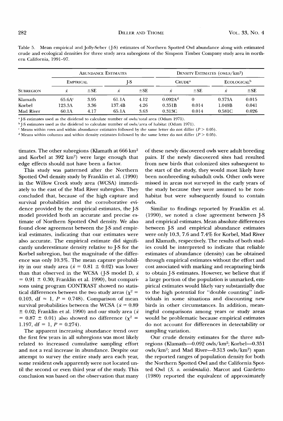
Table 5. Mean empirical and Jolly-Seber (J-S) estimates of Northern Spotted Owl abundance along with estimated

crude and ecological densities for three study area subregions of the Simpson Timber Company study area in north-

ern California, 1991-97.

ABUNDANCE ESTIMATES DENSITY ESTIMATES (owus/k•n 2)

EMPIRICAL J-S CRUDE a ECOLOGICAL b

SUBREGION • ----- SE • _+ SE • _+ SE / +-- SE

Klamath 65.6A c 3.95 61.1A 4.12 0.092A d 0 0.373A 0.015

Korbel 123.3A 3.36 137.4B 4.26 0.351B 0.014 1.049B 0.041

Mad River 60.1A 4.17 65.1A 3.63 0.313C 0.014 0.581C 0.026

aJ-S estimates used as the dividend to calculate number of owls/total area (Odum 1971).

bJ-S estimates used as the dividend to calculate number of owls/area of habitat (Odum 1971).

Means within rows and within abundance estimates followed by the same letter do not differ (P > 0.05).

Means within columns and within density estimates fbllowed by the same letter do not differ (P > 0.05).

timates. The other subregions (Klamath at 666 km '•

and Korbel at 392 km 2) were large enough that

edge effects should not have been a factor.

This study was patterned after the Northern

Spotted Owl density study by Franklin et al. (1990)

in the Willow Creek study area (WCSA) immedi-

ately to the east of the Mad River subregion. They

concluded that, because of the high capture and

survival probabilities and the corroborative evi-

dence provided by the empirical estimates, the J-S

model provided both an accurate and precise es-

timate of Northern Spotted Owl density. We also

found close agreement between the J-S and empir-

ical estimates, indicating that our estimates were

also accurate. The empirical estimate did signifi-

cantly underestimate density relative to J-S for the

Korbel subregion, but the magnitude of the differ-

ence was only 10.3%. The mean capture probabil-

ity in our study area (/= 0.81 _ 0.02) was lower

than that observed in the WCSA (J-S model D, •

= 0.91 -+ 0.30; Franklin et al. 1990), but compari-

sons using program CONTRAST showed no statis-

tical differences between the two study areas (X '• =

0.103, df = 1, P = 0.748). Comparison of mean

survival probabilities between the WCSA (• -- 0.89

+ 0.02; Franklin et al. 1990) and our study area (i

-- 0.87 + 0.01) also showed no difference (X •=

1.197, df = 1, P-- 0.274).

The apparent increasing abundance trend over

the first few years in all subregions was most likely

related to increased cumulative sampling effort

and not a real increase in abundance. Despite our

attempt to survey the entire study area each year,

some resident owls apparently were not located un-

til the second or even third year of the study. This

conclusion was based on the observation that many

of these newly discovered owls were adult breeding

pairs. If the newly discovered sites had resulted

from new birds that colonized sites subsequent to

the start of the study, they would most likely have

been nonbreeding subadult owls. Other owls were

missed in areas not surveyed in the early years of

the study because they were assumed to be non-

habitat but were subsequently found to contain

owls.

Similar to findings reported by Franklin et al.

(1990), we noted a close agreement between J-S

and empirical estimates. Mean absolute differences

between J-S and empirical abundance estimates

were only 10.3, 7.6 and 7.4% for Korbel, Mad River

and Klamath, respectively. The results of both stud-

ies could be interpreted to indicate that reliable

estimates of abundance (density) can be obtained

through empirical estimates without the effort and

cost associated with marking and recapturing birds

to obtain J-S estimates. However, we believe that if

a large portion of the population is unmarked, em-

pirical estimates would likely vary substantially due

to the high potential for "double counting" indi-

viduals in some situations and discounting new

birds in other circumstances. In addition, mean-

ingful comparisons among years or study areas

would be problematic because empirical estimates

do not account for differences in detectability or

sampling variation.

Our crude density estimates for the three sub-

regions (Klamath--0.092 owls/km2; Korbel--0.351

owls/km'•; and Mad River--0.313 owls/km '•) span

the reported ranges of population density for both

the Northern Spotted Owl and the California Spot-

ted Owl (S. o. occidentalis). Marcot and Gardetto

(1980) reported the equivalent of approximately

DECEMBER 1999 NORTHERN SPOTTED OWL DENSITY 283

0.325 owls/km '• in the Six Rivers National Forest

which is similar to our estimates for Korbel and

Mad River. However, as noted by Franklin et al.

(1990), their estimate was based on empirical

counts from night surveys without marking birds,

and their largest study area was only 58.2 km 2. Both

of these factors would likely positively bias their es-

timates making comparisons to this study problem-

atic. The lower population density in Klamath is

similar to many of the reported densities of Cali-

fornia Spotted Owls in the Sierra and San Berna-

dino Mountains (Roberts 1993, Moen and Guti6r-

rez 1993, Lahaye and Gutierrez 1994). Franklin et

al. (1990) provided the most rigorous estimate re-

ported for the population density of Northern

Spotted Owls. They estimated a density of 0.235

owls/km 2 for the 292 km '• WCSA, which was inter-

mediate in study area size between the Korbel and

Mad River subregions of our study. Their estimate

was similar to our combined estimate (0.209 owls/

km2), but less than either Korbel or Mad River,

which were located in closest proximity to the

WCSA. Tanner and Guti6rrez (1995) estimated

0.219 owls/km = for a 137.7 km '• study area in Red-

wood National Park, which was the only previous

estimate of density for Northern Spotted Owls in

the coastal redwood region. This was an empirical

estimate based on two years of surveys, but most

owls were marked, thus the estimate was likely ac-

curate.

Without other density studies in the coastal red-

wood region of Northern California, it is difficult

to know the extent to which this study is represen-

tative of the region. However, we believe the pat-

tern of density we observed was reflective of the

region in general. This was based on a qualitative

assessment we conducted using the 1996 California

Natural Diversity Database (G. Gould, California

Department of Fish and Game, unpubl. data) of

reported Northern Spotted Owl locations across

the entire range of the subspecies in California

and on unpublished data from an adjacent large

industrial land owner (S. Chinnici, Pacific Lumber

Company, pers. comm.).

There was a significant difference in the amount

of forested habitat in specific age classes among

the three subregions. We could only speculate on

how this might have influenced owl density since

the study was not designed to assess this. Although

some young stands (20-40 yr) in the STC study

area were associated with high Northern Spotted

Owl fecundity and low turnover rates, forests <40

yr old were not selected in proportion to their

availability by owls for nesting (Thorne et al. 1999).

Thus, high proportions of stands <40 yr old might

limit owl density. Klamath had significantly lower

densities of owls than the other subregions along

with the highest proportion of the landscape m

younger stands (83.7% <40 yr old). Klamath also

tended to have extensive areas of homogeneous

younger age classes, although we have not quanu-

fled this difference. In comparison, Korbel had

high densities of owls, with 64.3% of forest stands

<40 yr old. Based on extensive harvesting in the

last 10-15 yr with relatively small clearcuts (10-24

ha), Korbel tended to have a much more hetero-

geneous mixture of stand ages relative to Klamath.

In the same study area, Folliard (1993) noted that

landscapes supporting Northern Spotted Owls had

more edge and greater stand diversity than ran-

domly selected landscapes. Finally, like Korbel,

Mad River had high densities of owls, but only

28.7% of stands were <40 yr old. We had no data

to establish a direct cause and effect relationship

between habitat variables and the density of owls

in the different subregions and comparing density

to habitat variables was not the primary objective

of this study. However, as noted by Thome et al.

(1999), a combination of different age classes (old-

er stands for nesting and younger stands for for-

aging) may provide the best habitat for Northern

Spotted Owls in our region.

By definition, ecological densities are equal to or

greater than crude densities, and one can predict

that the magnitude of the difference will increase

as the proportion of habitat for a given species de-

creases on the landscape. Ecological densities were

4.05, 2.99 and 1.86 times higher than crude densi-

ties for Klamath, Korbel and Mad River, respectively,

which supported the predicted differences based on

the relative amounts of habitat in each region. In

comparison, Franklin et al. (1990) reported ecolog-

ical densities that were 2.81 and 2.31 times higher

than crude densities depending upon the approach

used for defining owl habitat.

It is difficult to make meaningful comparisons

of ecological densities among studies in different

areas unless the same criteria are used to calculate

ecological densities. Using mature/old-growth for-

ests to represent owl habitat, Franklin et al. (1990)

reported an ecological density of 0.660 owls/km '•

in the WCSA. Their estimate of ecological density

was greater than our estimate for the Klamath re-

gion (0.373 owls/km=), less than Korbel (1.049

284 D•LL}•R AND THOME VOL. 33, NO. 4

owls/km 2) but quite similar to Mad River (0.581

owls/km2). In addition to being closest in prox-

imity to the WCSA, Mad River also had the highest

proportion of mature stands (36.9% >80 yr in age,

although it lacked old growth habitat) compared

to 35.6% mature/old growth in the WCSA.

There is some question as to the extent compar-

isons of Northern Spotted Owl densities, either

w•thin or between study areas, can be used for de-

veloping management prescriptions. As noted by

Van Horne (1983), population density of a species

can be a misleading indicator of habitat quality.

Although some of the attributes of Northern Spot-

ted Owl populations do not meet the criteria for

habitat quality-density decoupling, a prediction

consistent with decoupling habitat quality and den-

sity is that high owl densities on selected managed

lands result from displacement of owls from adja-

cent harvested areas. However, we believe this was

unlikely because the densities in our study area ap-

peared to be relatively stable throughout a time

period when, due to its federally-listed status

(USDI 1992), significant habitat alteration of

Northern Spotted Owl habitat was not permitted

on adjacent private lands. In addition, there was a

90-95% reduction in annual timber harvest on ad-

jacent public land (Six Rivers National Forest) just

prior to and after the listing of the Northern Spot-

ted Owl (USDA 1995). Finally, we have observed

that the highest reproduction tends to be associ-

ated with areas of highest densities (L. Diller, un-

publ. data), but it was beyond the scope of this

study to quantify the relationship between repro-

duction and density.

Although it was unlikely that the densities of

owls in our study area were influenced by displace-

ment from adjacent areas, we could not assess hab-

itat quality in our study area based on density of

owls. First and foremost, we could not establish

causal relationships between the observed differ-

ences in density and corresponding differences in

habitat attributes without undertaking an experi-

mental approach over large areas. Correlative stud-

ies to elucidate patterns between habitat attributes

and density were not possible when only a few sub-

regions were available for comparison. In addition,

we could only estimate the density of the territorial

population of owls, and true density, which would

include nonterritorial floaters, was unknown. Giv-

en the difficulty of undertaking experiments with

a protected species over large areas, we believe that

more immediate insight can be gained concerning

habitat quality by relating demographic parameters

to habitat attributes in a manner described in

Thome et al. (1999). Ultimately, knowing popula-

tion density is of limited immediate benefit for de-

veloping conservation strategies for Northern

Spotted Owls without knowing the habitat attri-

butes that result in demographic parameters that

will sustain populations over time. However, estab-

lishing reliable estimates of population densities

for Northern Spotted Owls should provide valu-

able baseline data for assessing long-term trends in

their populations. Similar studies should be con-

ducted in selected areas throughout the range of

the Northern Spotted Owl to allow future assess-

ment of the long-term response of this species to

current management strategies now being imple-

mented.

ACKNOWLEDGMENTS

We thankJ.M. Beck, G.H. Brooks, D.E. Copeland, L.B

Folliard, K.H. Hamm, CJ. Hibbard, R.R. Klug, B.D. Mi-

chaels, D.B. Perry, J.L. Thompson, J.P. Verschuyl and BJ.

Yost for their exceptional fieldwork. G.N. Warinner and

C.J. Lane were very patient in helping with STC's GIS

data. K.H. Hamm provided valuable editorial review and

data analysis for the development of the manuscript. An

ß earlier draft was greatly improved by comments fromJ.B.

Buchanan, L.L. Irwin and an anonymous reviewer.

L•TERATURr C•TEr)

ANDERSON, D.R., K.P. BURNHAM AND G.C. WHITE. 1994.

AIC model selection in overdispersed capture-recap-

ture data. Ecology 75:1780-1793.

BART, J. AND E.D. FORSMAN. 1992. Dependence of North-

ern Spotted Owls Strix ocddentalis caurina on old-

growth forests in the western USA. Biol. Cons. 62:95-

100.

BLAKESLE¾, J.A., A.B. FRANKLIN AND RJ. GUTieRReZ. 1992.

Spotted Owl roost and nest-site selection in north-

western California. J. Wildl. Manage. 56:388-392.

BURNHAM, K.P., D.R. ANDERSON, G.C. WHITE, C. BROWNIE

AND K.H. POLLOCK. 1987. Design and analysis meth-

ods for fish survival experiments based on release-re-

capture. Am. Fish. Soc. Monogx 5.

CAR•¾, A.B., J.A. RE•D AND S.P. HORTON. 1990. Spotted

Owl home range and habitat use in southern Oregon

Coast Ranges. J. Wildl. Manage. 54:11-17.

--, S.P. HORTON AND B.L. B•SWELL. 1992. Northern

Spotted Owls: influence of prey base and landscape

character. Ecol. Monogx 62:223-250.

CAUGHLEY, C-. AND A. S•NCLAIR. 1994. Wildlife ecology and

management. Blackwell Scientific Publications, Cam-

bridge, MA U.S.A.

ELFOre), R.C. 1974. Climate of Humboldt and Del Norte

counties. Humboldt and Del Norte Counties Agric.

Exten. Serv., Univ. California, Davis, CA U.S.A.

DECEMBER 1999 NORTHERN SPOTTED OWL DENSITY 285

FOLLIARD, L.B. 1993. Nest-site characteristics of Northern

Spotted Owls in managed forests of northwest Cali-

fornia. M.S. thesis, Univ. Idaho, Moscow, ID U.S.A.

FORSMAN, E.D. 1981. Molt of the Spotted Owl. Auk 98:

735-742.

1983. Methods and materials for locating and

studying Spotted Owls. USDA For. Serv. Gen. Tech.

Rep. PNW-162, Portland, OR U.S.A.

ß 1988. A survey of Spotted Owls in young forests

in the northern coast range of Oregon. Murrelet 69:

65-68.

, E.C. MESLOW AND MJ. S•:RUB. 1977. Spotted Owl

abundance in young versus old-growth forests. Oreg.

Wildl. Soc. Bull. 5:43-47.

--, --AND --. 1984. Distribution and biol-

ogy of the Spotted Owl in Oregon. Wildl. Monog½. 87:

1-64.

, C.R. BRUCE, M.A. WALKER AND E.C. MESLOW.

1987. A current assessment of the Spotted Owl pop-

ulation in Oregon. Murrelet 68:51-54.

, A.B. FRANKLIN, F.M. OLIVER AND J.P. WARD. 1996.

A color band for Spotted Owls. J. Field Ornithol. 67:

507-510.

FRANKLIN, A.B., J.P. WArn), RJ. GUTII•RREZ AND G.I.

GOULD, JR. 1990. Density of Northern Spotted Owls

in northwest California. J. Wildl. Manage. 54:1-10.

GUTIERREZ, RJ., E.D. FORSMAN, A.B. FRANKLIN AND E.C.

MESLOW. 1996, History of demographic studies in the

management of the Northern Spotted Owl. Stud. Ari-

an Biol. 17:6-11.

HERSHEY, K.T, E.C. MESLOW AND F.L. P,•USEY. 1998. Char-

acteristics of ibrests at Spotted Owl nest sites in the

Pacific Northwest. J. Wildl. Manage. 62:1398-1410.

HINES, J.W. AND J.R. S^UER. 1989. Program CONTRAST--

A general program for the analysis of several survival

or recovery rate estimates. USDI Fish and Wildl. Serv.,

Tech. Rep. 24. Washington, DC U.S.A.

HIN•:ZE, J.L. 1997. NCSS 97: Statistical system for win-

dows. NCSS, Kaysville, UT U.S.A.

HOLLAND, V.L. 1988. Coastal oak woodland. Pages 78-79

in K.E. Mayer and W.F. Laudenslayer, Jr. [EDs.], A

guide to wildlife habitats of California. USDA Forest

Service, Sacramento, CA U.S.A.

INTERGRAPH CORPORATION. 1994. MGE base mapper ref-

erence manual. Intergraph, Huntsville, AL U.S.A.

JOLLY, G.M. 1965. Explicit estimates from capture-recap-

ture data with both death and immigration-stochastic

model. Biometrika 52:225-247.

1982. Mark-recapture models with parameters

constant in time. Biometrics 38:301-321.

KI•BS, C.J. 1985. Ecology: the experimental analysis of

distribution and abundance. Harper and Row, New

York, NY U.S.A.

LAHAY•, W.S. AND RJ. GUTII•RREZ. 1994. Big Bear Spotted

Owl study, 1993. Calif. Dept. of Fish and Game, Non-

game Bird and Mammal Section. Tech. Rep. 1994-3,

Sacramento, CA U.S.A.

--AND --'. 1999. Nest sites and nesting habitat

of the Northern Spotted Owl in northwestern Cah-

fornia. Condor 101:324-330.

LEBKETON, J.-D., K.P. BURNH^M, J. CLOBERT AND D.R. AN-

DERSON. 1992. Modeling survival and testing biologi-

cal hypotheses using marked animals: a unified ap-

proach with case studies. Ecol. Monogr. 62:67-118.

MARCOT, B.G. ANDJ. GARDETTO. 1980. Status of the Spot-

ted Owl in Six Rivers National Forestß West. Birds 11'

79-87ß

--AND J.W. THOMAS. 1997. Of Spotted Owls, old

growth, and new policies: a history since the Inter-

agency Scientific Committee Reportß USDA For. Serv.

Gen. Tech. Rep. PNW-408, Portland, OR UßSßAß

MA•ER, K.E. 1988. Redwoodß Pages 60-61 in K.E. Mayer

and W.F. Laudenslayer, Jr. [EDs.], A guide to wildlife

habitats of California, USDA Forest Service, Sacra-

mento, CA U.S.A.

MCCULLAGH, P. AND J.A. NELDER. 1989. Generalized hn-

ear models. Chapman and Hall, New York, NY U.S.A.

MOEN, C.A., A.B. FP,2',NKLIN AND RJ. GUTIgRP, EZ. 1991. Age

determination of subadult Northern Spotted Owls tn

northwest California. Wildl. Soc. Bull. 19:489-493.

--AND R.J. GUTII•RREZ. 1993. Population ecology of

the California Spotted Owl in the central Sierra Ne-

vada: annual results, 1992. Calif. Dept. of Fish and

Game, Nongame Bird and Mammal Section. Tech.

Rep. 1993-14, Sacramento, CA U.S.A.

NETER, J. AND W. WASSERMAN. 1974. Applied linear staus-

tical modelsß Richard D. Irwin, Homewood, IL U.S.A

ODUM, E.P. 1971. Fundamentals of ecology. Saunders Col-

lege Publ., Philadelphia, PA U.S.Aß

POLLOCK, K.H.,J.E. HINES ANDJ.D. NICHOLS. 1985. Good-

ness-of-fit tests for open capture-recapture models

Biometrics 41: 399-410.

, J.D. NICHOLS, C. BROWNIE AND J.E. HINES. 1990.

Statistical inference for capture-recapture experi-

ments. Wildl. Monogz. 107:1-97.

ROBERTS, C.K. 1993. California Spotted Owl (Strix occiden-

talis caurina) inventory and demographic study, Se-

quoia and Kings Canyon National Parks: final 1988-

89. Calif. Dept. of Fish and Game, Nongame Bird and

Mammal Section. Tech. Rep. 1993-4, Sacramento, CA

U.S.A.

SAUER, RJ. AND B.K. WILLIAMS. 1989. Generalized pro-

cedures for testing hypotheses about survival or re-

covery rates. J. Wildl. Manage. 53:137-142.

SEBER, G.A.E 1965. A note on the multiple recapture cen-

sus. Biometrika 52:249-259.

ß 1982. The estimation of animal abundance and

related parameters. Charles Griffin and Co., London,

U.K.

SIMPSON TIMBER COMPANY. 1992. Habitat conservauon

plan for the Northern Spotted Owl on the Califorma

timberlands of Simpson Timber Company. Simpson

Timber Company, Korbel, CA U.S.A.

SOLIS, D.M., JR. AND RJ. GUTII•RREZ. 1990. Summer hab-

286 D•LI•E}• AND THOME VOL. 33, NO. 4

itat ecology of Northern Spotted Owls in northwest-

ern California. Condor 92:739-748.

TaN•4E}•, R.G. HI) RJ. GUTI•P,J•Z. 1995. A partial inven-

tory of Northern Spotted Owls (Strix occidentalis caur-

ina) in Redwood National Park, 1994. Unpubl. Rep.,

Arcata, CA U.S.A.

THOM^S, J.W., E.D. FORSMAN, J.B. LINT, E.C. MESI•OW,

B.R. NOO•4 aNI)J. VEP, NE}•. 1990. A con'servation strat-

egy for the Northern Spotted Owl. U.S. Gov. Printing

Off., Washington, DC U.S.A.

THOME, D.M., C.J. Z•mEL aND L.V. DILLEP,. 1999. Forest

stand characteristics and reproduction of Spotted

Owls in managed north-coastal California forests. J.

Wildl. Manage. 63:44-59.

USDA. 1995. Land and resource management plan for

the Six Rivers National Forest: final environmental im-

pact statement. Eureka, CA U.S.A.

USDI. 1992. Draft recovery plan for the Northern Spot-

ted Owl. USDI Fish and Wildl. Serv., Portland, OR

U.S.A.

V^N HORNE, B. 1983. Density as a misleading indicator

of habitat quality. J. Wildl. Manage. 47:893-901.

ZINI•, PJ. 1988. The redwood forest and associated north

coast forests. Pages 679-698 in M.G. Barbour and J.

Major [EI)s.], Terrestrial vegetation of California.

Univ. of Calif. Davis, Davis, CA U.S.A.

Received 28 January 1999; accepted 24 July 1999