What's Your Favorite Color? Controlling the Appearance of a Graph

PharmaSUG 2020 - Paper DV-006

What's Your Favorite Color?

Controlling the Appearance of a Graph

Richann Watson, DataRich Consulting

ABSTRACT

The appearance of a graph produced by the Graph Template Language (GTL) is controlled

by Output Delivery System (ODS) style elements. These elements include fonts and line and

marker properties as well as colors. A number of procedures, including the Statistical

Graphics (SG) procedures, produce graphics using a specific ODS style template. This paper

provides a very basic background of the different style templates and the elements

associated with the style templates. However, sometimes the default style associated with a

particular destination does not produce the desired appearance. Instead of using the default

style, you can control which style is used by indicating the desired style on the ODS

destination statement. However, sometimes not a single one of the 50-plus styles provided

by SAS® achieves the desired look. Luckily, you can modify an ODS style template to meet

your own needs. One such style modification is to control which colors are used in the

graph. Different approaches to modifying a style template to specify colors used are

discussed in depth in this paper.

INTRODUCTION

The appearance of many SAS-generated visualizations is controlled by ODS style elements.

There are over 50 different ODS styles that can be used for ODS statistical graphics. These

styles determine things such as the font, background color, the wall color, grouping color,

and contrasting color, just to name a few. Each ODS destination has a default style

associated with it. However, sometimes the default styles do not meet our needs. We may

have a client that wants things in black and white but with a specific font, so using the

standard colors associated with a style that utilizes that font may not be feasible. Or we

may need to have a consistent set of colors for specific values, thus allowing SAS to set the

colors may not be ideal. Because companies or individuals have different views on what

they deem as an ideal look for a graph, SAS allows for customization of styles. You can

write your own style, or you can start with a style that has most of the components you like

and modify that style to fit your needs. This paper will focus on taking existing styles and

modifying specific elements to create the desired look within GTL. However, these concepts

can be applied to other types of visualizations.

UNDERSTANDING ODS STYLES AND ELEMENTS

Before you can write your own style, it is advisable to have a basic understanding of the

different styles and some of the elements associated with styles. In this paper, we will

touch briefly on some of the different style elements, with the primary focus being adjusting

the colors.

DEFAULT STYLES AND COMMON ODS STYLES

For each device and ODS destination, SAS has default styles. For example, the default style

for the PDF destination is the “Pearl” style template, and the default style for the RTF

destination is the “RTF” style template (Figures 1 and 2).

Figure 1: Sample Figure with STYLE =

Pearl

Figure 2: Sample Figure with STYLE =

RTF

A list of default styles for each ODS destination and device combination can be found at

Default Devices and Styles for Commonly Used ODS Destinations. If you are curious as to

how each of these styles would look in HTML, PDF and RTF, you can run the SAS code that

is found at Program for Viewing Multiple Styles.

However, you are not limited to using the default style for the indicated destination and

device. There are over 50 styles that are part of SAS that you can choose from. Refer to the

ODS Styles Gallery for a list of the various styles available in SAS.

Below are some recommended SAS-supplied style templates:

• DEFAULT

• HTMLBLUE

• ANALYSIS

• DAISY

• JOURNAL

• JOURNAL2

• JOURNAL3

• STATISTICAL

A complete list of recommended style templates can be found at Recommended Styles for

ODS Destinations.

What makes these styles different? They can vary based on font style, font size, and font

color. They can also vary based on fill color, background color and a variety of other style

elements as demonstrated in Figures 3 – 6 and Appendix 1.

Figure 3: Sample Figure for Style =

DEFAULT

Figure 4: Sample Figure for Style =

HTMLBLUE

Figure 5: Sample Figure for Style =

ANALYSIS

Figure 6: Sample Figure for Style =

DAISY

To see more samples of the various styles visit Statistical Graphics Using ODS: ODS Styles

Comparisons.

COMMON ODS STYLE ELEMENTS

SAS has a set of common ODS style elements that are used to produce most graphs. For

example, GraphDataDefault, GraphData1 – GraphDatan, GraphConfidence as well as others.

These common ODS style elements have pre-set values for various attributes, such as the

marker size and symbol, line style and thickness, and color that are dependent on the style

specified.

With most of the SAS defined styles, there is an inheritance from a parent style. For

example, ANALYSIS style inherits most of its style elements from the DEFAULT style. In

addition, DAISY inherits from the HTMLBLUE style which inherits from the STATISTICAL

style and the STATISTICAL style inherits from the DEFAULT style. When one style inherits

from another style only the elements that are different are specified.

GraphData1 – GraphDatan are attributes that are specifically related to the grouped data

item associated with the indicated number. For example, GraphData1 are the attributes

associated with the first grouped data item, while GraphData4 are attributes associated with

the fourth grouped data item.

How these various pre-defined ODS style elements are displayed is dependent on the ODS

style used, as shown in Figures 7 – 10 and Appendix 2. Notice that for the Figures 7 – 10

that regardless of the type of graph that is displayed that if the colors are not specified for

each grouped data that SAS will use the pre-defined elements associated with GraphDatan

for each nth group.

For example, if you view the differences between the styles for Figures 7 and 9 you will

notice that the primary difference is the colors. For DEFAULT and ANALYSIS styles,

GraphData1 uses the circle as the marker with a line pattern of 1 (solid line); GraphData2

uses the plus sign as the marker with a line pattern of 4 (medium dash); and GraphData3

uses an ‘X’ as the marker with a line pattern of 8 (MediumDashShortDash). However, as

noted in Output 1 the colors are different. In Figures 8 and 10, you will notice that for all

three groups the same marker and line pattern are used but as illustrated in Output 1 they

too have different colors.

DEFAULT and ANALYSIS use the default rotation pattern which means that it will use the

markers, line patterns, and colors associated with the corresponding GraphDatan. However,

HTMLBLUE and DAISY (prior to SAS 9.4M6) used the color-priority as the default rotation.

Note that starting with SAS 9.4M6 DAISY style will use the default rotation pattern instead

of the color-priority rotation.

Output 1: Color Codes GraphData1 – GraphData3 for DEFAULT, HTMLBLUE, ANALYSIS and

DAISY styles

Figure 7: Sample Figures for Some

Common ODS Style Elements for Style

= DEFAULT

Figure 8: Samples Figure for Some

Common ODS Style Elements for

STYLE = HTMLBLUE

CX7C95CA CXDE7E6F CX66A5A0 CX6F7EB3 CXD05B5B CX66A5A0

RGB(124, 149, 202) RGB(222, 126, 111) RGB(102, 165, 160) RGB(111, 126, 179) RGB(208, 91, 91) RGB(102, 165, 160)

CX8FB38F CXF2AE49 CXB49C6A CX3D5AAE CX90B328 CX9D2E14

RGB(143, 179, 143) RGB(242, 174, 73) RGB(180, 156, 106) RGB(61, 90, 174) RGB(144, 179, 40) RGB(157, 46, 20)

DEFAULT

ANALYSIS

DAISY

HTMLBLUE

Figure 9: Sample Figures for Some

Common ODS Style Elements for Style =

ANALYSIS

Figure 10: Sample Figures for Some

Common ODS Style Elements for Style =

DAISY

Most of the styles use DEFAULT as the parent style. Each style definition inherits attributes

from the parent style (e.g., DEFAULT) and specifies the attributes for the element(s) that

are different from the parent.

For more common ODS Style Elements visit Statistical Graphics Using ODS: Some Common

ODS Style Elements.

IDENTIFYING COLORS

Millions of colors are available for use when creating the necessary output. These colors can

be specified within SAS using one of the seven valid color-naming schemes.

• RGB (red green blue)

• CMYK (cyan magenta yellow black)

• HLS (hue lightness saturation)

• HSV (hue saturation brightness), also called HSB

• Gray scale

• SAS color names (from the SAS Registry)

• SAS Color Naming System (CNS)

Although there are millions of colors theoretically at our disposal, it does not mean that all

the colors are available. There are limitations to the number of colors that can be displayed

for given devices and/or media types. The device you are using will determine the number

of colors that can be processed and viewed, as not all devices have the capability to display

all the possible colors specified for an output. If a specific color is not available, then SAS

and the device use an existing color that is a close approximation of the desired color.

Refer to the RGB and HLS values needed for SAS in Table 1.

Table 1 illustrates a couple of examples of what the color scheme value is for the specific

color as well as the value in SAS that corresponds to the indicated color scheme value.

Color-Naming

Scheme

Example for

Pink

Value Specified

in SAS

Example for

Turquoise

Value Specified

in SAS

RGB (red green

blue)

255, 192, 203

CXFFC0CB

CXFFBFCC ♯

64, 225, 208

CX40E0D0

CX40E0D1 ♯

CMYK (cyan

magenta yellow

black) †

0, 25, 20, 0

CMYK00403300

71, 0, 7, 12

B500121F

HLS (hue

lightness

saturation)

349, 87, 99

H06DE0FF

H06EDFFF ‡

123, 144, 184

H12690B8

H12590B8 ‡

HSV (hue

saturation

brightness), also

called HSB

348, 24, 100

V15C3DFF

173, 71, 87

V0ADB5DE

Gray scale

(255+192+203)

GRAYD8

(64+224+208)

GRAYA5

SAS color names

(from the SAS

Registry)

Pink

Turquoise

SAS Color Naming

System (CNS) ╫

Very light vivid

purplish red

Verylightvividpur

plishred

Light moderate

blue green

Light_moderate_

blue_green

♯ HEX code returned when %RGB macro is used. Although this is slightly different than the one in the

SAS registry it yields a color that is nearly identical to the one provided by the HEX code in the list of

predefined colors in the SAS registry.

† If the value returned from %CMYK macro starts with a number, then the CMYK number used when

specifying the color must start with ‘CMYK’. Otherwise, the ‘CMYK’ prefix is not required.

‡ HLS code returned when %RGB2HLS macro is used. Although this is slightly different than the one in

the SAS registry, it yields a color that is nearly identical to the one provided in the list of predefined

colors in the SAS registry.

╫ Although the colors do not match exactly with the RGB color, it is pretty close. When specifying a

color using CNS, you can either remove spaces between each component or separate each

component with an underscore.

Table 1: Color-Naming Schemes and Example Values

Assume you have the RGB decimal code (i.e., the values for R, G, and B), how do you

convert that to a value that can be used by SAS? If you know the RGB values, you can

easily retrieve the HEX code for each corresponding color element by using the HEX2

format, as illustrated in SAS Program 1. Data Display 1 shows the output from the program

and provides the corresponding HEX code for pink and turquoise.

The selection of colors is beyond the scope of the paper, but it is worth mentioning that

there are a number of things to take under consideration when choosing colors: including

the number of colors or shades needed for a color ramp; and whether the foreground and

background are different enough so that someone who is color blind can distinguish

between the different components. Sites such ADA Compliance Site which can help with

determining colors for color blind, while you can use the ColorBrewer2 to help choose

colors, gray scale equivalents, and color ramps.

data color_convert;

set color;

rgbhex = cats("CX", put(r, hex2.), put(g, hex2.), put(b, hex2.));

gray = (r + g + b) / 3;

grayhex = put(gray, hex2.);

rper = round(r/255*100);

gper = round(g/255*100);

bper = round(b/255*100);

run;

SAS Program 1: Determining HEX code

COLOR

RGBHEX

GRAY

GRAYHEX

RPER

GPER

BPER

pink

255

192

203

CXFFC0CB

216.6667

100

turquoise

224

208

CX40E0D0

165.3333

Data Display 1: RGB and Gray HEX Codes

In addition, there are several color SAS-defined utility macros that can help determine the

code that should be used when specifying a color in SAS. %COLORMAC can be executed in

order to compile all the SAS color utility macros. SAS Program 2 demonstrates some of the

color utility macros.

Note that for %RGB macro, the individual color 255-based values need to be converted to a

percentage. SAS Program 1 shows how R, G, and B are converted to percentages of 255.

The last three columns in Data Display 1 show the converted values, which are used in the

%RGB macro in SAS Program 2. For more information on these utility macros visit Using

Color Utility Macros.

data _null_;

put "PINK RGB: %RGB(100, 75, 80)";

put "PINK RGBtoHLS: %RGB2HLS(CXFFC0CB)";

put "PINK HSV: %HSV(348, 24, 100)";

put "PINK CMYK: " %CMYK(0, 25, 20, 0);

put "TURQ RGB: %RGB(25, 88, 82)";

put "TURQ RGBtoHLS: %RGB2HLS(CX40E0D0)";

put "TURQ HSV: %HSV(174, 71, 87)";

put "TURQ CMYK: " %CMYK(71, 0, 7, 12);

run;

SAS Program 2: Determining SAS Value for Different Color-Schemes

If you are unsure of the what the hue, saturation, light or brightness are for a specific HEX

code, you can use a color converter tool such as the one found at this website

https://www.rapidtables.com/convert/color/.

For more information on specifying colors visit Color-Naming Schemes.

MODIFYING THE COLORS

As mentioned earlier the primary focus is going to be on changing the colors, but similar

concepts illustrated for changing the colors can be applied for changing the font size, font

style, marker size, line size and pattern. There are several ways to change the colors.

UNDERSTANDING ROTATION PATTERN

For each style there are attributes that are rotated through for grouped data. The attributes

which are rotated through are determined based on the GraphDatan style element for the

indicated style that is being used. Understanding the attribute rotation pattern is important

to ensuring that the any grouped data is represented by the correct set of attributes.

ATTRPRIORITY option on the ODS GRAPHICS statement or in BEGINGRAPH statement can

be used to override the default rotation pattern. By default, ATTRPRIORITY is set to “AUTO”

which allows the specific style used to determine the rotation pattern. ATTRPRIORITY =

“COLOR” is known as a color-priority style or all-color style which indicates that the colors

should be rotated through prior to rotating through the other attributes such as marker

symbols and line patterns. When the attributes are rotated through it is based on the order

of the data. Therefore, if you need to have colors appear in a specific order then either the

colors need to be specified in the order in which they would appear in the data or the data

needs to be sorted so that the data order is in alignment with the order in which the colors

are specified.

SPECIFYING COLOR ON BEGINGRAPH STATEMENT

One of the easiest ways to change a color for all graphs within a template and have it

applied to all plot statements within the template is to specify the fill color and/or contrast

color on the BEGINGRAPH statement.

SAS Program 3 demonstrates the use of two options that allow you to specify the colors.

proc template;

define statgraph bplot1;

begingraph / border = false

datacolors = (pink plum paleturquoise)

datacontrastcolors = (black);

layout overlay / xaxisopts = (label = " "

type = discrete)

yaxisopts = (label = "Number of Patients with Event");

barchart x = trtan y = event / orient = vertical group = trtan

barlabel = true;

endlayout;

endgraph;

end;

run;

SAS Program 3: Modifying Color within Graph Template Using BEGINGRAPH

Options

On the BEGINGRAPH statement, there are several options available that will allow you to

control the attributes. You can specify the fill colors to replace the colors associated with

the GraphDatan style elements by using DATACOLORS. A color for each group should be

specified. DATACONTRASTCOLORS is used to specify the contrast colors that are to be

used. Colors are used for fill areas while the contrast colors are used for the markers and

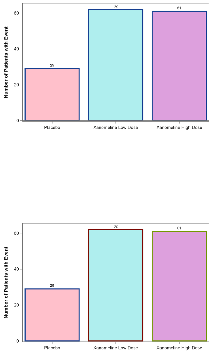
outlines. In Figure 11, you can see that each bar corresponds to one of the colors in the

DATACOLORS option and the lines for each bar is black which corresponds to the color

indicated in DATACONTRASTCOLORS. However, notice that the order in which the colors

are listed: pink, plum, paleturquoise; but Figure 11 has pink, paleturquoise and plum. This

is due to the fact that in the data, Xanomeline High Dose appears prior to Xanomeline Low

Dose. If Xanomeline Low Dose should be plum, then the data should be sorted

appropriately or the list on the DATACOLORS option should be reordered. If we sort the

data by so that Placebo records come first, followed by Xanomeline Low Dose with

Xanomeline High Dose last and re-render the template, then the colors would be as

expected (Figure 12).

Figure 11: Modifying Color within Graph Template Using BEGINGRAPH Options –

Rendering Graph without Sorting

Figure 12: Modifying Color within Graph Template Using BEGINGRAPH Options –

Sorting Data Prior to Rendering Graph

If there are not enough colors specified on the DATACOLORS option (SAS Program 4) to

account for all the unique groups, then two additional sets of colors will be automatically

created. The two additional sets of colors are generated based on the original colors

specified. The first set is a shade lighter and the second set is a shade darker as illustrated

by Figure 13.

proc template;

define statgraph bplot4;

begingraph / border = false

datacolors=(pink)

datacontrastcolors=(black);

layout overlay / xaxisopts = (label = " "

type = discrete

yaxisopts = (label = "Number of Patients with Event");

barchart x = trtan y = event / orient = vertical group = trtan

barlabel = true;

endlayout;

endgraph;

end;

run;

SAS Program 4: Modifying Color within Graph Template Using BEGINGRAPH

Options – Specifying Only One Color

Figure 13: Modifying Color within Graph Template Using BEGINGRAPH Options –

Specifying Only One Color

MANUALLY ASSIGNING ON PLOT STATEMENT

Another quick way to change a color is to assign the color directly on the corresponding plot

statement. The options to modify the colors will vary based on the type of graph and

whether or not the data is grouped (i.e., GROUP option is used).

Applying One Color

SAS Program 5 illustrates the syntax needed to change all the bar charts to one color.

Notice that in this example the bar chart is one color and the line around the bar chart is

another color (Figure 14).

proc template;

define statgraph bplot1;

begingraph / border = false;

entrytitle textattrs = (color = pink) "All Barcharts One Color";

layout overlay / xaxisopts = (label = " " type = discrete)

yaxisopts = (label = "Number of Patients with Event");

barchart x = trtan y = event / orient = vertical group = trtan

fillattrs = (color = pink)

outlineattrs = (color = deeppink)

barlabel = true;

endlayout;

endgraph;

end;

run;

SAS Program 5: Modifying Color within Graph Template to One Color – BARCHART

FILLATTRS controls the color of the filled area of the bars while OUTLINEATTRS controls the

color of the line around the bars. The default color for non-grouped data is based on

GraphDataDefault for the filled area and based on GraphOutlines for the bar outlines. For

grouped data the color is based on the GraphData1 – GraphDatan for both the filled bars

and bar outlines.

Figure 14: Modifying Color within Graph Template to One Color - BARCHART

SAS Program 6 shows the syntax needed to change the colors for all the series plots to one

color. In this example, we demonstrate that the markers and the line can be two different

colors. The color of the marker is controlled by the MARKERATTRS statement and the color

for the line is controlled by LINEATTRS statement. We can also control the color of the

labels for the x and y axes.

Note that this is for illustration purposes only. Typically, this method is used when there is

only one series to be plotted (i.e., GROUP option is not used).

proc template;

define statgraph wtseries1;

begingraph / border = false;

layout overlay / xaxisopts = (label = 'Weeks'

labelattrs = (color = black weight = bold)

linearopts = (viewmin = 0 viewmax = 26))

yaxisopts = (label = 'Mean Weight (kg)'

offsetmin = 0.07

offsetmax = 0.07

labelattrs = (color = deeppink weight = bold)

linearopts = (viewmin = 63 viewmax = 72));

seriesplot x = avisitn y = mean / display = all group = trtan

markerattrs = (symbol = circlefilled

color = pink

size = 6)

lineattrs = (color = deeppink

pattern = 34

thickness = 3);

endlayout;

endgraph;

end;

run;

SAS Program 6: Modifying Color within Graph Template to One Color - SERIESPLOT

The marker is the symbol that is used to represent each point on the series plot. Within the

MARKERATTRS option there are various other options that can be defined to meet the

desired output needs. One such element is the color. As shown in Figure 15 the markers

are filled pink circles.

Similar to markers, the line that connects the markers can have attributes that can be

customized. In this example, we are using a deep pink dotted line to connect the pink filled

circles that have a size of 6.

Figure 15: Modifying Color within Graph Template to One Color - SERIESPLOT

Notice that in Figure 15 that the legend does not provide any additional information since

the markers and colors are the same for all three groups. Typically, when displaying

grouped data, you need some attribute that distinguishes the data, such as color. It is

possible to use an all-color style but have other attributes to help differentiate; however,

the focus of this paper is illustrating the different ways to color. Note that the treatment

values were manually inserted to help discern between the treatments.

Applying a Color Gradient or Color List

But what if we do not want everything to be one color? How do we assign the colors when

the GROUP option is used?

SAS Program 7 uses the COLORMODEL and COLORRESPONSE options to control the colors

for the graphs.

proc template;

define statgraph bplot2;

begingraph / border = false;

entrytitle textattrs = (size = 11 pt color = pink) "Placebo";

entrytitle textattrs = (size = 11 pt color = hotpink) "Low Dose";

entrytitle textattrs = (size = 11 pt color = deeppink) "High Dose";

layout overlay / xaxisopts = (label = " " type = discrete)

yaxisopts = (label = "Number of Patients with Event");

barchart x = trtan y = event / orient = vertical group = trtan

colorresponse = trtan

colormodel = (pink hotpink deeppink)

barlabel = true;

endlayout;

endgraph;

end;

run;

SAS Program 7: Modifying Color within Graph Template to Different Colors –

BARCHART

Attributes for entry titles can also be controlled using TEXTATTRS option. Figure 16

demonstrates that the colors for the ENTRYTITLE can be modified by using the TEXTATTRS

= (COLOR = color) option.

The COLORMODEL specifies a color ramp. The COLORMODEL can use either a color-ramp

style element or a color list. A color-ramp style element consists of a STARTCOLOR,

NEUTRALCOLOR and ENDCOLOR. This color-ramp style element is used to create a

continuous color gradient. SAS Program 7 shows the use of a color list for the

COLORMODEL.

If COLORMODEL is used, then either COLORRESPONSE or COLORBYFREQ option needs to be

used. For this example, the COLORRESPONSE option is used and it is tied to the GROUP

option. The COLORRESPONSE represents which variable will be used to map the fill area of

the bar chart based on the color model.

Figure 16 illustrates the results of using the COLORMODEL and COLORRESPONSE options in

the template.

Figure 16: Modifying Color within Graph Template to Different Colors - BARCHART

USING A DISCRETE ATTRIBUTE MAP

An attribute map can be created that will help control various style elements, such as text

attributes, line attributes and marker attributes, which includes the colors. The use of an

attribute map can be created within the template or as an external data set. In addition,

the referencing of the attribute map can also be done within the template or when the

template is rendered.

Within a Graph Template

With the use of an attribute map, you can ensure that specific values will have a consistent

color across various outputs that use that specific template regardless of what ODS style is

used and regardless if the data source has all the data available. For example, if we want

‘Placebo’ to always be pink and ‘Xanomeline Low Dose’ to always be hot pink and

‘Xanomeline High Dose’ to always be deep pink when this particular graph is produced, then

if the data source is missing a treatment it will still maintain the color scheme which is

defined in the attribute map. SAS Program 8 and Figure 17 illustrates the use of a discrete

attribute map within the graph template.

SAS Program 8: Modifying Color using Discrete Attribute Map Defined Within

Graph Template

The DISCRETEATTRMAP statement is used to create an attribute map within the graph

template. It allows the user to specify various attributes, such as color, for each formatted

data value. If a data value is formatted, then the formatted value must be used in the

attribute map. DISCRETEATTRMAP must be placed inside the template between the

BEGINGRAPH statement and the first LAYOUT statement. There are three main components

of the attribute map.

• The first is the initialization of the map. This is where the attribute map is provided a

name. In SAS Program 8 the attribute map is referred to as “TRTCOLOR”. When

naming the attribute map, several options can also be specified, such as

IGNORECASE, TRIMLEADING and DISCRETELEGENDENTRYPOLICY.

• The second part is defining the attributes for one or more formatted data value

using the VALUE statement. With the VALUE statement things like color and line

options can be defined for each formatted data value that is to have a specific set of

attributes. If two or more values have the same set of attributes, rather than

defining the attributes for each value, all the values sharing the same attributes can

be on the same VALUE line with each individual value enclosed in its own set of

quotation marks and separated by a blank space. Refer to SAS Program 9 for how

the DISCRETEATTRMAP would be set up when multiple values share the same

proc template;

define statgraph bplot3;

begingraph / border = false;

entrytitle textattrs = (size = 11 pt color = black)

"DISCRETEATTRMAP Defined in Template";

discreteattrmap name = "TRTCOLOR";

value "Placebo" / fillattrs = (color = pink)

lineattrs = (color = black);

value "Xanomeline Low Dose" / fillattrs = (color = hotpink)

lineattrs = (color = black);

value "Xanomeline High Dose" /fillattrs = (color = deeppink)

lineattrs = (color = black);

enddiscreteattrmap;

discreteattrvar attrvar = colorvar var = trtan attrmap = "TRTCOLOR";

layout overlay / xaxisopts = (label = " "

type = discrete)

yaxisopts = (label = "Number of Patients with Event");

barchart x = trtan y = event / orient = vertical

group = colorvar

barlabel = true;

endlayout;

endgraph;

end;

run;

attribute (Figure 18). The value statement can have OTHER (not in quotes) to create

a category of all other values that are not specified. If OTHER is not specified, then

those data values that do not have a VALUE statement will have attributes assigned

as if there were no attribute map.

• The last component is to signal the end of the attribute map definition, which is done

with ENDDISCRETEATTRMAP.

Once the attribute map is defined, then the attributes need to be associated with the

corresponding variable. In addition, the association must be provided a name for reference

within the template. DISCRETEATTRVAR statement is used in order to make this

association. In SAS Program 8, “TRTCOLOR” attribute map is associated with the variable

TRTAN and the association is named COLORVAR.

The association name assigned on the DISCRETEATTRVAR statement is then specified in the

appropriate plot statement.

Figure 17: Modifying Color using Discrete Attribute Map Defined Within Graph

Template

discreteattrmap name = "TRTCOLOR";

value "Placebo" /

fillattrs = (color = pink) lineattrs = (color = black);

value "Xanomeline Low Dose" "Xanomeline High Dose" /

fillattrs = (color = deeppink) lineattrs = (color = black);

enddiscreteattrmap;

SAS Program 9: Modifying Color using Discrete Attribute Map Defined Within

Graph Template with Multiple Values Having Same Attributes

Figure 18: Modifying Color using Discrete Attribute Map Defined Within Graph

Template with Multiple Values Having Same Attributes

Within a Data Set

There may be situations where a particular color scheme may need to be used across

various types of graphs. In these cases, defining the attribute map within the template is

not ideal because it would need to be defined in each graph template that is created. In

order to reuse an attribute map, it can be stored in a data set that can be referenced when

the graph template is rendered.

When creating a data set for the attribute mapping, it needs to contain an ID which has a

value that is equivalent to the name that the attribute map would be assigned if using

DISCRETEATTRMAP within the graph template. In addition, the data set needs to have a

record for each possible formatted value that has specific attributes. The data set only

needs to contain the necessary fields that are needed for the specific attributes that are to

be associated with the value. For example, if you only need the color scheme to create bar

charts then only FILLCOLOR and LINECOLOR are needed. However, if the color scheme will

be used for other types of graphs such as a series plot, then other fields, such as

MARKERCOLOR, need to be included. SAS Program 10 demonstrates how an attribute map

can be created as a permanent data set. With this permanent data set, the color scheme

can be reused. Notice that more than one color scheme can be stored within an attribute

map data set. They are distinguishable by the ID (Table 2).

data ADAM.ATTRMAP (drop = i j);

array idvr(2) $9 _TEMPORARY_ ('TRTCOLOR' 'TRTCOLOR2');

array vals(3) $25 _TEMPORARY_ ('Placebo' 'Xanomeline Low Dose'

'Xanomeline High Dose');

array clrs(2, 3) $20 _TEMPORARY_ ('Pink' 'HotPink' 'DeepPink'

'Turquoise' 'MediumTurquoise' 'DarkTurquoise');

do i = 1 to 2;

ID = idvr(i);

do j = 1 to 3;

VALUE = vals(j);

FILLCOLOR = clrs(i, j);

LINECOLOR = clrs(i, j);

MARKERCOLOR = clrs(i, j);

output;

end;

run;

SAS Program 10: Creating an Attribute Map as a Permanent Data Set

VALUE

FILLCOLOR

LINECOLOR

MARKERCOLOR

TRTCOLOR

Placebo

Pink

TRTCOLOR

Xanomeline Low Dose

HotPink

TRTCOLOR

Xanomeline High Dose

DeepPink

TRTCOLOR2

Placebo

Turquoise

TRTCOLOR2

Xanomeline Low Dose

MediumTurquoise

TRTCOLOR2

Xanomeline High Dose

DarkTurquoise

Table 2: ATTRMAP Data Set

When the attribute map is stored in a data set, there is no need to use the

DISCRETEATTRMAP statement as illustrated in SAS Program 8. However, the

DISCRETEATTRVAR statement is still needed in order to associate the attributes with the

corresponding variable. After the attribute map data set is created it needs to be associated

with the graph template and the data. This is done using the DATTRMAP option on

SGRENDER procedure (SAS Program 11).

proc sgrender data = adtte template = bplot4

dattrmap = ADAM.ATTRMAP;

format trtan trt.;

run;

SAS Program 11: Specifying Attribute Map Data Set on PROC SGRENDER

Figure 19: Creating an Attribute Map as a Permanent Data Set and Specifying

Attribute Map on PROC SGRENDER

Notice that in Figure 19 it looks slightly different than the figure that is produced by SAS

Program 8 (Figure 17). This is because in SAS Program 8 the outline of the bar charts was

set to black, while the outline in the attribute map data set matches the color of the

corresponding bar. By creating the data set we can update the attribute map without having

to update the graph template(s). If you wish for the outlines to be black similar to what

shown in Figure 17, then LINECOLOR in Table 2 would be changed to ‘Black’ instead of

matching the value in FILLCOLOR.

Even though an attribute map data set was created, the use of DISCRETEATTRVAR was still

needed. However, this can also be removed, and an association can be made at the time of

rendering, which allows different color schemes to be implemented using the same template

(SAS Program 12).

proc sgrender data = adtte template = bplot5

dattrmap = ADAM.ATTRMAP;

dattrvar trtan = 'TRTCOLOR';

format trtan trt.;

run;

proc sgrender data = adtte template = bplot5

dattrmap = ADAM.ATTRMAP;

dattrvar trtan = 'TRTCOLOR2';

format trtan trt.;

run;

SAS Program 12: Associating the Attribute Map with Corresponding Variable on

PROC SGRENDER

DATTRVAR is used to associate the variable with the corresponding attribute map name.

The attribute map name must exist in the attribute map data set and must be enclosed in

quotes when specified on the DATTRVAR statement. Note that if there is more than one plot

defined in the template and each plot has attributes defined in the attribute map data set,

then DATTRVAR statement would list all possible variable assignments (separated by a

space) needed for rendering the graph with the specific template.

With the use of the DATTRVAR, it allows the attributes to be changed for the graph without

changing the template (Figure 20).

Figure 20: Illustration of use of DATTRVAR to Change Attributes

Thus, with the use of DATTRMAP and DATTRVAR, an attribute map data set can be used on

any graph template that has the indicated values as demonstrated in SAS Program 13 and

Figure 21.

proc sgrender data = meanwt template = wtseries3 dattrmap = ADAM.ATTRMAP;

dattrvar trtan = 'TRTCOLOR';

format trtan trt.;

run;

proc sgrender data = meanwt template = wtseries3 dattrmap = ADAM.ATTRMAP;

dattrvar trtan = 'TRTCOLOR2';

format trtan trt.;

run;

SAS Program 13: Reuse of Attribute Map Data Set and Different Attribute Maps

Figure 21: Reuse of Attribute Map Data Set and Different Attribute Maps

For more details on using attributes map refer to Using Attribute Maps.

CREATING YOUR OWN STYLE

Typically, when dealing with styles, you start with an existing one rather than writing one

from scratch due to the complexity. Thus, you can view the many styles that SAS offers

and determine which one is close to what you want but may require the modification of a

few of the elements. There are several ways to modify an existing style.

If you wish to view the source code that is associated with a particular style template, you

can run the following code (SAS Program 14). This will write the code used to produce that

style to the log.

proc template;

source STYLES.DAISY;

run;

SAS Program 14: Viewing Source Code for Style Template

Using the Style Template Modification Macro

The easiest way to update an existing style is to use the style template modification macro,

%MODSTYLE. It allows you to customize the style elements that govern the appearance of

group observations. There are several parameters that can be specified, such as NAME,

PARENT, COLORS, FILLCOLORS, and more. For parameters that are not specified when the

macro is called these the default values will be used. Refer to Style Template Modification

Macro for full details. SAS Program 15 demonstrates how the macro can be specified.

%modstyle(name = mystyle1,

parent = default,

colors = black black black,

fillcolors = pink plum paleturquoise)

…

ods pdf dpi = 300 file="&outdir.modified_barchart_mystyle1.pdf" style = mystyle1;

SAS Program 15: Modifying Style Using %MODSTYLE

NAME parameter allows you to specify the name for the new style that you are creating. If

NAME is not provided, then the new style name will default to NEWSTYLE.

PARENT parameter indicates what style the newly created style should inherit the majority

of its attributes from. If PARENT is not provided, then the parent style will default to

DEFAULT. Since the default parent style is DEFAULT, then it is not necessary to specify

PARENT = DEFAULT. It is only done in SAS Program 15 for illustration purposes.

COLORS parameter contains one or more colors that are space delimited. The colors

specified are used for markers and lines. If the COLORS option is not used, then the colors

from the parent style are used.

FILLCOLORS parameter is the color list that is used for bands and fill areas (e.g., bar

charts). Note that the number of colors listed in FILLCOLORS needs to be same number of

colors specified in COLORS. If there are more colors listed in FILLCOLORS, then any extra

colors will be ignored. Notice that for FILLCOLORS there are three colors specified,

therefore, three colors needed to be specified on the COLORS parameter, even if all the

colors are the same there needs to be three colors in the color list. If FILLCOLORS is not

provided, then the fill colors from the parent style are used.

On the ODS statement, the STYLE = option can be used to specify the name of the style

that was created. Without the STYLE = option, SAS will use the default style for the

indicated destination.

Figure 22 illustrates the results of using %MODSTYLE (SAS Program 15). The DEFAULT was

the parent style thus we have the grey background. The fill area for the bar charts were

changed from blue, red, and green to pink, plum, and pale turquoise. In addition, the bar

outlines were changed from blue, red, and green to black for all three.

Figure 22: Modifying Style Using %MODSTYLE

Using STYLE Statement in TEMPLATE Procedure

There are other methods for modifying the elements of an existing style without having to

use the macro. Recall that with the %MODSTYLE there are default values for some of the

parameters if they are not specified. If you do not want to use the default values from the

style template modification macro but do not want to specify all the parameters (or are not

sure how to specify them), then you can use TEMPLATE procedure.

SAS Program 16 and SAS Program 17 provide two examples of how to modify an existing

style.

proc template;

define style mystyle2;

parent = STYLES.DAISY;

style GraphOutlines from GraphOutlines / linethickness = 3;

style GraphData1 / color = pink;

style GraphData2 / color = plum;

style GraphData3 / color = paleturquoise;

end;

run;

SAS Program 16: Modifying Style Using STYLE Statement in PROC TEMPLATE –

Example 1

When customizing an existing style, you will need to provide it a style name. The style

name cannot overwrite an existing SAS style. By default, any style created or modified will

be saved to the SASUSER.TEMPLAT area. However, if you want to make the style available

to others, you can save it to a permanent location by modifying the ODS PATH statement

(refer to SAS Program 17).

For the data being used there are three groups and we want the colors for each group to be

different than what is in the parent style, but everything else for each group to be

consistent. This is known as an ‘all-color’ style (or ‘color-priority’ style). In other words, we

want the attribute rotation to go through the colors first.

An ‘all-color’ style is when the other attributes are the same (e.g., line pattern, marker) and

only the color is used to distinguish between the groups until all the colors for the style is

exhausted then it recycles the colors with a different marker or line pattern. For example, in

a bar chart, the line color and pattern remain the same until all the colors in a style is used.

Once all the colors are used then the line color and/or pattern changes and then goes

through the cycle of colors again. This cycle repeats until all groups in the data have been

accounted for.

In order to achieve an ‘all-color’ style, we use the STYLE statement to redefine GraphData1,

GraphData2, GraphData3. With the STYLE statement specified as in SAS Program 16 only

the attribute for color is defined. All other attributes that would be associated with

GraphData1 – GraphData3 would default to non-grouped data attribute.

libname ADAM "C:\Users\gonza\Desktop\Conferences\What is Your Favorite Color\Data";

ods path ADAM.TEMPLAT (update) SASUSER.TEMPLAT (read) SASHELP.TMPLMST (read);

proc template;

define style mystyle3;

parent = STYLES.DAISY;

style GraphOutlines from GraphOutlines / linethickness = 3;

style GraphData1 from GraphData1 / color = pink;

style GraphData2 from GraphData2 / color = plum;

style GraphData3 from GraphData3 / color = paleturquoise;

end;

run;

SAS Program 17: Modifying Style Using STYLE Statement in PROC TEMPLATE –

Example 2

In order to save the modified style to a permanent location so that others can use, the ODS

PATH statement needs to be updated so that it lists the location of where the new style

should reside. The order in which the template stores are specified is the order in which

SAS will search. If no modification is made to the ODS PATH, then SAS will search in

SASUSER.TEMPLAT first and then SASHELP.TMPLMST. The UPDATE option allows new

templates to be written to that template store as well as allowing templates to be read from

it. In SAS Program 17, the new style is written to a permanent location and this permanent

location will be the first template store that is searched when looking for a specific template.

Notice that the STYLE statements in SAS Program 17 are very similar to SAS Program 16.

The difference is that for GraphData1, GraphData2, and GraphData3 the ‘from GraphDatan’

is used to indicate that the attributes are inherited from the parent style and only the

attribute specified is modified.

The best way to understand the difference between SAS Program 16 and SAS Program 17 is

to view the graphs. For purpose of illustration, the bar chart outlines were made to have a

line thickness of 3 so that they are easier to see, thus making it easier to see the difference

between the styles.

Figure 23 is generated from SAS Program 16 and Figure 24 is generated from SAS Program

17.

Figure 23: Modifying Style Using STYLE Statement in PROC TEMPLATE – Example 1

Notice in Figure 23 that the outline around each bar is blue. This is because MYSTYLE2 is an

‘all-color’ style; and GraphData1, GraphData2, and GraphData3 were redefined to only

specify the color attribute. Therefore, the outlines for the bars defaulted to the first color in

the parent style which is blue.

In Figure 24, the outlines for each bar correspond to the outlines of the original style

element. This is because when creating MYSTYLE3 it inherited the attributes from the

corresponding GraphDatan element and only the fill area color was overwritten. Unlike in

MYSTYLE2 where the entire style element was overwritten.

Figure 24: Modifying Style Using STYLE Statement in PROC TEMPLATE – Example 2

The use of the COLORRESPONSE and COLORMODEL options was previously introduced when

we wanted to specify the list of colors. But the COLORMODEL can be more than just a list

of colors, it can be used to determine a color gradient. SAS Program 18 demonstrates how

to create a color ramp using style template.

proc template;

define style mygradient;

parent=styles.daisy;

class twocoloraltramp /

startcolor = deeppink

endcolor = darkturquoise;

end;

run;

ods pdf style = mygradient;

proc sgplot data = hgt_wgt;

scatter x = wgt y = hgt / colorresponse = hgt

colormodel = twocoloraltramp

markerattrs = (symbol = circlefilled size = 8);

xaxis label = 'Mean Weight (kg)';

yaxis label = 'Mean Height (cm)';

run;

SAS Program 18: Modifying Color within Using a ColorRamp

To define a custom color gradient, you can overwrite the color ramp that is part of an

existing style. There are four pre-defined color ramps: TWOCOLORRAMP,

TWOCOLORALTRAMP, THREECOLORRAMP, THREECOLORALTRAMP. For the two-color ramp,

you only need to specify STARTCOLOR and ENDCOLOR. But for the three-color ramp, you

need to also specify NEUTRALCOLOR. With a color gradient, SAS will determine the colors

between the smallest color (STARTCOLOR) and the largest color (ENDCOLOR). If

NEUTRALCOLOR is provided, then this will be the mid-point color. The new color ramp is

defined in style template by using a parent style and just overwriting the necessary color

ramp. The color ramps with ‘ALT’ in the name are used for markers and plot lines, while the

ones without ‘ALT’ in the name are used for fill areas. Since the graph that is being

produced with Figure 25 is a scatter plot, then only the TWOCOLORALTRAMP is used

because there are only markers and plot lines; there are no fill areas.

In order to use the color ramp that is defined with the new style, you need to specify the

name of the new style on the ODS statement with STYLE option.

When using COLORMODEL, you can specify a color gradient. Prior to defining the template

for the graph, the DAISY template was modified to change the color ramp. This modified

color ramp is specified on the COLORMODEL statement.

Figure 25: Modifying Color within Using a ColorRamp

Using CLASS Statement in TEMPLATE Procedure

In addition to using the style template modification macro and the STYLE statement within

PROC TEMPLATE, you can modify the colors using the CLASS statement. Refer to SAS

Program 19 and SAS Program 20.

proc template;

define style mystyle4;

parent = STYLES.DAISY;

class GraphOutlines / linethickness = 3;

class GraphData1 / color = pink;

class GraphData2 / color = paleturquoise;

class GraphData3 / color = plum;

end;

run;

SAS Program 19: Modifying Style Using CLASS Statement in PROC TEMPLATE –

Example 1

Like the examples that used the STYLE statement, the goal is to modify the colors for the

three groups so that it is different than what was in the parent style. The code is very

similar to SAS Program 16 with the difference being that SAS Program 19 uses CLASS

instead of STYLE. So, what makes them different? Recall in SAS Program 16, it produced

an ‘all-color’ style for all other attributes that were not modified in the PROC TEMPLATE.

Thus, GraphData1 – GraphData3 were redefined. However, with the use of the CLASS

statement it is only modifying the attribute specified and inheriting the rest of the attributes

from the parent element. The CLASS statement works in the same manner as using the

STYLE statement with the FROM clause. In other words, the CLASS statement implies the

FROM, thus CLASS statement is the same as using the STYLE statement with the FROM

clause. They both inherit from the parent element. Notice that Figure 26 looks the same as

Figure 24.

Figure 26: Modifying Style Using CLASS Statement in PROC TEMPLATE – Example 1

Since the filled area of the bar charts had a color change it only makes sense to have a

color change for the outlines of the bars. This can also be achieved using the CLASS

statement or the STYLE statement with the FROM clause.

proc template;

define style mystyle4;

parent = STYLES.DAISY;

class GraphOutlines / linethickness = 3;

class GraphData1 / color = pink

contrastcolor = deeppink;

class GraphData2 / color = paleturquoise

contrastcolor = darkturquoise;

class GraphData3 / color = plum

contrastcolor = purple;

end;

run;

SAS Program 20: Modifying Style Using CLASS Statement in PROC TEMPLATE –

Example 2

While the COLOR option on the CLASS statement controls the color for the filled area of the

bar charts, the CONTRASTCOLOR option is used to indicate what colors are used for the

outline of the bar. Refer to Figure 27.

Figure 27: Modifying Style Using CLASS Statement in PROC TEMPLATE – Example 2

For more details on creating a style template visit TEMPLATE Procedure: Creating a Style

Template

CONCLUSION

You are not limited to using the pre-defined styles and/or pre-defined color schemes

associated with those styles. You can customize your graphs to meet your needs. There

are several different ways in which the colors can be modified. The option you choose is

dependent on whether you plan to reuse the color scheme for other graphs or if it is a one-

time use. Have fun coloring!

REFERENCES

Carpenter, Art. 2016. “Controlling Colors by Name; Selecting, Ordering, and Using Colors

for Your Viewing Pleasure.” Proceedings of SAS Global Forum 2016. Las Vegas, NV.

https://support.sas.com/resources/papers/proceedings16/4003-2016.pdf

CDISC. (2013). CDISC. Retrieved from SDTM/ADaM Pilot Project:

http://www.cdisc.org/system/files/members/article/application/zip/updated_pilot_submissio

n_package.zip

Color Conversion. https://www.rapidtables.com/convert/color/

Haworth, Lauren. 2002. “SAS® with Style: Creating your own ODS Style Template.”

Proceedings of SUGI 27. Orlando, FL: SAS Institute, Inc.

https://support.sas.com/resources/papers/proceedings/proceedings/sugi27/p186-27.pdf

Heath, Dan, 2018. “Diving Deep into SAS® ODS Graphics Styles.” Proceedings of

PharmaSUG 2018. Seattle, WA: PharmaSUG.

https://www.pharmasug.org/proceedings/2018/DV/PharmaSUG-2018-DV02.pdf

29 
 
Matange, Sanjay and Dan Heath. 2019. “Create A Combined Graph of Tumor Data.” 
Proceedings of SAS Global Forum 2019. Dallas, TX: SAS Institute, Inc. 
https://www.sas.com/content/dam/SAS/support/en/sas-global-forum-
proceedings/2019/3143-2019.pdf 
Smith, Kevin. 2006. “The TEMPLATE Procedure Styles: Evolution and Revolution.” 
Proceedings of SUGI 31. San Francisco, CA: SAS Institute, Inc. 
https://support.sas.com/resources/papers/proceedings/proceedings/sugi31/053-31.pdf 
Watson, Richann. 2019. “Great Time to Learn GTL: A Step-by-Step Approach to Creating 
the Impossible.” Proceedings of SAS Global Forum 2019. Dallas, TX: SAS Institute, Inc. 
https://www.sas.com/content/dam/SAS/support/en/sas-global-forum-
proceedings/2019/3170-2019.pdf  
Watts, Perry. 2003. “Working with RGB and HLS Color Coding Systems in SAS® Software”. 
Proceedings of SUGI 28. Seattle, WA: SAS Institute, Inc. 
https://support.sas.com/resources/papers/proceedings/proceedings/sugi28/234-28.pdf 
ACKNOWLEDGMENTS 
Thank you to Louise Hadden for always helping me with coming up with that ‘perfect’ word 
or phrase that helps clarify a concept. Thanks to Dan Heath for patiently answering all my 
questions.  I would also like to thank Kriss Harris for his thorough review of the content and 
providing valuable feedback. 
RECOMMENDED READING 
Hadden, Louise, et.al. 2007 “Color Your World – With SAS®.” Proceedings of NESUG 2007. 
Baltimore, MD. https://www.lexjansen.com/nesug/nesug07/po/po11.pdf 
Haworth, Lauren. 2006. “PROC TEMPLATE: The Basics.” Proceedings of SUGI 31. San 
Francisco, CA. 
https://support.sas.com/resources/papers/proceedings/proceedings/sugi31/112-31.pdf 
Kuhfeld, Warren. Basic ODS Graphics Examples. Free download, 
http://support.sas.com/documentation/prod-p/grstat/9.4/en/PDF/odsbasicg.pdf  
Kuhfeld, Warren. Advanced ODS Graphics Examples. Free download, 
https://support.sas.com/documentation/prod-p/grstat/9.4/en/PDF/odsadvg.pdf  
Lafler, Kirk Paul. “Making Your SAS® Results, Reports, Tables, Charts and Spreadsheets 
More Meaningful with Color.” Proceedings of MWSUG 2018. Indianapolis, IN. 
http://mwsug.org/proceedings/2018/SP/MWSUG-2018-SP-2.pdf 
Matange, Sanjay. Getting Started with the Graph Template Language in SAS®, SAS 
Institute (SAS Press, 2013).  
Matange, Sanjay. Clinical Graphs Using SAS®, SAS Institute (SAS Press, 2016).  
Rosanbalm, Shane. 2016. “Fifty Ways to Change your Colors (in ODS Graphics).” 
Proceedings of PharmaSUG 2016. Denver, CO. 
https://www.pharmasug.org/proceedings/2016/DG/PharmaSUG-2016-DG04.pdf 
   

30 
 
SAS REFERENCE LINKS 
Default Devices and Styles for Commonly Used ODS Destinations 
https://documentation.sas.com/?docsetId=graphref&docsetTarget=n03ikif9nd0pyin1nege0k
kwpmhu.htm&docsetVersion=9.4&locale=en 
Program for Viewing Multiple Styles 
https://documentation.sas.com/?docsetId=odsug&docsetTarget=p0lieqehqf2axgn148b3axe
cx9pe.htm&docsetVersion=9.4&locale=en 
ODS Styles Gallery 
https://documentation.sas.com/?docsetId=odsadvug&docsetTarget=p14qidvs5xf7omn14om
mvsuhvmzn.htm&docsetVersion=9.4&locale=en 
Recommended Styles for ODS Destinations 
https://documentation.sas.com/?docsetId=odsug&docsetTarget=n13ivejjjk8flyn1jajj8onc3x
nw.htm&docsetVersion=9.4&locale=en 
Statistical Graphics Using ODS: ODS Style Comparisons 
https://documentation.sas.com/?cdcId=pgmsascdc&cdcVersion=9.4_3.4&docsetId=statug&
docsetTarget=statug_odsgraph_sect059.htm&locale=en 
Statistical Graphics Using ODS: Some Common ODS Style Elements 
https://documentation.sas.com/?cdcId=pgmsascdc&cdcVersion=9.4_3.4&docsetId=statug&
docsetTarget=statug_odsgraph_sect058.htm&locale=en 
Processing Limitations for Colors 
https://documentation.sas.com/?docsetId=graphref&docsetTarget=n089voiecrvtcfn1outxa6
ta2l7x.htm&docsetVersion=9.4&locale=en 
Color Utility Macros 
https://documentation.sas.com/?docsetId=graphref&docsetTarget=n0e07qe1e8eapon1l4wk
cimup7wt.htm&docsetVersion=9.4&locale=en 
Color-Naming Schemes 
https://documentation.sas.com/?cdcId=pgmsascdc&cdcVersion=9.4_3.2&docsetId=grstatu
g&docsetTarget=p0edl20cvxxmm9n1i9ht3n21eict.htm&locale=en# 
Using Attribute Maps 
https://documentation.sas.com/?cdcId=pgmsascdc&cdcVersion=9.4_3.2&docsetId=grstatu
g&docsetTarget=p0wv2bbjftizkpn1puokmcblrw15.htm&locale=en 
Style Template Modification Macro (%MODSTYLE) 
https://support.sas.com/documentation/cdl/en/statug/63347/HTML/default/viewer.htm#sta
tug_odsgraph_sect056.htm 
TEMPLATE Procedure: Creating a Style Template 
https://documentation.sas.com/?docsetId=odsproc&docsetTarget=p1g9uebd55he4on1b213
etlcn3jo.htm&docsetVersion=9.4&locale=en 
Controlling Appearance of Grouped Data 
https://documentation.sas.com/?docsetId=grstatug&docsetTarget=p0q22l1wyqkxodn1kpxw
ez8dd7td.htm&docsetVersion=9.4&locale=en#n03nz7ce6fq43bn1186lwcdyc74i 

Predefined Colors

https://documentation.sas.com/?cdcId=pgmsascdc&cdcVersion=9.4_3.2&docsetId=grstatu

g&docsetTarget=n161ukdyz9wpfsn1nh8sihforvyq.htm&locale=en

Font Lists

https://documentation.sas.com/?docsetId=graphref&docsetTarget=n0c8945h7o2kmrn1h0u

ehmio2i6j.htm&docsetVersion=9.4&locale=en

Available Line Patterns

https://documentation.sas.com/?cdcId=pgmsascdc&cdcVersion=9.4_3.2&docsetId=grstatu

g&docsetTarget=n13pm0ndse66l2n1u309543mx2yt.htm&locale=en

Attributes Available for the Attribute Options

https://documentation.sas.com/?cdcId=pgmsascdc&cdcVersion=9.4_3.2&docsetId=grstatu

g&docsetTarget=p0yjbi9rz0z03tn1arz9ia9tgvic.htm&locale=en#n1xcsyjlynhepdn1liqenqamp

cp0

Marker Attributes and Symbols

https://documentation.sas.com/?docsetId=grstatproc&docsetTarget=p0i3rles1y5mvsn1hrq3

i2271rmi.htm&docsetVersion=9.4&locale=en

CONTACT INFORMATION

Your comments and questions are valued and encouraged. Contact the author at:

Richann Watson

DataRich Consulting

richann.watson@datarichconsulting.com

Any brand and product names are trademarks of their respective companies.

APPENDIX 1: ADDITIONAL SAMPLES OF COMMON ODS STYLES

APPENDIX 2: ADDITIONAL SAMPLES OF COMMON ODS STYLE

ELEMENTS