Summary of Stream Habitat and Fish Inventories on the

Summary of Stream Habitat Inventories on the Blue Ridge and Chattooga

River Districts of the Chattahoochee National Forest, Georgia 2014

United States Department of Agriculture Forest Service

Southern Research Station

Center for Aquatic Technology Transfer

1710 Research Center Drive

Blacksburg, VA 24060-6349

C. Andrew Dolloff, Team Leader

Report prepared by:

Colin Krause and Craig Roghair

September 2015

Table of Contents

Introduction ................................................................................................................................................... 2

Methods ........................................................................................................................................................ 3

Site Selections and Reach Layout ............................................................................................................ 3

Habitat Inventory ...................................................................................................................................... 3

Results ........................................................................................................................................................... 4

Depth and Width ....................................................................................................................................... 5

Habitat Area.............................................................................................................................................. 5

% Fines and Substrate .............................................................................................................................. 5

Large Wood .............................................................................................................................................. 6

Hemlock Abundance and Condition......................................................................................................... 6

Discussion ..................................................................................................................................................... 6

Data Availability ........................................................................................................................................... 7

Literature Cited ............................................................................................................................................. 7

Appendix A: Field Methods for Stream Habitat Inventory ....................................................................... 51

List of Figures

Figure 1. Streams inventoried on the Chattahoochee National Forest, Georgia. ......................................... 9

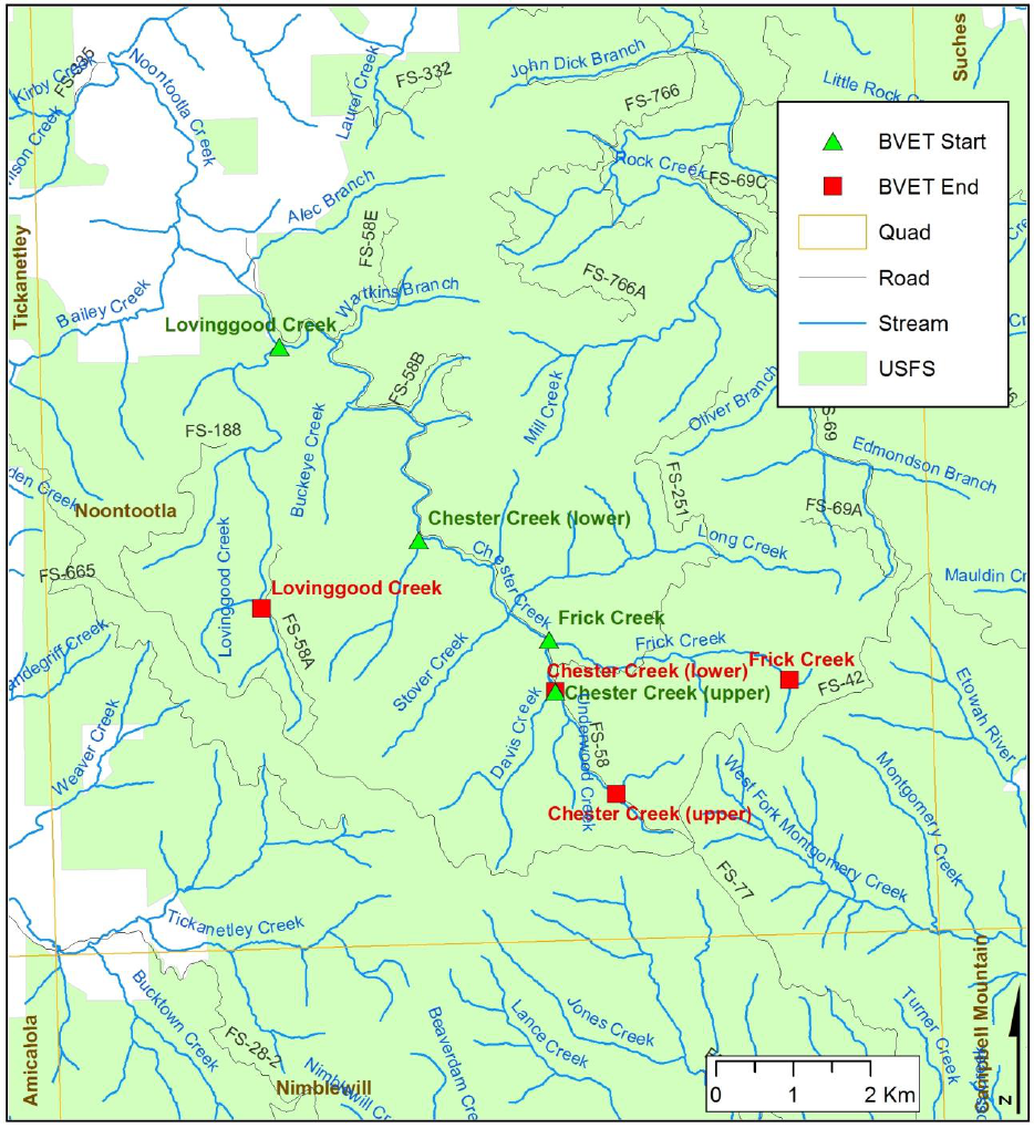
Figure 2. BVET inventory start and end locations on Lovinggood Creek, Chester Creek, and Frick Creek

on the Chattahoochee National Forest, Georgia. ........................................................................................ 10

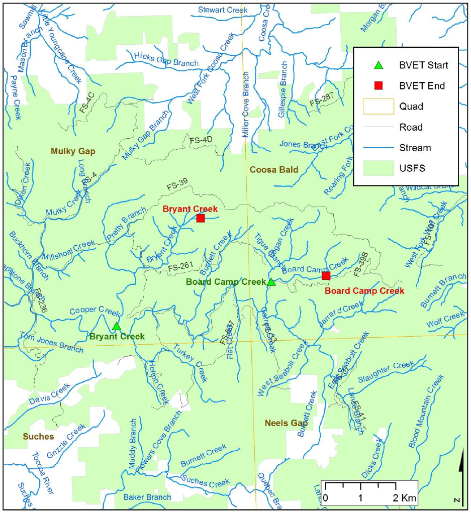
Figure 3. BVET inventory start and end locations on Bryant Creek and Board Camp Creek on the

Chattahoochee National Forest, Georgia. ................................................................................................... 11

Figure 4. BVET inventory start and end locations on High Shoals Creek and Chastain Creek on the

Chattahoochee National Forest, Georgia. ................................................................................................... 12

Figure 5. BVET inventory start and end locations on Martin Creek, Tuckaluge Creek, Walnut Fork, and

Holcomb Creek on the Chattahoochee National Forest, Georgia. .............................................................. 13

Figure 6. Maximum pool depth and residual pool depth for each stream inventory . ............................... 14

Figure 7. Percent pool, glide, riffle, run, and cascade habitat area. ........................................................... 19

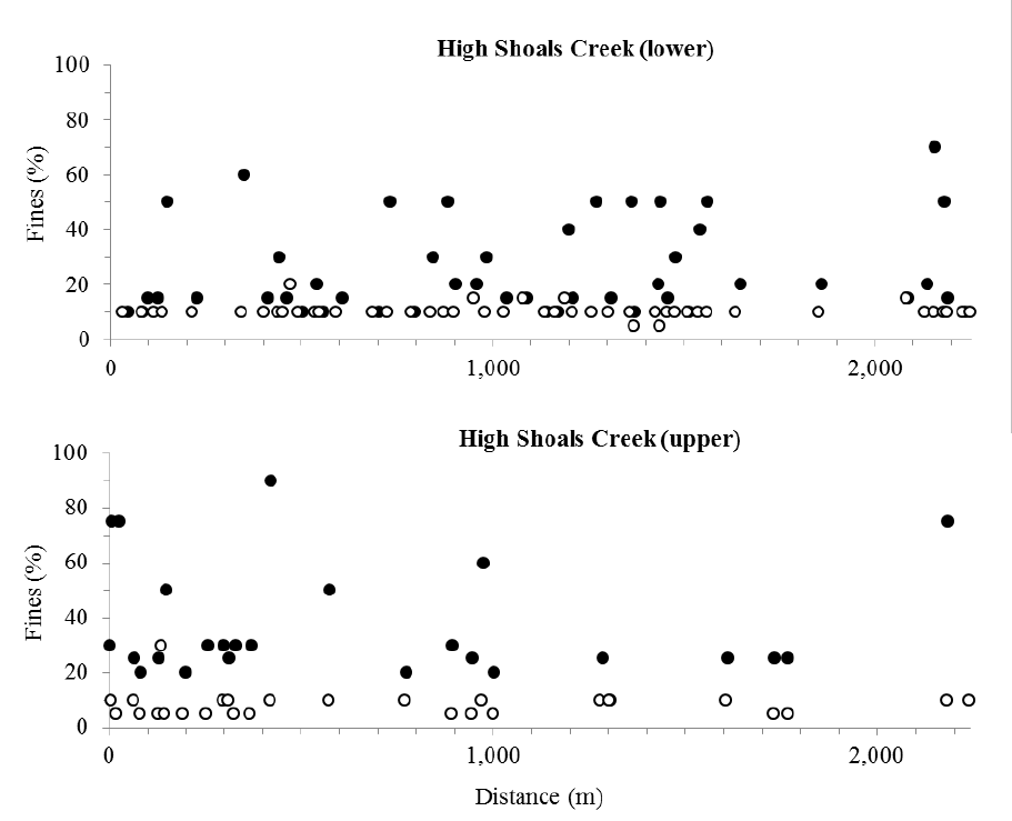
Figure 8. Percent of each pool and riffle channel bottom comprised of fine sediment.............................. 20

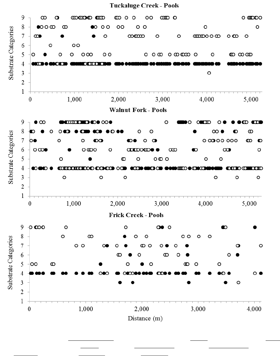
Figure 9. Dominant and subdominant substrate category present in pools ................................................ 25

Figure 10. Dominant and subdominant substrate category present in riffles ............................................. 30

Figure 11. Quantity of large wood per kilometer ....................................................................................... 35

Figure 12. Count of large wood within individual habitat units in each stream inventoried ..................... 36

Figure 13. Hemlock abundance and condition shown longitudinally for each stream inventory .............. 41

List of Tables

Table 1. Summary of streams inventoried on the Chattahoochee National Forest, 2014. ......................... 45

Table 2. GPS coordinates recorded at the downstream (start) and upstream (end) extent of stream habitat

inventories. .................................................................................................................................................. 46

Table 3. Summary of BVET stream habitat attribute averages collected. ................................................. 47

Table 4. Stream area and unit count of pool, glide, riffle, run, and cascade habitat as observed during

BVET habitat inventories. .......................................................................................................................... 48

Table 5. Percent occurrence of dominant and subdominant substrate size categories in pools (includes

glides) and riffles (includes cascades and runs) in each stream inventoried. See appendix A for substrate

size categories. ............................................................................................................................................ 49

Table 6. Large wood (LW) per kilometer observed during BVET habitat inventories. LW size classes:

LW1 = 1-5 m length, 10-55 cm diameter; LW2 = 1-5 m length, >55 cm diameter; LW3 = >5 m length,

10-55 cm diameter; LW4 = >5 m length, >55 cm diameter; RW = rootwad. ............................................. 50

Introduction

Past land management practices including logging and road building, have left trout streams on

the Chattahoochee-Oconee National Forest (CONF), Georgia with a legacy of degraded habitat, including

long shallow riffles, lack of pool habitat, large deposits of sediment in pools, and decreased amounts of

large wood (Waters 1995). Both native (Brook Trout, Salvelinus fontinalis) and naturalized (Brown

Trout, Salmo trutta; Rainbow Trout, Oncorhynchus mykiss) trout populations on the CONF are impacted

by these conditions. If other conditions (water temperature and chemistry, exploitation rates, etc.) remain

the same or improve, the recovery and persistence of the trout resource could be supported by habitat

restoration including the control of excess sediment inputs and the transport and addition of large wood.

Trout populations can be impeded by lack of deep pools, high amounts of fine sediment, and

insufficient large wood to create complex habitat. Wood of all sizes is an important feature of streams

flowing through forested areas. In particular, large wood (LW) and other obstructions such as boulders

slow flow, trap sediments, and damp and delay flood peaks (Montgomery et al. 2003). Tree boles (i.e.

tree trunks or rootwads) are major pool forming elements and wood contributes to aquatic habitat in

diverse ways such as providing cover from predators, refuge from high velocity flow, as well as the LW

being the substrate and organic matter for macroinvertebrates (Benke and Wallace 2003, Dolloff and

Warren 2003). Large wood is considered so beneficial that riparian forests today are managed for LW

inputs (Boyer et al. 2003, Jacobs 2004) and where recruitment or loading is judged insufficient, LW is

intentionally added to stream channels (Reich et al. 2003).

Wood naturally enters stream channels by various avenues including bank undermining or

blowdown of individual trees or groups of trees and transport en masse in debris flows or landslides from

upstream channels or adjacent riparian areas (Swanson 2003). Although logging was one of the more

dramatic causes for the decline in large wood loading, other human influences such as the construction of

roads and trails and land clearing in general have influenced both the rate and amount of large wood

entering streams (Nakamura and Swanson 2003). Invasive species can also lead to variation in the rate of

LW recruitment. Since the beginning of the 20

century a fungus, inadvertently brought to North

America on nursery stock from Asia, has killed nearly all American chestnut (Castenea dentate) trees.

American chestnut was a dominant tree throughout much of the eastern US where, except for areas of

salvage, its demise resulted in higher than expected rates of large wood and large wood recruitment to

streams and riparian areas. Today, hemlock wooly adelgid (Adelges tsugae), an aphid-like insect from

Japan threatens another keystone species of eastern forests, eastern hemlock, with a similar fate. Eastern

hemlock trees in the CONF watersheds are infested by the hemlock wooly adelgid resulting in a rapid

decline of hemlock trees, a major component of streamside vegetation. With seedling hemlock trees

unable to reach maturity in the presence of hemlock wooly adelgid, dead hemlock trees located in the

riparian area are a temporary source of large wood for these streams. Dead or dying hemlocks may be

allowed to recruit to the stream channel through natural processes, or may be intentionally added to the

stream channel.

Large wood additions will encourage pool formation and sediment scour, increasing the amount

of suitable spawning habitat for trout (Ryan et al. 2014, Faustini and Jones 2003, Thompson 1995).

Habitat assessments are needed to optimize the effectiveness of habitat remediation projects. In summer

2014, the CONF partnered with the USDA Forest Service, Southern Research Station, Center for Aquatic

Technology Transfer (CATT) to complete stream habitat inventories in the Blue Ridge District and

Chattooga River District of the CONF (Figure 1). Our goals were to: 1) quantify current stream habitat

conditions; and 2) describe Hemlock abundance and condition within the riparian area. The CATT

deployed a 6-person crew to the CONF from August 7-14, 2014 to inventory stream habitat and describe

hemlock abundance and condition.

Methods

Site Selections and Reach Layout

The streams inventoried, and the inventoried reach extent on each stream, were selected by Mike

Joyce, CONF Forest Fish Biologist.

Habitat Inventory

We performed a basinwide visual estimation technique (BVET) habitat inventory on 11 streams,

two of which were split into a lower and upper section due to different crew members performing the data

observations (Figure 1, Table 1) (Dolloff et al. 1993). The BVET is a two-stage visual estimation

technique to quantify stream habitat. During the first stage, habitat was stratified into similar groups

based on naturally occurring habitat units including pools (areas in the stream with concave bottom

profile, gradient equal to zero, greater than average depth, and smooth water surface), and riffles (areas in

the stream with convex bottom profile, greater than average gradient, less than average depth, and

turbulent water surface). Glides (areas in the stream similar to pools, but with average depth and flat

bottom profile) were identified during the inventory, but were grouped with pools for some data analysis.

Runs (areas in the stream similar to riffles but with average depth, less turbulent flow, and flat bottom

profile) and cascades (areas in the stream with > 12% gradient, high velocity, and exposed bedrock or

boulders) were grouped with riffles for some data analysis.

Habitat in each section of stream was classified and inventoried by a 2 or 3 person crew. One

crew member identified each habitat unit by type (as described above), estimated average wetted width,

average and maximum depth, riffle crest depth (RCD), substrate composition, and percent fines. The

length of each habitat unit was measured with a hip chain. Average wetted width was visually estimated.

Average and maximum depth of each habitat unit were estimated by taking depth measurements at

various places across the channel profile with a graduated staff marked in 5 cm increments. The RCD

was estimated by measuring water depth at the deepest point in the hydraulic control between riffles and

pools. The RCD was subtracted from average pool depth to obtain an estimate of residual pool depth.

Substrates were assigned to one of nine size classes (Appendix A). Dominant substrate (covered greatest

amount of surface area in habitat unit) and subdominant substrate (covered 2

greatest amount of surface

area in habitat unit) were visually estimated. Percent fines is the percent surface area of the stream bed

consisting of sand, silt, or clay substrate particles (particles < 2 mm diameter).

Where encountered, the distance at the upstream end of channel features, as well as additional

attributes described in Appendix A, were recorded for waterfalls, tributaries, side-channels, braids, seeps,

landslides, and ‘other’ miscellaneous features encountered (e.g. campsites, fish habitat structures, etc.). In

addition, a photograph and GPS ID (as well as additional attributes described in Appendix A) were

recorded for waterfalls and crossing features (bridges, fords, dams, and culverts).

The second crew member classified and inventoried large wood (LW) within the bankfull channel

and recorded all data. LW was assigned to one of four size classes (Appendix A). All wood less than 1.0

m long and less than 10 cm in diameter were omitted from the inventory.

The first unit of each habitat type selected for intensive (second stage) sampling (e.g. accurate

measurement of wetted width) was determined randomly. Additional units were selected systematically

(every 10

habitat unit type for streams >1000 m and every 5

habitat unit type for streams <500 m). The

wetted width of each systematically selected habitat unit was measured with a meter tape across at least

three transects and averaged. For the reach between each second stage fast water habitat unit, we

estimated the abundance and condition of Hemlock trees within the riparian area (Appendix A).

The ratio of measured to visually estimated area was used to calibrate all estimates, which

enabled the calculation of total stream area by habitat type (Hankin and Reeves 1988). The BVET

calculations were computed with a Microsoft Excel spreadsheet using formulas found in Dolloff et al.

(1993). Data were summarized using Excel spreadsheets. See Appendix A for detailed field methods.

Results

From August 7-14

2014 we inventoried 11 streams totaling 50.2 km of stream habitat on the

CONF (Figure 1-5, Table 1). GPS coordinates for the start and end location of the inventories, are

available in Table 2.

Depth and Width

Mean residual pool depth (the riffle crest depth was subtracted from average pool depth to obtain

an estimate of residual pool depth which could occur during low flow conditions) ranged from 12 cm to

28 cm among the inventoried streams (Table 3). All streams tended to have somewhat deeper maximum

pool depths in the downstream reaches than in reaches upstream that are higher in the watershed (Figure

6). The average wetted pool width ranged from 1.6 m for Board Camp Creek to 7.2 m for Chester Creek

(lower), followed by 6.5 m for Holcomb Creek (Table 3). The average wetted riffle width ranged from

2.4 m for both Board Camp Creek and Chester Creek (upper) up to 8.6 m for High Shoals (upper),

followed by 6.9 m for Chester Creek (lower) (Table 3).

Habitat Area

Only a few streams had >30% slow water (pools + glides) habitat; Walnut Fork, Holcomb Creek,

and Chester Creek (lower) (Figure 7, Table 4). Fast water (riffle + run + cascade) habitat made up the

majority, being >50% for all streams except Holcomb Creek (Figure 7, Table 4). Fast water habitat

exceeded 90% in Chastain Creek and High Shoals Creek (upper) (Figure 7, Table 4). Though the

majority of the habitat area is fast water habitat (a result of larger unit size), the quantity (i.e. unit count)

of slow water units (pool and glide) to fast water units (riffle, run, cascade) was similar for most streams

(Table 4). Holcomb Creek had the highest percentage of pool (32%), glide (16%), and run (10%) habitat

(Figure 7, Table 4). The cascade habitat area was ≥5% for Tuckaluge Creek, Walnut Fork, Lovinggood

Creek, and Martin Creek (Figure 7, Table 4).

% Fines and Substrate

The average percent fines (percent of habitat unit’s channel bottom covered by sand, silt, or clay)

in pools was high (i.e. ≥35%) in all streams except High Shoals Creek (lower), which had 25% fines

(Table 3). The percent fines in riffles were much lower, never exceeding an average of 20% in any of the

streams (Table 3). Tuckaluge Creek and Lovinggood Creek had the most consistently high percent fines

in pools (Figure 8).

In pools, the dominant substrate was most frequently sand, cobble, and bedrock; the substrate

types small gravel, large gravel, and boulder were also present, but typically as a subdominant substrate

(Table 5, Figure 9). In riffles, the dominant substrate was most frequently large gravel, cobble, boulder,

and bedrock; the substrate types sand and small gravel were also present, but most often as a subdominant

substrate (Table 5, Figure 10). In some streams there are noticeable changes in substrate type with

distance upstream. In Lovinggood Creek riffles, boulder and bedrock substrate transitions to small gravel

and large gravel at ~3,300 m (Figure 10). In Bryant Creek, there is a change from bedrock to gravels at

~3,400 m in both pools and riffles (Figure 9 and 10).

Large Wood

The total pieces of large wood per kilometer (LW/km) ranged from 124 LW/km in High Shoals

Creek (lower) to 245 LW/km in Tuckaluge Creek (Figure 11, Table 6). The majority of LW was in small

diameter size classes (10-55 cm diameter) (Figure 11, Table 6). Bryant Creek had the largest amount (11

LW4/km) of size class 4 (>5 m length, >55 cm diameter) (Figure 11, Table 6). Large wood is distributed

fairly evenly throughout the inventoried reaches; there are occurrences of log jams resulting in higher

wood counts within an individual habitat unit (Figure 12).

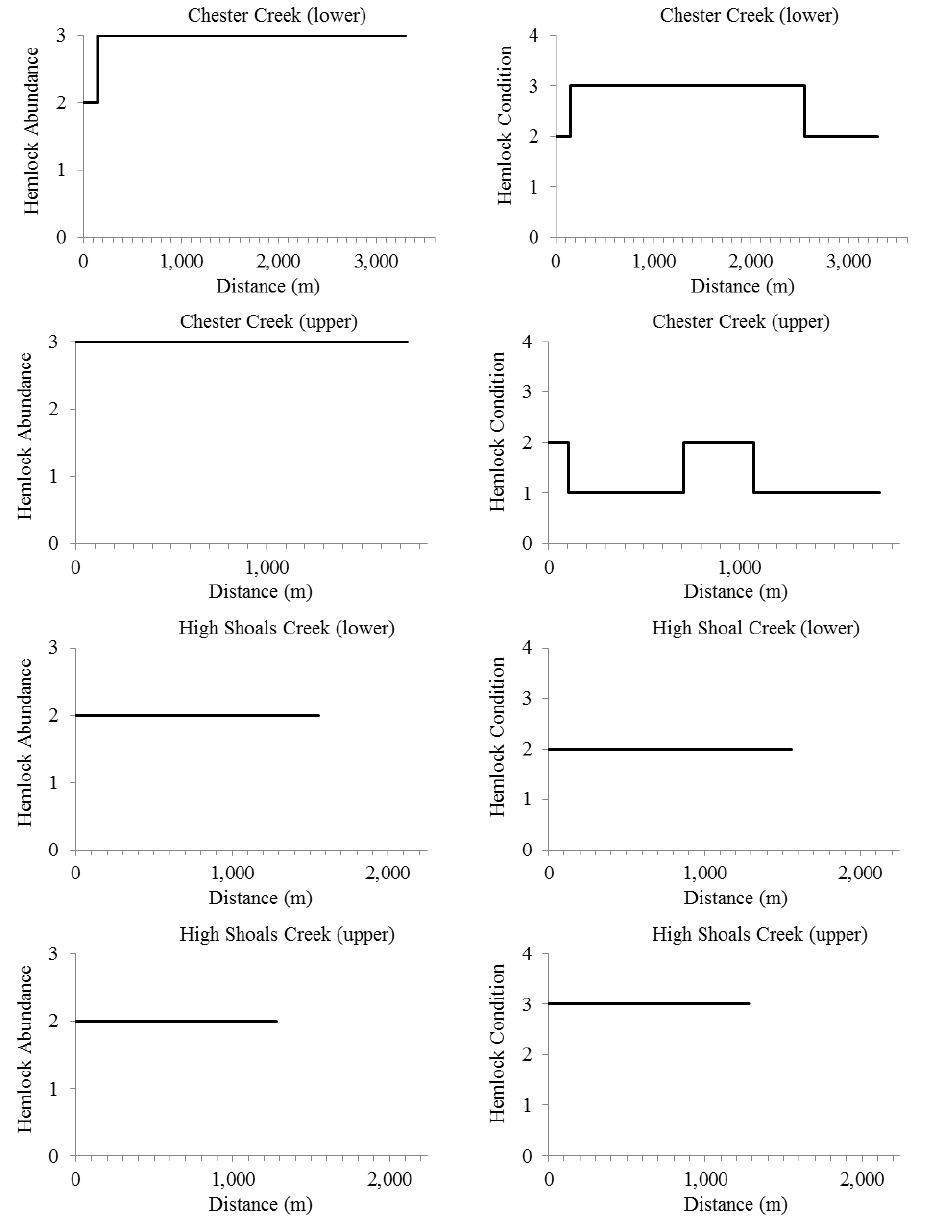
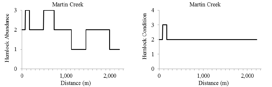
Hemlock Abundance and Condition

Hemlocks were present in the riparian area of all streams and showed varying degrees of

infestation with Hemlock Wooly Adelgid (Figure 13). The following streams had high hemlock

abundance for the majority of the inventoried reach: Tuckaluge Creek, Lovinggood Creek, Holcomb

Creek, and Chester Creek (lower & upper) (Figure 13). The following streams had long reaches where

dead Hemlocks were present: Lovinggood Creek, Chastain Creek, Chester Creek (lower), and High

Shoals Creek (upper) (Figure 13).

Discussion

The inventoried streams are characteristic of those impacted by early 20

century forestry

practices. Many of them have long and shallow riffles, shallow residual pool depths, high percent fines,

and low amounts of LW in the largest size classes. Many also contain log weir fish habitat structures

such as K-dams, installed by the CONF and its partners to mitigate the impacts of those early forestry

practices. While some of these structures are recent additions and others are reaching the end of their

designed lifespan, they were all installed to increase habitat complexity by creating pool habitat and cover

for fish, as well as to trap spawning gravel and flush out fine sediments (Seehorn 1992).

The large-scale loss of hemlocks from hemlock wooly adelgid infestations, though tragic, also

presents a new opportunity as the CONF continues to address the impacts on the Forest from historical

land use. The riparian areas of all the inventoried streams contain hemlock trees infested with hemlock

wooly adelgid. Over time some of these hemlocks will naturally fall into the stream channel, or they can

be manually felled and placed. Many of the inventoried streams have low amounts of LW/km (Walnut

Fork, Frick Creek, Chastain Creek, Board Camp Creek, and High Shoals Creek lower all had <150

LW/km) and all were largely lacking in LW4/km, with the possible exception of Bryant Creek (>10%

LW4). Given the high number of dead or dying hemlocks, these streams are prime targets for LW

treatments.

Sand was prevalent as both a dominant and subdominant substrate in many of the streams, as is

evident by the high percent fines observed in most pools. In addition to large wood improving stream

habitat though pool creation and habitat complexity, newly formed plunge pools could help flush out fine

sediments and expose patches of spawning gravel for trout (Ryan et al. 2014, Faustini and Jones 2003,

Thompson 1995).

Land management practices such as wholesale logging in the watershed in the early 1900’s are

still impacting the number and size of trees available, as well as sediment inputs. Efforts to reverse or

mitigate habitat degradation effects have been ongoing for decades and will continue into the foreseeable

future. Clearly, decisions made by today’s land managers will impact large wood recruitment and

retention, and sediment transport and deposition, for decades to come. New challenges may present new

opportunities and we encourage the CONF and its partners to continue their work to improve stream

habitat.

Data Availability

Summer 2014 stream habitat data reside in a MS Access database, which is managed by the

CATT, and a copy has been provided to Mike Joyce, CONF Forest Fish Biologist. We will work with the

CONF to develop custom queries and reports for the MS Access database, as needed.

Literature Cited

Benke, A. C. and J. B. Wallace. 2003. Influence of wood on invertebrate communities in streams and

rivers. In McMinn, J. W., D. A. Crossley, Jr. Biodiversity and coarse woody debris in southern

forests, proceedings of the workshop on coarse woody debris in southern forests: effects on

biodiversity; 1993 October 18 – 20; Athens, VA. General Technical Report SE-94. Asheville,

NC: U. S. Department of Agriculture, Forest Service, Southern Research Station.

Boyer, K. L., D. R. Berg, and S. V. Gregory. 2003. Riparian management for wood in rivers. Pages 407-

420 in S. V. Gregory, K. L. Boyer, and A. M. Gurnell, editors. The ecology and management of

wood in world rivers. American Fisheries Society, Symposium 37, Bethesda, Maryland.

Dolloff, C. A., D. G. Hankin, and G. H. Reeves. 1993. Basinwide estimation of habitat and fish

populations in streams. General Technical Report SE-83. Asheville, North Carolina: U.S.

Department of Agriculture, Southeastern Forest Experiment Station.

Dolloff, C. A. and M. L. Warren, Jr. 2003. Fish relationships with large wood in small rivers. In Gregory,

S. V., K. L. Boyer, and A. M. Gurnell, editors. The ecology and management of wood in world

rivers. American Fisheries Society, Symposium 37, Bethesda, Maryland.

Faustini, J.M. and J.A. Jones. 2003. Influence of large woody debris on channel morphology and

dynamics in steep, boulder-rich mountain streams, western Cascades, Oregon. Geomorphology

51:187-205.

Jacobs, R. 2004. Revised land and resource monitoring plan, Sumter National Forest. Management

bulletin R8-MB-116A. Atlanta, GA: U. S. Department of Agriculture, Forest Service, Southern

Region.

Montgomery, D. R., B. D. Collins, J. M. Buffington, and T. B. Abbe. 2003. Geomorphic effects of wood

in rivers. In McMinn, J. W., D. A. Crossley, Jr. Biodiversity and coarse woody debris in southern

forests, proceedings of the workshop on coarse woody debris in southern forests: effects on

biodiversity; 1993 October 18 – 20; Athens, VA. General Technical Report SE-94. Asheville,

NC: U. S. Department of Agriculture, Forest Service, Southern Research Station.

Nakamura, F. and F. J. Swanson. 2003. Dynamics of wood in rivers in the context of ecological

disturbance. Pages 279-298 in S. V. Gregory, K. L. Boyer, and A. M. Gurnell, editors. The

ecology and management of wood in world rivers. American Fisheries Society, Symposium 37,

Bethesda, Maryland.

Reich, M., J. L. Kershner, and R. C. Wildman. 2003. Restoring streams with large wood: A synthesis.

Pages 355-365 in S. V. Gregory, K. L. Boyer, and A. M. Gurnell, editors. The ecology and

management of wood in world rivers. American Fisheries Society, Symposium 37, Bethesda,

Maryland.

Ryan, S.E., E.L. Bishop, and J.M. Daniels. 2014. Influence of large wood on channel morphology and

sediment storage in headwater mountain streams, Fraser Experimental Forest, Colorado.

Geomorphology 217:73-88.

Seehorn, M. E. 1992. Stream habitat improvement handbook, Technical Publication R8-TP 16, USDA

Forest Service, Southern Region, 1720 Peachtree Road, N. W., Atlanta, GA.

Swanson, F. J. 2003. Wood in rivers: A landscape perspective. Pages 299-314 in S. V. Gregory, K. L.

Boyer, and A. M. Gurnell, editors. The ecology and management of wood in world rivers.

American Fisheries Society, Symposium 37, Bethesda, Maryland.

Thompson, D.M. 1995. The effects of large organic debris on sediment processes and stream morphology

in Vermont. Geomorphology 11:235-244.

Waters, T. F. 1995. Sediment in streams: sources, biological effects, and control. American Fisheries

Society Monograph 7.

Figure 1. Streams inventoried on the Chattahoochee National Forest, Georgia.

Figure 2. BVET inventory start and end locations on Lovinggood Creek, Chester Creek, and Frick Creek

on the Chattahoochee National Forest, Georgia.

Figure 3. BVET inventory start and end locations on Bryant Creek and Board Camp Creek on the

Chattahoochee National Forest, Georgia.

Figure 4. BVET inventory start and end locations on High Shoals Creek and Chastain Creek on the

Chattahoochee National Forest, Georgia.

Figure 5. BVET inventory start and end locations on Martin Creek, Tuckaluge Creek, Walnut Fork, and

Holcomb Creek on the Chattahoochee National Forest, Georgia.

Figure 6. Maximum pool depth (bars) and residual pool depth (circles) shown longitudinally for each

stream inventory.

Figure 6 continued. Maximum pool depth (bars) and residual pool depth (circles) shown longitudinally

for each stream inventory.

Figure 6 continued. Maximum pool depth (bars) and residual pool depth (circles) shown longitudinally

for each stream inventory.

Figure 6 continued. Maximum pool depth (bars) and residual pool depth (circles) shown longitudinally

for each stream inventory.

Figure 6 continued. Maximum pool depth (bars) and residual pool depth (circles) shown longitudinally

for each stream inventory.

Figure 7. Percent pool, glide, riffle, run, and cascade habitat area.

Figure 8. Percent of each pool (solid circles) and riffle (open circles) channel bottom comprised of fine

sediment (sand, silt, and/or clay).

Figure 8 continued. Percent of each pool (solid circles) and riffle (open circles) channel bottom

comprised of fine sediment (sand, silt, and/or clay).

Figure 8 continued. Percent of each pool (solid circles) and riffle (open circles) channel bottom

comprised of fine sediment (sand, silt, and/or clay).

Figure 8 continued. Percent of each pool (solid circles) and riffle (open circles) channel bottom

comprised of fine sediment (sand, silt, and/or clay).

Figure 8 continued. Percent of each pool (solid circles) and riffle (open circles) channel bottom

comprised of fine sediment (sand, silt, and/or clay).

Figure 9. Dominant (solid circles) and subdominant (open circles) substrate category present in pools.

Substrate size categories: 1 Organic Matter = dead leaves, detritus, etc.; 2 Clay = sticky, holds form; 3 Silt

= slippery, doesn’t hold form; 4 Sand = silt-2 mm; 5 Small Gravel = 3-16 mm; 6 Large Gravel = 17-64

mm; 7 Cobble = 65-256 mm; 8 Boulder = >256 mm; 9 Bedrock = solid rock.

Figure 9 continued. Dominant (solid circles) and subdominant (open circles) substrate category present in

pools. Substrate size categories: 1 Organic Matter = dead leaves, detritus, etc.; 2 Clay = sticky, holds

form; 3 Silt = slippery, doesn’t hold form; 4 Sand = silt-2 mm; 5 Small Gravel = 3-16 mm; 6 Large

Gravel = 17-64 mm; 7 Cobble = 65-256 mm; 8 Boulder = >256 mm; 9 Bedrock = solid rock.

Figure 9 continued. Dominant (solid circles) and subdominant (open circles) substrate category present in

pools. Substrate size categories: 1 Organic Matter = dead leaves, detritus, etc.; 2 Clay = sticky, holds

form; 3 Silt = slippery, doesn’t hold form; 4 Sand = silt-2 mm; 5 Small Gravel = 3-16 mm; 6 Large

Gravel = 17-64 mm; 7 Cobble = 65-256 mm; 8 Boulder = >256 mm; 9 Bedrock = solid rock.

Figure 9 continued. Dominant (solid circles) and subdominant (open circles) substrate category present in

pools. Substrate size categories: 1 Organic Matter = dead leaves, detritus, etc.; 2 Clay = sticky, holds

form; 3 Silt = slippery, doesn’t hold form; 4 Sand = silt-2 mm; 5 Small Gravel = 3-16 mm; 6 Large

Gravel = 17-64 mm; 7 Cobble = 65-256 mm; 8 Boulder = >256 mm; 9 Bedrock = solid rock.

Figure 9 continued. Dominant (solid circles) and subdominant (open circles) substrate category present in

pools. Substrate size categories: 1 Organic Matter = dead leaves, detritus, etc.; 2 Clay = sticky, holds

form; 3 Silt = slippery, doesn’t hold form; 4 Sand = silt-2 mm; 5 Small Gravel = 3-16 mm; 6 Large

Gravel = 17-64 mm; 7 Cobble = 65-256 mm; 8 Boulder = >256 mm; 9 Bedrock = solid rock.

Figure 10. Dominant (solid circles) and subdominant (open circles) substrate category present in riffles.

Substrate size categories: 1 Organic Matter = dead leaves, detritus, etc.; 2 Clay = sticky, holds form; 3 Silt

= slippery, doesn’t hold form; 4 Sand = silt-2 mm; 5 Small Gravel = 3-16 mm; 6 Large Gravel = 17-64

mm; 7 Cobble = 65-256 mm; 8 Boulder = >256 mm; 9 Bedrock = solid rock.

Figure 10 continued. Dominant (solid circles) and subdominant (open circles) substrate category present

in riffles. Substrate size categories: 1 Organic Matter = dead leaves, detritus, etc.; 2 Clay = sticky, holds

form; 3 Silt = slippery, doesn’t hold form; 4 Sand = silt-2 mm; 5 Small Gravel = 3-16 mm; 6 Large

Gravel = 17-64 mm; 7 Cobble = 65-256 mm; 8 Boulder = >256 mm; 9 Bedrock = solid rock.

Figure 10 continued. Dominant (solid circles) and subdominant (open circles) substrate category present

in riffles. Substrate size categories: 1 Organic Matter = dead leaves, detritus, etc.; 2 Clay = sticky, holds

form; 3 Silt = slippery, doesn’t hold form; 4 Sand = silt-2 mm; 5 Small Gravel = 3-16 mm; 6 Large

Gravel = 17-64 mm; 7 Cobble = 65-256 mm; 8 Boulder = >256 mm; 9 Bedrock = solid rock.

Figure 10 continued. Dominant (solid circles) and subdominant (open circles) substrate category present

in riffles. Substrate size categories: 1 Organic Matter = dead leaves, detritus, etc.; 2 Clay = sticky, holds

form; 3 Silt = slippery, doesn’t hold form; 4 Sand = silt-2 mm; 5 Small Gravel = 3-16 mm; 6 Large

Gravel = 17-64 mm; 7 Cobble = 65-256 mm; 8 Boulder = >256 mm; 9 Bedrock = solid rock.

Figure 10 continued. Dominant (solid circles) and subdominant (open circles) substrate category present

in riffles. Substrate size categories: 1 Organic Matter = dead leaves, detritus, etc.; 2 Clay = sticky, holds

form; 3 Silt = slippery, doesn’t hold form; 4 Sand = silt-2 mm; 5 Small Gravel = 3-16 mm; 6 Large

Gravel = 17-64 mm; 7 Cobble = 65-256 mm; 8 Boulder = >256 mm; 9 Bedrock = solid rock.

Figure 11. Quantity of large wood (LW; dead and down, any part within bankfull channel) per kilometer. LW size classes: LW1 = 1-5 m length,

10-55 cm diameter; LW2 = 1-5 m length, >55 cm diameter; LW3 = >5 m length, 10-55 cm diameter; LW4 = >5 m length, >55 cm diameter; RW =

rootwad.

Figure 12. Count of large wood (bars = size classes 1, 2, 3, 4, and rootwad combined; open circles = size

4 only) within individual habitat units in each stream inventoried. Tuckaluge Cr. LW n=1,284 and habitat

unit n=263, Walnut Fk. LW n=759 and habitat unit n=311, and Frick Cr. LW n=614 and habitat unit

n=120.

Figure 12 continued. Count of large wood (bars = size classes 1, 2, 3, 4, and rootwad combined; open

circles = size 4 only) within individual habitat units in each stream inventoried. Lovinggood Cr. LW

n=1,272 and habitat unit n=346, Chastain Cr. LW n=147 and habitat unit n=24, and Holcomb Cr. LW

n=1,569 and habitat unit n=342.

Figure 12 continued. Count of large wood (bars = size classes 1, 2, 3, 4, and rootwad combined; open

circles = size 4 only) within individual habitat units in each stream inventoried. Bryant Cr. LW n=1,078

and habitat unit n=350, Board Camp Cr. LW n=266 and habitat unit n=96, and Martin Cr. LW n=428 and

habitat unit n=145.

Figure 12 continued. Count of large wood (bars = size classes 1, 2, 3, 4, and rootwad combined; open

circles = size 4 only) within individual habitat units in each stream inventoried. Chester Cr. (lower) LW

n=568 and habitat unit n=150, and Chester Cr. (upper) LW n=347 and habitat unit n=72.

Figure 12 continued. Count of large wood (bars = size classes 1, 2, 3, 4, and rootwad combined; open

circles = size 4 only) within individual habitat units in each stream inventoried. High Sholas Cr. (lower)

LW n=279 and habitat unit n=95, and High Shoals Cr. (upper) LW n=489 and habitat unit n=53.

Figure 13. Hemlock abundance (0 = none; 1 = 1-10; 2 = 11-50, 3 = >50) and condition (0 = Healthy, 1 =

Early Infestation, 2 = Late Infestation, 3 = Mortality, 4 = LW Recruiting) shown longitudinally for each

stream inventory (see appendix A for detailed categories).

Figure 13 continued. Hemlock abundance (0 = none; 1 = 1-10; 2 = 11-50, 3 = >50) and condition (0 =

Healthy, 1 = Early Infestation, 2 = Late Infestation, 3 = Mortality, 4 = LW Recruiting) shown

longitudinally for each stream inventory (see appendix A for detailed categories).

Figure 13 continued. Hemlock abundance (0 = none; 1 = 1-10; 2 = 11-50, 3 = >50) and condition (0 =

Healthy, 1 = Early Infestation, 2 = Late Infestation, 3 = Mortality, 4 = LW Recruiting) shown

longitudinally for each stream inventory (see appendix A for detailed categories).

Figure 13 continued. Hemlock abundance (0 = none; 1 = 1-10; 2 = 11-50, 3 = >50) and condition (0 =

Healthy, 1 = Early Infestation, 2 = Late Infestation, 3 = Mortality, 4 = LW Recruiting) shown

longitudinally for each stream inventory (see appendix A for detailed categories).

Table 1. Summary of streams inventoried on the Chattahoochee National Forest, 2014.

BVET

Site # Stream Name Topo Quad Start End habitat (km) Start Location

2014-01 Tuckaluge Creek Rabun Bald 8/7/14 8/9/14 5.2 FS boundary

2014-02 Walnut Fork Rabun Bald 8/8/14 8/10/14 5.3 FS boundary

2014-03 Frick Creek Noontootla 8/11/14 8/12/14 4.1 Chester Creek confluence

2014-04 Lovinggood Creek Noontootla 8/11/14 8/12/14 5.3 Noontootla Creek confluence

2014-05 Chastain Creek Macedonia 8/10/14 8/10/14 1.0 Jakes Branch confluence

2014-06 Holcomb Creek Satolah, Rabun Bald 8/8/14 8/10/14 9.3 Top of gorge 250 m upstream of 3 Forks

2014-07 Bryant Creek Mulky Gap 8/11/14 8/12/14 5.5 Cooper Creek confluence

2014-08 Board Camp Creek Coosa Bald 8/13/14 8/13/14 2.0 Logan Creek confluence

2014-09L Chester Creek (lower) Noontootla 8/13/14 8/14/14 3.6 Noontootla Creek confluence

2014-09U Chester Creek (upper) Noontootla 8/13/14 8/13/14 1.8 Davis Creek confluence

2014-10L High Shoals Creek (lower) Tray Mountain 8/14/14 8/14/14 2.3 750 m upstream of FS boundary

2014-10U High Shoals Creek (upper) Tray Mountain 8/14/14 8/14/14 2.4 1st trib on left, upstream of Maple Spring Br.

2014-13 Martin Creek Rabun Bald 8/8/14 8/8/14 2.3 Rock Mountain Creek confluence

Total 50.2

Date

Table 2. GPS coordinates recorded at the downstream (start) and upstream (end) extent of stream habitat inventories.

Site # Stream Name Downstream Inventory Start Upstream Inventory End

2014-01 Tuckaluge Creek N34.89987 W83.29929 N34.92660 W83.33071

2014-02 Walnut Fork N34.90861 W83.27467 N34.94530 W83.29630

2014-03 Frick Creek N34.66033 W84.17898 N34.65480 W84.14505

2014-04 Lovinggood Creek N34.69545 W84.21598 N34.66487 W84.21951

2014-05 Chastain Creek N34.87409 W83.62648 N34.87915 W83.63451

2014-06 Holcomb Creek N34.96630 W83.21609 N34.98224 W83.29099

2014-07 Bryant Creek N34.75498 W84.04173 N34.78210 W84.01450

2014-08 Board Camp Creek N34.76522 W83.99317 N34.76630 W83.97594

2014-09L Chester Creek (lower) N34.67238 W84.19704 N34.65422 W84.17827

2014-09U Chester Creek (upper) N34.65422 W84.17827 N34.64201 W84.17008

2014-10L High Shoals Creek (lower) N34.81719 W83.72419 N34.79956 W83.71537

2014-10U High Shoals Creek (upper) N34.79969 W83.71526 N34.80080 W83.69744

2014-13 Martin Creek N34.89125 W83.34288 N34.90201 W83.35909

GPS (NAD83)

Table 3. Summary of BVET stream habitat attribute averages collected.

*Residual pool depth = average pool depth – riffle crest depth

Pools Riffles Pools Riffles Pools Riffles Pools Riffles

2014-01 Tuckaluge Creek 40 15 63 34 28 4.8 4.2 74 20

2014-02 Walnut Fork 38 17 55 29 26 3.7 3.7 44 16

2014-03 Frick Creek 32 17 52 40 17 3.5 3.6 58 18

2014-04 Lovinggood Creek 35 21 54 35 16 4.2 3.8 60 20

2014-05 Chastain Creek 28 18 43 36 12 3.7 3.5 57 17

2014-06 Holcomb Creek 50 29 77 50 28 6.5 5.7 48 20

2014-07 Bryant Creek 34 17 44 27 20 3.7 4.3 40 14

2014-08 Board Camp Creek 30 14 39 23 20 1.6 2.4 35 12

2014-09L Chester Creek (lower) 47 28 67 49 22 7.2 6.9 44 14

2014-09U Chester Creek (upper) 28 11 43 28 20 3.5 2.4 51 13

2014-10L High Shoals Creek (lower) 37 17 47 29 23 4.1 3.9 25 10

2014-10U High Shoals Creek (upper) 28 10 42 26 20 2.6 8.6 36 8

2014-13 Martin Creek 32 17 43 30 17 3.2 3.8 49 12

Avg. %

Fines

Avg. Wetted

Width (m)

Site #

Stream Name

Mean Avg.

Depth (cm)

Mean Max.

Depth (cm)

Mean Residual

Pool Depth

(cm)*

Table 4. Stream area and unit count of pool, glide, riffle, run, and cascade habitat as observed during BVET habitat inventories.

Site # Stream Name Pool Glide Riffle Run

Cas-

cade

Total Pool Glide Riffle Run

Cas-

cade

Pool Glide Riffle Run

Cas-

cade

2014-01 Tuckaluge Creek 5,465 540 14,289 1,462 1,173 22,929 24% 2% 62% 6% 5% 121 9 103 16 14

2014-02 Walnut Fork 4,010 2,537 13,287 348 1,088 21,269 19% 12% 62% 2% 5% 116 42 128 8 17

2014-03 Frick Creek 1,310 128 12,290 364 327 14,418 9% 1% 85% 3% 2% 55 4 54 5 2

2014-04 Lovinggood Creek 4,823 1,343 13,540 0 1,266 20,973 23% 6% 65% 0% 6% 146 36 150 0 14

2014-05 Chastain Creek 240 49 2,978 33 0 3,300 7% 1% 90% 1% 0% 8 3 12 1 0

2014-06 Holcomb Creek 19,238 9,770 22,989 6,064 1,990 60,052 32% 16% 38% 10% 3% 116 58 119 28 21

2014-07 Bryant Creek 3,911 1,605 15,962 364 420 22,261 18% 7% 72% 2% 2% 120 49 168 11 2

2014-08 Board Camp Creek 449 80 3,594 0 106 4,230 11% 2% 85% 0% 2% 41 7 47 0 1

2014-09L Chester Creek (lower) 6,158 2,261 17,038 0 459 25,915 24% 9% 66% 0% 2% 57 24 64 0 5

2014-09U Chester Creek (upper) 598 261 3,604 21 0 4,484 13% 6% 80% 0% 0% 33 5 33 1 0

2014-10L High Shoals Cr. (lower) 1,531 185 7,485 35 0 9,236 17% 2% 81% 0% 0% 43 4 47 1 0

2014-10U High Shoals Cr. (upper) 256 9 19,425 36 0 19,727 1% 0% 98% 0% 0% 25 1 26 1 0

2014-13 Martin Creek 751 699 5,937 390 442 8,219 9% 9% 72% 5% 5% 30 29 67 13 6

Habitat Area (m

)

Percent Area

Unit Count

Table 5. Percent occurrence of dominant and subdominant substrate size categories in pools (includes glides) and riffles (includes cascades and

runs) in each stream inventoried. See appendix A for substrate size categories.

Organic M.

Clay

Silt

Sand

Small G.

Large G.

Cobble

Boulder

Bedrock

Organic M.

Clay

Silt

Sand

Small G.

Large G.

Cobble

Boulder

Bedrock

Tuckaluge Creek 0% 0% 0% 89% 1% 0% 2% 2% 6% 0% 0% 0% 3% 0% 12% 38% 20% 27%

Walnut Fork 0% 0% 0% 49% 1% 6% 5% 11% 27% 0% 0% 0% 3% 1% 13% 15% 29% 39%

Frick Creek 0% 0% 7% 64% 3% 5% 8% 2% 10% 0% 0% 0% 7% 16% 23% 31% 3% 20%

Lovinggood Creek 0% 0% 0% 69% 4% 1% 8% 8% 10% 0% 0% 0% 0% 5% 19% 36% 26% 15%

Chastain Creek 0% 0% 27% 27% 18% 9% 18% 0% 0% 0% 0% 0% 0% 8% 0% 85% 8% 0%

Holcomb Creek 0% 0% 0% 48% 2% 2% 9% 10% 29% 0% 0% 0% 8% 4% 5% 15% 31% 37%

Bryant Creek 0% 0% 0% 37% 1% 6% 20% 5% 31% 0% 0% 0% 2% 2% 14% 43% 7% 32%

Board Camp Creek 0% 0% 0% 19% 0% 0% 48% 4% 29% 0% 0% 0% 2% 0% 0% 73% 6% 19%

Chester Creek (lower) 0% 0% 0% 44% 0% 1% 9% 19% 27% 0% 0% 0% 0% 0% 6% 16% 39% 39%

Chester Creek (upper) 0% 0% 0% 55% 0% 0% 11% 3% 32% 0% 0% 0% 6% 9% 21% 26% 0% 38%

High Shoals Creek (lower) 0% 0% 0% 4% 0% 0% 64% 17% 15% 0% 0% 0% 0% 0% 0% 96% 4% 0%

High Shoals Creek (upper) 0% 0% 0% 27% 8% 15% 19% 8% 23% 0% 0% 0% 0% 0% 22% 63% 7% 7%

Martin Creek 0% 0% 0% 53% 3% 7% 12% 8% 17% 0% 0% 0% 1% 4% 11% 45% 19% 21%

Tuckaluge Creek 0% 0% 1% 10% 22% 2% 21% 12% 32% 0% 0% 0% 18% 3% 23% 26% 23% 8%

Walnut Fork 0% 0% 4% 35% 6% 15% 13% 12% 15% 0% 0% 3% 32% 5% 18% 29% 9% 4%

Frick Creek 0% 0% 2% 17% 19% 12% 19% 15% 17% 0% 0% 2% 21% 38% 15% 15% 5% 5%

Lovinggood Creek 0% 0% 5% 19% 9% 13% 13% 31% 10% 0% 0% 0% 11% 8% 20% 31% 25% 4%

Chastain Creek 9% 0% 0% 45% 18% 0% 18% 0% 9% 0% 0% 0% 15% 54% 23% 8% 0% 0%

Holcomb Creek 0% 0% 1% 29% 15% 9% 10% 21% 15% 0% 0% 0% 12% 9% 16% 22% 31% 10%

Bryant Creek 0% 0% 1% 38% 12% 15% 18% 7% 9% 0% 0% 0% 18% 11% 30% 18% 22% 1%

Board Camp Creek 0% 0% 4% 50% 2% 23% 15% 6% 0% 0% 0% 0% 6% 0% 71% 13% 10% 0%

Chester Creek (lower) 0% 0% 0% 36% 2% 10% 14% 19% 20% 0% 0% 0% 16% 1% 3% 35% 35% 10%

Chester Creek (upper) 0% 0% 3% 34% 13% 8% 13% 18% 11% 0% 0% 0% 29% 6% 21% 32% 6% 6%

High Shoals Creek (lower) 0% 0% 2% 28% 2% 23% 21% 17% 6% 0% 0% 0% 0% 0% 83% 4% 10% 2%

High Shoals Creek (upper) 0% 0% 0% 38% 27% 8% 15% 8% 4% 0% 0% 0% 7% 0% 41% 33% 11% 7%

Martin Creek 2% 0% 0% 25% 10% 8% 25% 14% 15% 1% 0% 2% 11% 4% 26% 26% 22% 8%

Pool Dominant Substrate

Riffle Dominant Substrate

Pool Subdominant Substrate

Riffle Subdominant Substrate

Table 6. Large wood (LW) per kilometer observed during BVET habitat inventories. LW size classes: LW1 = 1-5 m length, 10-55 cm diameter;

LW2 = 1-5 m length, >55 cm diameter; LW3 = >5 m length, 10-55 cm diameter; LW4 = >5 m length, >55 cm diameter; RW = rootwad.

Site # Stream Name

LW1/

LW2/

LW3/

LW4/

RW/

Total

LW/km

LW1

LW2

LW3

LW4

Total

LW n

2014-01 Tuckaluge Creek 113 2 121 3 6 245 593 10 637 14 30 1,284 5.2

2014-02 Walnut Fork 106 0 31 6 0 144 561 0 165 32 1 759 5.3

2014-03 Frick Creek 80 1 62 3 2 149 329 5 257 13 10 614 4.1

2014-04 Lovinggood Creek 123 0 113 3 1 240 650 1 601 15 5 1,272 5.3

2014-05 Chastain Creek 73 0 65 1 2 141 76 0 68 1 2 147 1.0

2014-06 Holcomb Creek 79 1 84 3 4 170 727 9 774 26 33 1,569 9.3

2014-07 Bryant Creek 112 4 68 11 1 196 619 20 373 60 6 1,078 5.5

2014-08 Board Camp Creek 76 4 50 5 1 136 149 8 99 9 1 266 2.0

2014-09L Chester Creek (lower) 76 0 76 2 3 158 275 0 275 8 10 568 3.6

2014-09U Chester Creek (upper) 100 1 84 2 2 188 184 1 155 3 4 347 1.8

2014-10L High Shoals Creek (lower) 56 0 61 4 2 124 126 1 138 9 5 279 2.3

2014-10U High Shoals Creek (upper) 112 0 85 2 1 200 273 1 208 4 3 489 2.4

2014-13 Martin Creek 135 1 37 7 3 184 313 3 87 17 8 428 2.3

Large Wood per Km

Large Wood Count in Sample Reach

Inventory

Distance

(km)

Appendix A: Field Methods for Stream Habitat Inventory

Guide to Stream Habitat Characterization using the BVET Methodology

in the Chattahoochee National Forest, GA

Prepared by:

United States Department of Agriculture Forest Service

Southern Research Station

Center for Aquatic Technology Transfer (CATT)

1710 Research Center Dr.

Blacksburg, VA 24060-6349

C. Andrew Dolloff, Team Leader

July 2014

Introduction ............................................................................................................................................... 54

References cited in this manual: .............................................................................................................. 55

Outline of BVET Habitat Inventory........................................................................................................ 56

Section 1: Getting Started ........................................................................................................................ 57

Equipment List ......................................................................................................................... 57

Duties ....................................................................................................................................... 57

Header Information .................................................................................................................. 58

Starting the Inventory .............................................................................................................. 58

Section 2: Stream Attributes .................................................................................................................... 59

Unit Type (see abbreviations) .................................................................................................. 59

Unit Number (#) ....................................................................................................................... 60

Distance (m) ............................................................................................................................. 61

Estimated Width (m) ................................................................................................................ 61

Maximum and Average Depth (cm) ........................................................................................ 62

Riffle Crest Depth (cm) ........................................................................................................... 62

Dominant and Subdominant Substrate (1-9) ............................................................................ 63

Percent Fines (%) ..................................................................................................................... 64

Large Wood (1-4 and rootwad) ................................................................................................ 64

Actual Width (m) ..................................................................................................................... 65

Hemlock Condition (0 - 4) ....................................................................................................... 65

Hemlock Abundance (0 - 3) ..................................................................................................... 65

Photo (ID#) .............................................................................................................................. 66

GPS (ID) .................................................................................................................................. 66

Features .................................................................................................................................... 67

Section 3: Wrapping Up ........................................................................................................................... 68

Section 4: Summary .................................................................................................................................. 69

Section 5: GPS Instructions ..................................................................................................................... 70

How to Find a Waypoint on GPS: ........................................................................................... 70

Changing Waypoints:............................................................................................................... 70

Garmin GPS Oregon 400T Cheatsheet .................................................................................... 71

Appendix: Field Guide, Equipment Checklist ....................................................................................... 72

Equipment Checklist ................................................................................................................ 74

Introduction

The Basinwide Visual Estimation Technique (BVET) is a versatile tool used to assess streamwide habitat

conditions in wadeable size streams and rivers. A crew of two individuals performs the inventory using

two-stage visual estimation techniques described in Hankin and Reeves (1988) and Dolloff et al. (1993).

In its most basic form the BVET combines visual estimates with actual measurements to provide a

calibrated estimate of stream area with confidence intervals, however the crew may inventory any number

of other habitat attributes as they walk the length of the stream. Experienced crews can inventory an

average of 2-3 km per day, but this will vary depending on stream size and the number of stream

attributes inventoried.

Before a crew begins a BVET inventory they must receive adequate training, both in the classroom and in

the field. Estimating and measuring a large number of habitat attributes can confuse and overwhelm an

inexperienced crew. Individuals must have an understanding of the basic concepts behind the BVET and

be familiar with habitat attributes before they can effectively and efficiently perform an inventory.

This document was developed to serve as a guide for classroom and field instructions specific to the

Chattahoochee National Forest BVET habitat inventory and to provide a post-training reference for field

crews. It includes an overview of the BVET inventory, defines habitat attributes, instructs how and when

to measure attributes, and provides reference sheets for use in the field. Each trainee should receive a

copy of this manual and is encouraged to take notes in the spaces provided.

References cited in this manual:

Armantrout, N. B., compiler. 1998. Glossary of aquatic habitat inventory terminology. American

Fisheries Society, Bethesda, Maryland.

Bunte, K., and S. R. Abt. 2001. Sampling surface and subsurface particle-size distributions in wadable

gravel- and cobble-bed streams for analyses in sediment transport, hydraulics, and streambed

monitoring. General Technical Report RMRS-GTR-74. Fort Collins, Colorado: U.S. Department

of Agriculture, Forest Service, Rocky Mountain Research Station.

Dolloff, C. A., D. G. Hankin, and G. H. Reeves. 1993. Basinwide estimation of habitat and fish

populations in streams. General Technical Report SE-83. Asheville, North Carolina: U.S.

Department of Agriculture, Southeastern Forest Experimental Station.

Hankin, D. G., and G. H. Reeves. 1988. Estimating total fish abundance and total habitat area in small

streams based on visual estimation methods. Canadian Journal of Fisheries and Aquatic Sciences

45:834-844.

Rosgen, D.L. 1996. Applied River Morphology. Wildland Hydrology Books, Pagosa Springs, Colorado.

Rosgen, D.L., and L. Silvey. 1998 Field Guide for Stream Classification, Wildland Hydrology Books,

Pagosa Springs, Colorado.

Outline of BVET Habitat Inventory

1. Enter ‘Header’ information on the data sheet: --- ‘Header’ information includes date, stream, start

location, crew, etc. and is vitally important to record for future reference.

2. Enter downstream of the starting point, then move upstream and begin the inventory. Tie off the

hipchain, proceed upstream to the starting point, reset the hipchain to zero, and proceed upstream

estimating parameters and recording data in every habitat unit.

3. At the paired sample units perform visual estimates, and then perform measurements. Pair a

minimum of 3 fast and 3 slow-water units; pair more if possible. Typically inventories longer

than 1 km can pair every 10

fast and slow water habitat unit; inventories shorter than 1 km pair

every 5

4. Progress upstream estimating attributes for every unit until the next paired sample unit is reached,

then repeat step 3.

The crew should also take care to record roads, trails, tributaries, dams, waterfalls, road crossing types,

riparian features (wildlife openings, trails, campsites, roads, timber harvest, etc.), and other pertinent

stream features as they progress upstream. Be sure to record hipchain distances when noting such

features. Some features may also require a picture number to be associated with them.

The following sections describe the BVET habitat inventory in detail:

Section 1: Getting Started – equipment, header info, random numbers, starting the inventory

Section 2: Habitat Attributes – definitions, how to estimate or measure, when to record

Section 3: Wrapping Up – what to do when the inventory is completed

Section 4: Summary

Section 5: GPS Instructions

Appendix: field guide, random number tables, equipment checklist

Section 1: Getting Started

Equipment List

 Hipchain

 Camera

 Extra string for hipchain

 Backpack

 Wading rod

 Pencils

 50 m tape measure

 Flagging

 Clinometer

 Markers

 iPad

 Waterproof backup datasheets

 Thermometer

 Clipboard

 Handheld GPS unit

 BVET field guide on waterproof paper

 Topographic maps

 Non-slip wading boots or waders

 Cell Phone

 Water

 First Aid Kit

 Water Filter

 Rain Gear (optional)

 Toilet Paper

The BVET crew consists of two individuals, the ‘observer’ and the ‘recorder’. The observer wears the

hipchain and carries the wading rod. The recorder wears the data logger and carries other equipment in

the backpack. The duties of each individual are listed below.

Duties

Observer

Recorder

Designate habitat units

Track location on quad map

Measure distance

Record data

Estimate width

Determine paired sample location

Estimate depths

Classify and count Large Wood (LW)

Classify substrates

Photo-documentation

Locate features

Document features

Estimate percent fines

GPS-documentation

Both crew members are needed to measure actual widths at designated units. Although the crew has

assigned duties, they should not hesitate to consult with each other if they have questions or feel that a

mistake may have been made. Working as a team will provide the best possible results.

Header Information

Header information is vitally important for future reference. Take the time to record all categories

completely and accurately.

Stream Name

Full name of stream

District

National Forest District name

Quad

USGS 1:24,000 quadrangle name

Date

Record date(s) of inventory

Recorder

Full name of recorder

Observer

Full name of observer

GPS

Record at start and end locations, always use NAD83, Decimal degrees

Location

Detailed written description of start point, include landmarks, road #, etc.

Comments

Record signs of activity in area, water conditions, other pertinent information

Starting the Inventory

After the crew has organized their gear, determined their measurement interval, selected a random

number, and recorded all the header information they are ready to begin the habitat inventory.

The observer should enter the stream slightly downstream of the starting point, tie off the hipchain,

progress upstream to the starting point, reset the hipchain to zero and begin walking upstream through the

first habitat unit. As the observer moves upstream they use the wading rod to measure depth at several

locations in the habitat unit and make observations of unit type, width, substrates, and percent fines.

When they reach the upstream end of the habitat unit they stop, turn to face the unit and report the unit

type, maximum and average depth, riffle crest depth (where appropriate), dominant and subdominant

substrate classes, percent fines, estimated width, and hipchain distance to the recorder.

As the observer moves upstream through the unit, the recorder follows behind, recording the amount of

LW in the habitat unit. The recorder also assigns a number to the habitat unit. The recorder tells the

observer if a unit is designated for measurements (i.e. if it is a ‘paired sample’ unit) only after they have

recorded visual estimates.

The crew continues upstream making estimates in every habitat unit and making estimates and

measurements in every paired sample unit until the inventory endpoint is reached.

Definitions of habitat attributes, how to measure and when to record them, and what to do when the

inventory is complete are covered in the following sections.

Section 2: Stream Attributes

Unit Type (see abbreviations)

Unit Type

Abbreviation

Definition

Riffle

Fast water, turbulent, gradient <12%; shallow reaches characterized

by water flowing over or around rough bed materials that break the

surface during low flows; also include rapids (turbulent with

intermittent whitewater, breaking waves, and exposed boulders),

chutes (rapidly flowing water within narrow, steep slots of bedrock),

and sheets (shallow water flowing over bedrock) if gradient <12%

Cascade

Fast water, turbulent, gradient >12%; highly turbulent series of

short falls and small scour basins, with very rapid water movement;

also include sheets (shallow water flowing over bedrock) and chutes

(rapidly flowing water within narrow, steep slots of bedrock) if

gradient >12%

Run

Fast water, non-turbulent, gradient <12%; deeper than riffles with

little or no surface agitation or flow obstructions and a flat bottom

profile

Pool

Slow water, surface turbulence may or may not be present, gradient

<1%; generally deeper and wider than habitat immediately upstream

and downstream, concave bottom profile; includes dammed pools,

scour pools, and plunge pools

Glide

Slow water, no surface turbulence, gradient <1%; shallow with

little to no flow and flat bottom profile

Underground

UNGR

Stream channel is dry or not containing enough water to form

distinguishable habitat units

*modified from Armantrout (1998)

How to estimate:

Habitat units are separated by ‘breaks’. Breaks can be obvious physical barriers, such as a debris dam

separating two pools or a small waterfall separating a pool and riffle, or may be less obvious transitional

areas. Questions often arise as to whether a break is substantial enough to split two habitat units and

where the exact location of the break occurs. When in doubt, the observer should consult with the

recorder and the team should ‘think like a fish’. To determine if a break should be made, consider

whether a fish would have to make an effort to move across the break and into the next habitat unit. If

not, then it is probably a single habitat unit.

The channel may have both pool and riffle type habitat in the same cross-sectional area. Determine the

predominate habitat type and record it as the unit type. For example if an area contains both pool and

riffle, but the majority of the flow is into and out of the pool habitat, then call the unit a pool.

Questions also often arise as to the minimum size of individual habitat units. Generally, if a habitat unit

is not at least as long as the wetted channel is wide, then do not count it as a separate habitat unit. This

rule may need to be adjusted for streams wider than 5 m. Use best professional judgment in such cases.

See the section 2.1 for a list of features that should also be recorded while performing the inventory.

When to record: every habitat unit

Unit Number (#)

Definition:

Count of habitat units of similar types, used to determine location of paired sample units

How to estimate:

When counting habitat units, group pools and glides (slow water) together, and group riffles, runs, and

cascades (fast water) together. For example, consider the following sequence of habitat units:

Pool – Riffle – Pool – Pool – Riffle - Cascade – Riffle - Glide – Riffle – Pool – Run – Pool – Riffle

Habitat units in this sequence would be counted in the following manner (similar types are shaded same

color):

Unit Type

Unit Number

In the above example, the crew has counted six slow water (pool/glide) units and seven fast water

(riffle/run/cascade) units.

When to record: every habitat unit; not recorded for features

Distance (m)

Definition:

Number of meters (rounded to the whole meter) from the start of the inventory to the upstream end of the

habitat unit or distance from the start of the inventory to upstream end of a feature, used as spatial

reference for data analysis and to locate features in the future.

How to estimate:

The observer walks upstream in the middle of the stream channel with a hipchain measuring device.

When they reach the upstream break between habitat units or the upstream end of a feature they stop and

report the distance to the recorder.

Care should be taken to keep the hipchain string in the middle of the stream, especially around bends and

meanders. If the hipchain should break, retreat to the location where the break occurred, tie off the

hipchain, and continue. If the hipchain is reset for any reason be sure to note it in the comments.

When to record: every habitat unit and feature

Estimated Width (m)

Definition:

Average wetted width of the habitat unit as estimated visually (typically to half-meter accuracy), used to

calculate stream area. Wetted width is the distance from the edge of the water on one side of the main

channel to the edge of the water on the opposite side of the main channel.

How to estimate:

The observer notes the general shape and width of the unit while walking to the upstream end. When they

reach the upstream end of the unit the observer stops, turns to face the unit, and estimates the average

wetted width. Measure the wetted width of the stream before starting each day to calibrate yourself.

When to record: every habitat unit

Maximum and Average Depth (cm)

Definitions:

Maximum Depth – vertical distance from substrate to water surface at deepest point in habitat unit

Average Depth – average vertical distance from substrate to water surface in habitat unit

How to estimate:

The observer uses a wading rod marked in 5 cm increments to measure water depth as they walk upstream

through the habitat unit. Water depth in deepest spot is recorded as the maximum depth. Average depth

is the average of several depth measurements taken throughout the habitat unit.

When to record: every habitat unit

Riffle Crest Depth (cm)

Definition:

Vertical distance from the substrate to the water surface at the deepest point in the riffle crest. The riffle

crest is the shallowest continuous line (usually not straight) across the channel where the water surface

becomes continuously riffled in the transition area between a riffle (or a run or cascade) and a pool (or

glide) (Armantrout 1998); think of it as the last place water would flow out of the pool if the riffle ran dry.

How to estimate:

When the observer reaches the upstream end of a riffle (or a run or cascade) leading into a pool (or glide),

they use the wading rod to measure the deepest point in the riffle crest. Record the depth in the RCD

column for the riffle habitat row.

When to record: at the upstream end of any riffle, run, or cascade leading into a pool or glide

Dominant and Subdominant Substrate (1-9)

Definitions:

Dominant Substrate – size class of stream bed material that covers the greatest amount of surface area

within the wetted channel of the habitat unit.

Subdominant Substrate – size class of stream bed material that covers the 2

greatest amount of surface

area within the wetted channel of the habitat unit.

How to estimate:

The following size classes are used to categorize substrates*. The substrate ‘Number’ is entered into the

dominant and subdominant substrate columns on the datasheet.

Type

Number

Size (mm)

Description

Organic Matter

dead leaves, detritus, etc. – not live plants

Clay

sticky, holds form when rolled into a ball

Silt

slippery, does not hold form when rolled into a ball

Sand

silt – 2

grainy, does not hold form when rolled into ball

Small Gravel

3-16

sand to thumbnail

Large Gravel

17-64

thumbnail to fist

Cobble

65-256

fist to head

Boulder

>256

larger than head

Bedrock

solid rock, parent material, may extend into bank

* these size classes are based on the modified Wentworth scale

As the observer walks through the unit they scan the substrate. When they reach the upstream end of the

unit they stop, turn to face the unit, and determine the dominant and subdominant substrate classes.

Estimate substrate size along the intermediate axis (b-axis). The b-axis is not the longest or shortest axis,

but the intermediate length axis (see below). It is the axis that determines what size sieve the particle

could pass through. Remember that your eyes are naturally drawn to larger size substrates. Be careful

not to bias your estimate by focusing on the large size substrate.

Some units will contain a mixture of particle sizes. Consult with the recorder and use your best

professional judgment to choose the dominant and subdominant sizes.

In units where the substrate is covered in moss, algae, or

macrophytes classify the underlying substrate and make note of the

plant growth in the comments. Only call organic substrate where

there is dead and down leaves or other detritus covering the bottom

of the unit.

When to record: every habitat unit

B-axis

(intermediate)

C-axis

(shortest)

A-axis

(longest)

Percent Fines (%)

Definition:

Percent of the total surface area of the stream bed in the wetted area of the habitat unit that consists of

sand, silt, or clay substrate particles (i.e. particles < 2 mm diameter).

How to estimate:

As the observer walks through the habitat unit they note the amount of sand, silt, and clay in the habitat

unit. When they reach the upstream end of the unit, they stop, turn to face the unit and estimate the

amount of the total surface area within the wetted channel that consists of sand, silt, or clay.

Where to estimate: every habitat unit

Large Wood (1-4 and rootwad)

Definition:

Count of dead and down wood within the bankfull channel of a habitat unit

How to estimate:

The recorder classifies and counts LW as they walk through the habitat unit. LW counts are grouped by

the size classes listed below: