Heat Transfer in Food Processing

Chapter

The most common processes found in a food processing plant

involve heating and cooling of foods. In the modern industrialized

food industry, we commonly find unit operations such as refrigera-

tion, freezing, thermal sterilization, drying, and evaporation. These

unit operations involve the transfer of heat between a product and

some heating or cooling medium. Heating and cooling of food pro-

ducts is necessary to prevent microbial and enzymatic degradation.

In addition, desired sensorial properties—color, flavor, texture—are

imparted to foods when they are heated or cooled.

The study of heat transfer is important because it provides a basis for

understanding how various food processes operate. In this chapter, we

will study the fundamentals of heat transfer and learn how they are

related to the design and operation of food processing equipment.

We will begin by studying heat-exchange equipment. We will observe

that there is a wide variety of heat-exchange equipment available for

food applications. This description will identify the need to study prop-

erties of foods that affect the design and operation of heat exchangers.

Thereafter, we will examine various approaches to obtaining thermal

properties of foods. We will consider basic modes of heat transfer such

as conduction, convection, and radiation. Simple mathematical equa-

tions will be developed to allow prediction of heat transfer in solid

as well as liquid foods. These mathematical equations will provide us

with sufficient tools to design and evaluate the performance of simple

heat exchangers. Next, we will consider more complicated situations

arising from heat transfer under unsteady-state conditions, when

temperature changes with time. A good understanding of the various

All icons in this chapter refer to

the author’s web site, which is

independently owned and

operated. Academic Press is not

responsible for the content or

operation of the author’s web site.

Please direct your web site

comments and questions to the

author: Professor R. Paul Singh,

Department of Biological and

Agricultural Engineering,

University of California, Davis,

CA 95616, USA.

Email: [email protected]

265

concepts presented in this chapter is important, since they will be the

basis for topics in the following chapters.

4.1 SYSTEMS FOR HEATING AND

COOLING FOOD PRODUCTS

In a food processing plant, heating and cooling of foods is conducted

in equipment called heat exchangers. As shown in

Figure 4.1, heat

exchangers can be broadly classified into non-contact and contact

types. As the name implies, in non-contact-type heat exchangers, the

product and heating or cooling medium are kept physically sepa-

rated, usually by a thin wall. On the other hand, in contact-type heat

exchangers, there is direct physical contact between the product and

the heating or cooling streams.

For example, in a steam-injection system, steam is directly injected

into the product to be heated. In a plate heat exchanger, a thin metal

plate separates the product stream from the heating or cooling stream

while allowing heat transfer to take place without mixing. We will

discuss some of the commonly used heat exchangers in the food

industry in the following subsections.

4.1.1 Plate Heat Exchanger

The plate heat exchanger invented more than 70 years ago has found

wide application in the dairy and food beverage industry. A sche-

matic of a plate heat exchanger is shown in

Figure 4.2. This heat

exchanger consists of a series of parallel, closely spaced stainless-steel

Heat

exchangers

Noncontact

type

Contact

type

Scraped

surface

Shell and

tube

Tubular Plate

Steam

infusion

Steam

injection

■ Figure 4.1 Classification of commonly used

heat exchangers.

266 CHAPTER 4 Heat Transfer in Food Processing

plates pressed in a frame. Gaskets, made of natural or synthetic rub-

ber, seal the plate edges and ports to prevent intermixing of liquids.

These gaskets help to direct the heating or cooling and the product

streams into the respective alternate gaps. The direction of the prod-

uct stream versus the heating/cooling stream can be either parallel

flow (same direction) or counterflow (opposite direction) to each

other. We will discuss the influence of flow direction on the perfor-

mance of the heat exchanger later in Section 4.4.7.

The plates used in the plate heat exchanger are constructed from

stainless steel: Special patterns are pressed on the plates to cause

increased turbulence in the product stream, thus achieving better

heat transfer. An example of such a pattern is a shallow herringbone-

ribbed design, as shown in

Figure 4.3.

Plate heat exchangers are suitable for low-viscosity (,5 Pa s) liquid

foods. If suspended solids are present, the equivalent diameter of the

(a)

Product

Media

(b)

■ Figure 4.2 (a) Plate heat exchanger.

(b) Schematic view of fluid flow between plates.

(Courtesy of Cherry-Burrell Corporation)

2674.1 Systems for Heating and Cooling Food Products

particulates should be less than 0.3 cm. Larger particulates can bridge

across the plate contact points and “burn on” in the heating section.

In industrial-size plate heat exchangers, product flow rates from 5000

to 20,000 kg/h often are obtained. When using plate heat exchangers,

care should be taken to minimize the deposition of solid food mate-

rial such as milk proteins on the surface of the plates. This deposition,

also called fouling, will decrease the heat transfer rate from the heating

medium to the product; in addition, the pressure drop will increase

over a period of time. Eventually, the process is stopped and the plates

are cleaned. For dairy products, which require ultra-high-temperature

applications, the process time is often limited to 34 h. Plate heat

exchangers offer the following advantages:

I The maintenance of these heat exchangers is simple, and they can

be easily and quickly dismantled for product surface inspection.

I The plate heat exchangers have a sanitary design for food

applications.

I Their capacity can easily be increased by adding more plates to

the frame.

I With plate heat exchangers, we can heat or cool product to

within 18C of the adjacent media temperature, with less capital

investment than other non-contact-type heat exchangers.

I Plate heat exchangers offer opportunities for energy conservation

by regeneration.

As shown in a simple schematic in

Figure 4.4, aliquidfoodisheatedto

pasteurization or other desired temperature in the heating section; the

heated fluid then surrenders part of its heat to the incoming raw fluid

in the regeneration section. The cold stream is heated to a temperature

where it requires little additional energy to bring it up to the desired

■ Figure 4.3 Patterns pressed on plates

used on a plate heat exchanger. (Courtesy of

Cherry-Burrell Corporation)

268 CHAPTER 4 Heat Transfer in Food Processing

temperature. For regeneration, additional plates are required; however,

the additional capital cost may be recovered quickly by lowered oper-

ating costs.

An actual two-way regeneration process is shown in Figure 4.5

for pasteurizing grape juice. After the “starter” juice has been heated

to 888C(atlocationA), it is passed through a holding loop and into the

Ice water

cooling

Milk in

Milk out

Hot water

Chilled water

Well water

Milk

Water

cooling

Regenerative

heating/cooling

Heating

External holding cell

■ Figure 4.4 A five-stage plate pasteurizer for

processing milk. (Reprinted with permission of

Alfa-Laval AB, Tumba, Sweden, and Alfa-Laval,

Inc., Fort Lee, New Jersey)

Heating section

(hot water at 93°C)

0.5°C

13°C21°C53°C

88°C

88°C73°C38°C

38°C

Juice

54321

Balance

tank

Silo

tank

Regeneration section

Cooling with city water

Cooling with chilled water

Cooling with Glycol

■ Figure 4.5 A two-way regeneration system

used in processing grape juice. (Courtesy of

APV Equipment, Inc.)

2694.1 Systems for Heating and Cooling Food Products

regenerative section (entering at location B). In this section, the juice

releases its heat to incoming raw juice entering (at location C) into

the exchanger at 388C. The temperature of raw juice increases to 738C(at

location D), and the “starter” juice temperature decreases to 538C(at

location E). In this example, the regeneration is [(7338)/(8838)] 3

100 or 70%, since the incoming raw juice was heated to 70% of its even-

tual pasteurization temperature without the use of an external heating

medium. The juice heated to 738C passes through the heating section,

where its temperature is raised to 888Cbyusing938Chotwaterasthe

heating medium. The heated juice is then pumped to the regeneration

section, where it preheats the incoming raw juice, and the cycle con-

tinues. The cooling of hot pasteurized juice is accomplished by using

city water, chilled water, or recirculated glycol. It should be noted that,

in this example, less heat needs to be removed from the pasteurized

juice, thus decreasing the cooling load by the regeneration process.

4.1.2 Tubular Heat Exchanger

The simplest noncontact-type heat exchanger is a double-pipe heat

exchanger, consisting of a pipe located concentrically inside another

pipe. The two fluid streams flow in the annular space and in the

inner pipe, respectively.

The streams may flow in the same direction (parallel flow) or in the

opposite direction (counterflow).

Figure 4.6 is a schematic diagram

of a counterflow double-pipe heat exchanger.

A slight variation of a double-pipe heat exchanger is a triple-tube

heat exchanger, shown in

Figure 4.7. In this type of heat exchanger,

product flows in the inner annular space, whereas the heating/cooling

medium flows in the inner tube and outer annular space. The

Fluid A in

Fluid B

Fluid A out

Fluid B

out

Annular space

■ Figure 4.6 Schematic illustration of a tubular

heat exchanger.

270 CHAPTER 4 Heat Transfer in Food Processing

innermost tube may contain specially designed obstructions to create

turbulence and better heat transfer. Some specific industrial applica-

tions of triple-tube heat exchangers include heating single-strength

orange juice from 4 to 938C and then cooling to 48C; cooling cottage

cheese wash water from 46 to 188C with chilled water; and cooling ice

cream mix from 12 to 0.58C with ammonia.

Another common type of heat exchanger used in the food industry

is a shell-and-tube heat exchanger for such applications as heating

liquid foods in evaporation systems. As shown in Figure 4.8, one of

the fluid streams flows inside the tube while the other fluid stream is

pumped over the tubes through the shell. By maintaining the fluid

stream in the shell side to flow over the tubes, rather than parallel to

the tubes, we can achieve higher rates of heat transfer. Baffles located

in the shell side allow the cross-flow pattern. One or more tube

passes can be accomplished, depending on the design. The shell-and-

tube heat exchangers shown in Figure 4.8 are one shell pass with two

tube passes, and two shell passes with four tube passes.

4.1.3 Scraped-Surface Heat Exchanger

In conventional types of tubular heat exchangers, heat transfer to a

fluid stream is affected by hydraulic drag and heat resistance due to

film buildup or fouling on the tube wall. This heat resistance can be

minimized if the inside surface of the tube wall is scraped continu-

ously by some mechanical means. The scraping action allows rapid

heat transfer to a relatively small product volume. A scraped-surface

heat exchanger, used in food processing, is shown schematically in

Figure 4.9.

Heating or

cooling fluid

Heating or

cooling fluid

Product

Heating or

cooling fluid

■ Figure 4.7 Schematic illustration of a triple-

tube heat exchanger. (Courtesy of Paul Mueller

Co.)

2714.1 Systems for Heating and Cooling Food Products

Shell fluid

Tube fluid

Shell fluid

Tube fluid

One-shell pass and 2, 4, 6 ... tube passes

Two-shell passes and 4, 8, 12 ... tube passes

■ Figure 4.8 A shell-and-tube heat exchanger.

Polished stainless

steel

Scraper blade

Insulation

Media cylinder

Product zone

Product tube

Media zone

■ Figure 4.9 A scraped-surface heat exchanger

with a cutaway section illustrating various

components. (Courtesy of Cherry-Burrell

Corporation)

272 CHAPTER 4 Heat Transfer in Food Processing

The food contact areas of a scraped-surface cylinder are fabricated

from stainless steel (type 316), pure nickel, hard chromium-plated

nickel, or other corrosion-resistant material. The inside rotor contains

blades that are covered with plastic laminate or molded plastic

(

Fig. 4.9). The rotor speed varies between 150 and 500 rpm. Although

higher rotation speed allows better heat transfer, it may affect the qual-

ity of the processed product by possible maceration. Thus, we must

carefully select the rotor speed and the annular space between the

rotor and the cylinder for the product being processed.

As seen in Figure 4.9, the cylinder containing the product and the rotor

is enclosed in an outside jacket. The heating/cooling medium is supplied

to this outside jacket. Commonly used media include steam, hot water,

brine, or a refrigerant. Typical temperatures used for processing products

in scraped-surface heat exchangers range from 235 to 1908C.

The constant blending action accomplished in the scraped-surface

heat exchanger is often desirable to enhance the uniformity of prod-

uct flavor, color, aroma, and textural characteristics. In the food pro-

cessing industry, the applications of scraped-surface heat exchangers

include heating, pasteurizing, sterilizing, whipping, gelling, emulsify-

ing, plasticizing, and crystallizing. Liquids with a wide range of vis-

cosities that can be pumped are processed in these heat exchangers;

examples include fruit juices, soups, citrus concentrate, peanut butter,

baked beans, tomato paste, and pie fillings.

4.1.4 Steam-Infusion Heat Exchanger

A steam-infusion heat exchanger provides a direct contact between

steam and the product. As shown in

Figure 4.10, product in liquid

state is pumped to the top of the heat exchanger and then allowed to

flow in thin sheets in the heating chamber. The viscosity of the liquid

determines the size of the spreaders. Products containing particulates,

such as diced vegetables, meat chunks, and rice, can be handled by

specially designed spreaders. High rates of heat transfer are achieved

when steam contacts tiny droplets of the food. The temperature of

the product rises very rapidly due to steam condensation. The heated

products with condensed steam are released from the chamber at the

bottom. A specific amount of liquid is retained in the bottom of the

chamber to achieve desired cooking.

The temperature difference of the product between the inlet and the

outlet to the heating chamber may be as low as 5.58C, such as for

Product

out

Steam

Product in

■ Figure 4.10 A steam-infusion heat

exchanger. (Courtesy of CREPACO, Inc.)

2734.1 Systems for Heating and Cooling Food Products

deodorizing milk (76.7 to 82.28C), or as high as 96.78C, such as for

sterilizing puddings for aseptic packaging (48.9 to 145.68C).

The water added to the product due to steam condensation is some-

times desirable, particularly if the overall process requires addition of

water. Otherwise, the added water of condensation can be “flash ed off”

by pumping the heated liquid into a vacuum cooling system. The

amount of water added due to condensation can be computed by mea-

suring the temperature of the product fed to the heat exchanger and

the temperature of the product discharged from the vacuum cooler.

This type of heat exchanger has applications in cooking and/or

sterilizing a wide variety of products , such as concentrated sou ps,

chocolate, processed cheese, ice cream mixes, puddings, fruit pie

fillings, and milk.

4.1.5 Epilogue

In the preceding subsections, we discussed several types of com-

monly used heat exchangers. It should be evident that a basic under-

standing of the mechanisms of heat transfer, both in the food and

the materials used in construction of the food processing equipment,

is necessary before we can design or evaluate any heat exchange

equipment. A wide variety of food products is processed using heat

exchangers. These products present unique and often complex pro-

blems related to heat transfer. In the following sections, we will

develop quantitative descriptions emphasizing the following:

1. Thermal properties. Properties such as specific heat, thermal

conductivity, and thermal diffusivity of food and equipment

materials (such as metals) play an important role in determin-

ing the rate of heat transfer.

2. Mode of heat transfer. A mathematical description of the actual

mode of heat transfer, such as conduction, convection, and/or

radiation is necessary to determine quantities, such as total

amount of heat transferred from heating or cooling medium

to the product.

3. Steady-state and unsteady-state heat transfer. Calculation procedures

are needed to examine both the unsteady-state and steady-state

phases of heat transfer.

We will develop an analytical approach for cases involving simple

heat transfer. For more complex treatment of heat transfer, such as

274 CHAPTER 4 Heat Transfer in Food Processing

for non-Newtonian liquids, the textbook by Heldman and Singh (1981)

is recommended.

4.2 THERMAL PROPERTIES OF FOODS

4.2.1 Specific Heat

Specific heat is the quantity of heat that is gained or lost by a unit

mass of product to accomplish a unit change in temperature, without

a change in state:

m(ΔT)

ð4:1Þ

where Q is heat gained or lost (kJ), m is mass (kg), ΔT is temperature

change in the material (8C), and c

is specific heat (kJ/[kg 8C]).

Specific heat is an essential part of the thermal analysis of food proces-

sing or of the equipment used in heating or cooling of foods. With

food materials, this property is a function of the various components

that constitute a food, its moisture content, temperature, and pressure.

The specific heat of a food increases as the product moisture content

increases. For a gas, the specific heat at constant pressure, c

, is greater

than its specific heat at constant volume, c

. In most food processing

applications, we use specific heat at constant pressure c

, since pressure

is generally kept constant except in high-pressure processing.

For processes where a change of state takes place, such as freezing or

thawing, an apparent specific heat is used. Apparent specific heat

incorporates the heat involved in the change of state in addition to

the sensible heat.

In designing food processes and processing equipment, we need

numerical values for the specific heat of the food and materials to

be used. There are two ways to obtain such values. Published data

are available that provide values of specific heat for some food and

nonfood materials, such as given in Tables A.2.1, A.3.1, and A.3.2

(in the Appendix). Comprehensive databases are also available to

obtain published values (

Singh, 1994). Another way to obtain a spe-

cific heat value is to use a predictive equation. The predictive equa-

tions are empirical expressions, obtained by fitting experimental data

into mathematical models. Typically these mathematical models

are based on one or more constituents of the food. Since water is a

major component of many foods, a number of models are expressed

as a function of water content.

2754.2 Thermal Properties of Foods

One of the earliest models to calculate specific heat was proposed by

Siebel (1892) as,

5 0:837 1 3:349 X

ð4:2Þ

where X

is the water content expressed as a fraction. This model

does not show the effect of temperature or other components of a

food product. The influence of product components was expressed in

an empirical equation proposed by

Charm (1978) as

5 2:093 X

1 1:256 X

1 4:187 X

ð4:3Þ

where X is the mass fraction; and subscripts f is fat, s is nonfat solids,

and w is water. Note that in

Equation (4.3), the coefficients of each

term on the right-hand side are specific heat values of the respective

food constituents. For example, 4.187 is the specific heat of water at

708C, and 2.093 is the specific heat of liquid fat.

Heldman and Singh (1981) proposed the following expression based

on the components of a food product:

5 1:424 X

1 1:549 X

1 1:675 X

1 0:837 X

1 4:187 X

ð4:4Þ

where X is the mass fraction; the subscripts on the right-hand side

are h, carbohydrate; p, protein; f, fat; a, ash; and w, moisture.

Note that these equations do not include a dependence on tempera-

ture. However , for processes where temperature changes, we must use

predictive models of specific heat that include temperature dependence.

Choi and Okos (1986) presented a comprehensive model to predict

specific heat based on composition and temperature. Their model is as

follows:

i51

ð4:5Þ

where X

is the fraction of the ith component, n is the total number

of components in a food, and c

is the specific heat of the ith com-

ponent. Table A.2.9 gives the specific heat of pure food components

as a function of temperature. The coefficients in this table may be

programmed in a spreadsheet for predicting specific heat at any

desired temperature, as illustrated in Example 4.1.

276 CHAPTER 4 Heat Transfer in Food Processing

The units for specific heat are

kg K

Note that these units are equivalent to kJ/(kg 8C), since 18 temperature

change is the same in Celsius or Kelvin scale.

Food composition values may be obtained from Agriculture Handbook

No. 8 (Watt and Merrill, 1975). Values for selected foods are given in

Table A.2.8.

Example 4.1

Predict the specific heat for a model food with the following composition:

carbohydrate 40%, protein 20%, fat 10%, ash 5%, moisture 25%.

Given

5 0.4 X

5 0.2 X

5 0.1 X

5 0.05 X

5 0.25

Approach

Since the product composition is given, Equation (4.4) will be used to predict

specific heat. Furthermore, we will program a spreadsheet with Equation (4.5) to

determine a value for specific heat.

ABCDEFGHI

Temperature (°C) 20

Water 0.25

Protein 0.2

Fat 0.1

Carbohydrate 0.4

Fiber 0

Ash 0.05

Coefficients

Water 4.1766

Protein 2.0319

Fat 2.0117

Carbohydrate 1.5857

Fiber 1.8807

Ash 1.1289

Eq(4.5)

Water 1.044

Protein 0.406

Fat 0.201

Carbohydrate 0.634

Fiber 0.000

Ash 0.056

Result 2.342

4.17620.000090864*$B$10.0000054731*$B$1^2

2.00820.0012089*$B$10.0000013129*$B$1^2

1.98420.0014733*$B$10.0000048008*$B$1^2

1.54880.0019625*$B$10.0000059399*$B$1^2

1.84590.0018306*$B$10.0000046509*$B$1^2

1.09260.0018896*$B$10.0000036817*$B$1^2

B2*B10

B3*B11

B4*B12

B5*B13

B6*B14

B7*B15

SUM(B18:B23)

■ Figure E4.1 Spreadsheet for data given in Example 4.1.

2774.2 Thermal Properties of Foods

Solution

1. Using Equation (4.4)

5 (1:424 3 0:4) 1 (1:549 3 0:2) 1 (1:675 3 0:1)

1 (0:837 3 0:05) 1 (4:187 3 0:25)

5 2:14 kJ=(kg 8 C)

2. We can program a spreadsheet using

Equation (4.5) with coefficients

given in Table A.2.9 as shown in Figure E4.1.

3. Specific heat predicted using Equation (4.4) is 2.14 kJ/(kg 8C) whereas

using Equation (4.5) is slightly different as 2.34 kJ/(kg 8C). Equation (4.5)

is preferred since it incorporates information about the temperature.

4.2.2 Thermal Conductivity

The thermal conductivity of a food is an important property used in

calculations involving rate of heat transfer. In quantitative terms, this

property gives the amount of heat that will be conducted per unit

time through a unit thickness of the material if a unit temperature

gradient exists across that thickness.

In SI units, thermal conductivity is

k 

s m 8C



m 8C

ð4:6Þ

Note that W/(m 8C) is same as W/(m K).

There is wide variability in the magnitude of thermal conductivity

values for commonly encountered materials. For example:

I Metals: 50400 W/(m 8C)

I Alloys: 10120 W/(m 8C)

I Water: 0.597 W/(m 8C) (at 208C)

I Air: 0.0251 W/(m 8C) (at 208C)

I Insulating materials: 0.0350.173 W/(m 8C)

Most high-moisture foods have thermal conductivity values closer to

that of water. On the other hand, the thermal conductivity of dried,

porous foods is influenced by the presence of air with its low value.

Tables A.2.2, A.3.1, and A.3.2 show thermal conductivity values

obtained numerically for a number of food and nonfood materials.

In addition to the tabulated values, empirical predictive equations are

useful in process calculations where temperature may be changing.

278 CHAPTER 4 Heat Transfer in Food Processing

For fruits and vegetables with a water content greater than 60%, the

following equation has been proposed (

Sweat, 1974):

k 5 0:148 1 0:493 X

ð4:7Þ

where k is thermal conductivity (W/[m 8C]), and X

is water content

expressed as a fraction. For meats and fish, temperature 0608C, water

content 6080%, wet basis, Sweat (1975) proposed the following

equation:

k 5 0:08 1 0:52 X

ð4:8Þ

Another empirical equation developed by

Sweat (1986) is to fit a set

of 430 data points for solid and liquid foods, as follows:

k 5 0:25 X

1 0:155 X

1 0:16 X

1 0:135 X

1 0:58 X

ð4:9Þ

where X is the mass fraction, and subscript h is carbohydrate, pis

protein, f is fat, a is ash, and w is water.

The coefficients in

Equation (4.9) are thermal conductivity values of

the pure component. Note that the thermal conductivity of pure water

at 258C is 0.606 W/(m 8C). The coefficient of 0.58 in Equation (4.9)

indicates that there is either a bias in the data set used for regression,

or the effective thermal conductivity of water in a food is different

from that of pure water.

Equations (4.7) to (4.9) are simple expressions to calculate the

thermal conductivity of f oods, however they do not include the

influence of temperature. Choi and Okos (1986) gave the follow-

ing expression that includes the influence of product composition

and temperature:

k 5

i51

ð4:10Þ

where a food material has n components, k

is the thermal conductivity

of the ith component, Y

is the volume fraction of the ith component,

obtained as follows:

=ρ

i51

ðX

=ρ

ð4:11Þ

where X

is the weight fraction and ρ

is the density (kg/m

) of the

ith component.

2794.2 Thermal Properties of Foods

The coefficients for k

for pure components are listed in Table A.2.9.

They may be programmed into a spreadsheet, as illustrated later in

Example 4.2.

For the additive models,

Equations (4.10) and (4.11), the food com-

position values may be obtained from Table A.2.8. These equations

predict thermal conductivity of foods within 15% of experimental

values.

In the case of anisotropic foods, the properties of the material

are direction dependent. For example, the presence of fibers in beef

results in different values of thermal conductivi ty when measured

parallel to the fibers (0.476 W/[m 8C]) versus perpendicular to

them (0.431 W/[m 8 C]). Mathematical models to predict the ther-

mal conductivity of anisotropic foods are discussed in

Heldman

and Singh (1981).

4.2.3 Thermal Diffusivity

Thermal diffusivity, a ratio involving thermal conductivity, density,

and specific heat, is given as,

α 5

ρc

ð4:12Þ

The units of thermal diffusivity are

α 

Thermal diffusivity may be calculated by substituting values of

thermal conductivity, density, and specific heat in

Equation (4.12).

Table A.2.3 gives some experimentally determined values of thermal

diffusivity. Choi and Okos (1986) provided the following predictive

equation, obtained by substituting the values of k, ρ, and c

Equation (4.12):

α 5

i51

ð4:13Þ

where n is the number of components, α

is the thermal diffusivity of

the ith component, and X

is the mass fraction of each component.

The values of α

are obtained from Table A.2.9.

280 CHAPTER 4 Heat Transfer in Food Processing

Example 4.2

Estimate the thermal conductivity of hamburger beef that contains 68.3%

water.

Given

5 0.683

Approach

We will use Equation (4.8), which is recommended for meats. We will also

program a spreadsheet using Equations (4.10) and (4.11) at 208Ctocalculate

thermal conductivity.

Solution

1. Using Equation (4.8)

k 5 0:08 1 (0:52 3 0:683)

5 0:435 W=(m 8C)

2. Next we will program a spreadsheet as shown in

Figure E4.2 using the com-

position of hamburger beef from Table A.2.8 and coefficients of Equations

(4.10) and (4.11) given in Table A.2.9. We will use a temperature of 208C.

ABCDEFGHI

Given

Temperature (°C) 20

Water 0.683

Protein 0.207

Fat 0.1

Carbohydrate 0

Fiber 0

Ash 0.01

density coeff Xi/ri Yi

Water 995.739918 0.000686 0.717526

Protein 1319.532 0.000157 0.164102

Fat 917.2386 0.000109 0.114046

Carbohydrate 1592.8908 0.000000 0

Fiber 1304.1822 0.000000 0

Ash 2418.1874 0.000004 0.004326

sum 0.000956

k Coeff

Water 0.6037 0.4331

Protein 0.2016 0.0331

Fat 0.1254 0.0143

Carbohydrate 0.2274 0.0000

Fiber 0.2070 0.0000

Ash 0.3565 0.0015

Result 0.4821

997.180.0031439*$B$30.0037574*$B$3^2

B4/B12

C12/$C$18

0.571090.0017625*$B$30.0000067036*$B$3^2

B21*D12

■ Figure E4.2 Spreadsheet for data given in Example 4.2.

2814.2 Thermal Properties of Foods

3. The thermal conductivity predicted by Equation (4.8) is 0.435 W/(m 8C),

whereas using Equation (4.10) it is 0.4821 W/(m 8C). Although Equation (4.8)

is easier to use, it does not include the influence of temperature.

4.3 MODES OF HEAT TRANSFER

In Chapter 1, we reviewed various forms of energy, such as thermal,

potential, mechanical, kinetic, and electrical. Our focus in this chap-

ter will be on thermal energy, commonly referred to as heat energy

or heat content. As noted in Section 1.19, heat energy is simply the

sensible and latent forms of internal energy. Recall that the heat con-

tent of an object such as a tomato is determined by its mass, specific

heat, and temperature. The equation for calculating heat content is

Q 5 mc

ΔT ð4:14Þ

where m is mass (kg), c

is specific heat at constant pressure (kJ/[kg K]),

and ΔT is the temperature difference between the object and a reference

temperature (8C). Heat content is always expressed relative to some

other temperature (called a datum or reference temperature).

Although determining heat content is an important calculation,

the knowledge of how heat may transfer from one object to another

or within an object is of even greater practical value. For example, to

thermally sterilize tomato juice, we raise its heat content by transfer-

ring heat from some heating medium such as steam into the juice.

In order to design the sterilization equipment, we need to know how

much heat is necessary to raise the temperature of tomato juice from

the initial to the final sterilization temperature using

Equation (4.14).

Furthermore, we need to know the rate at which heat will transfer

from steam into the juice first passing through the walls of the steril-

izer. Therefore, our concerns in heating calculations are twofold: the

quantity of heat transferred, Q, expressed in the units of joule (J); and

the rate of heat transfer , q, expressed as joule/s (J/s) or watt (W).

We will first review some highlights of the three common modes of

heat transfer—conduction, convection, and radiation—and then exam-

ine selected topics of rates of heat transfer important in the design and

analysis of food processes.

4.3.1 Conductive Heat Transfer

Conduction is the mode of heat transfer in which the transfer of energy

takes place at a molecular level. There are two commonly accepted

282 CHAPTER 4 Heat Transfer in Food Processing

theories that describe conductive heat transfer. According to one theory,

as molecules of a solid material attain additional thermal energy, they

become more energetic and vibrate with increased amplitude of vibra-

tion while confined in their lattice. These vibrations are transmitted

from one molecule to another without actual translatory motion of the

molecules. Heat is thus conducted from regions of higher temperature

to those at lower temperature. The second theory states that conduction

occurs at a molecular level due to the drift of free electrons. These free

electrons are prevalent in metals, and they carry thermal and electrical

energy. For this reason, good conductors of electricity such as silver and

copper are also good conductors of thermal energy.

Note that in conductive mode, there is no physical movement of the

object undergoing heat transfer. Conduction is the common mode of

heat transfer in heating/cooling of opaque solid materials.

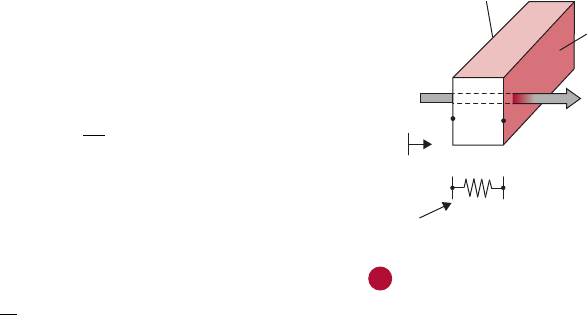
From everyday experience, we know that on a hot day, heat transfer

from the outside to the inside through the wall of a room (

Fig. 4.11)

depends on the surface area of the wall (a wall with larger surface area

will conduct more heat), the thermal properties of construction materi-

als (steel will conduct more heat than brick), wall thickness (more heat

transfer through a thin wall than thick), and temperature difference

(more heat transfer will occur when the outside temperature is much

hotter than the inside room temperature). In other words, the rate of

heat transfer through the wall may be expressed as

q ~

ðwall surface areaÞðtemperature differenceÞ

ðwall thicknessÞ

ð4:15Þ

Wall cross-section

Wall thickness

Length

Height

Heat transfe

Outside

Inside

Temperature

difference

Wall surface

area  Length 

Height

■ Figure 4.11 Conductive heat flow in a wall.

2834.3 Modes of Heat Transfer

A dT

ð4:16Þ

or, by inserting a constant of proportionality,

52kA

ð4:17Þ

where q

is the rate of heat flow in the direction of heat transfer by con-

duction (W); k is thermal conductivity (W/[m 8C] ); A is area (normal

to the direction of heat transfer) through which heat flows (m

); T is

temperature (8C); and x is length (m), avariable.

Equation (4.17) is also called Fourier’s law for heat conduction,

after Joseph Fourier, a French mathematical physicist. According to the

second law of thermodynamics, heat will always conduct from higher

temperature to lower temperature. As shown in Figure 4.12, the gradient

dT/dx is negative, because temperature decreases with increasing values

of x.Therefore, in Equation (4.17), a negative sign is used to obtain a

positive value for heat flow in the direction of decreasing temperature.

Example 4.3

One face of a stainless-steel plate 1 cm thick is maintained at 1108C,

and the other face is at 908C(

Fig. E4.3). Assuming steady-state conditions,

calculate the rate of heat transfer per unit area through the plate. The

thermal conductivity of stainless steel is 17 W/(m 8C).

Given

Thickness of plate 5 1cm5 0.01 m

Temperature of one face 5 1108C

Temperature of other face 5 908C

Thermal conductivity of stainless steel 5 17 W/(m 8C)

Approach

For steady-state heat transfer in rectangular coordinates we will use

Equation (4.17) to compute rate of heat transfer.

Solution

1. From Equation (4.17)

q 52

17 [W=(m 8C)] 3 1[m

] 3 (110 2 90) [8C]

(0 2 0:01) [m]

5 34, 000 W

T(x)

ΔT

Δx

Temperature (T )

Distance (x)



■ Figure 4.12 Sign convention for conductive

heat flow.

110°C

90°C

1 cm

■ Figure E4.3 Heat flow in a plate.

284 CHAPTER 4 Heat Transfer in Food Processing

2. Rate of heat transfer per unit area is calculated to be 34,000 W. A positive

sign is obtained for the heat transfer, indicating that heat always flows

“downhill” from 1108Cto908C.

4.3.2 Convective Heat Transfer

When a fluid (liquid or gas) comes into contact with a solid body

such as the surface of a wall, heat exchange will occur between the

solid and the fluid whenever there is a temperature difference between

the two. During heating and cooling of gases and liquids the fluid

streams exchange heat with solid surfaces by convection.

The magnitude of the fluid motion plays an important role in con-

vective heat transfer. For example, if air is flowing at a high velocity

past a hot baked potato, the latter will cool down much faster than if

the air velocity was much lower. The complex behavior of fluid flow

next to a solid surface, as seen in velocity profiles for laminar and

turbulent flow conditions in Chapter 2, make the determination of

convective heat transfer a complicated topic.

Depending on whether the flow of the fluid is artificially induced or

natural, there are two types of convective heat transfer: forced con-

vection and free (also called natural) convection. Forced convection

involves the use of some mechanical means, such as a pump or a

fan, to induce movement of the fluid. In contrast, free convection

occurs due to density differences caused by temperature gradients

within the system. Both of these mechanisms may result in either

laminar or turbulent flow of the fluid, although turbulence occurs

more often in forced convection heat transfer.

Consider heat transfer from a heated flat plate, PQRS, exposed to a

flowing fluid, as shown in

Figure 4.13. The surface temperature of

the plate is T

, and the temperature of the fluid far away from the

plate surface is T

. Because of the viscous properties of the fluid, a

velocity profile is set up within the flowing fluid, with the fluid

velocity decreasing to zero at the solid surface. Overall, we see that

the rate of heat transfer from the solid surface to the flowing fluid is

proportional to the surface area of solid, A, in contact with the fluid,

and the difference between the temperatures T

and T

.Or,

q ~ AðT

2 T

Þð4:18Þ

or,

q 5 hAðT

2 T

Þð4:19Þ

T∞

Fluid flow

■ Figure 4.13 Convective heat flow from the

surface of a flat plate.

2854.3 Modes of Heat Transfer

The area is A (m

), and h is the convective heat-transfer coefficient

(sometimes called surface heat-transfer coefficient), expressed as

W/(m

8C). This equation is also called Newton’s law of cooling.

Note that the convective heat transfer coefficient, h, is not a property

of the solid material. This coefficient, however, depends on a number

of properties of fluid (density, specific heat, viscosity, thermal conduc-

tivity), the velocity of fluid, geometry, and roughness of the surface of

the solid object in contact with the fluid.

Table 4.1 gives some approx-

imate values of h. A high value of h reflects a high rate of heat transfer.

Forced convection offers a higher value of h than free convection. For

example, you feel cooler sitting in a room with a fan blowing air than

in a room with stagnant air.

Example 4.4

The rate of heat transfer per unit area from a metal plate is 1000 W/m

The surface temperature of the plate is 1208C, and ambient temperature

is 208C(

Fig. E4.4). Estimate the convective heat transfer coefficient.

Given

Plate surface temperature 5 1208C

Ambient temperature 5 208C

Rate of heat transfer per unit area 5 1000 W/m

Approach

Since the rate of heat transfer per unit area is known, we will estimate the

convective heat transfer coefficient directly from Newton’s law of cooling,

Equation (4.19).

Table 4.1 Some Approximate Values of Convective Heat-Transfer

Coefficient

Fluid

Convective heat-transfer coefficient

(W/[m

K])

Air

Free convection 525

Forced convection 10200

Water

Free convection 20100

Forced convection 5010,000

Boiling water 3000100,000

Condensing water vapor 5000100,000

20°C

120°C

1000 W/m

■ Figure E4.4 Convective heat transfer from

a plate.

286 CHAPTER 4 Heat Transfer in Food Processing

Solution

1. From Equation (4.19),

h 5

1000[W=m

]

(120 2 20) [8C]

5 10 W=(m

8C)

2. The convective heat transfer coefficient is found to be 10 W/(m

8C).

4.3.3 Radiation Heat Transfer

Radiation heat transfer occurs between two surfaces by the emission

and later absorption of electromagnetic waves (or photons). In con-

trast to conduction and convection, radiation requires no physical

medium for its propagation—it can even occur in a perfect vacuum,

moving at the speed of light, as we experience everyday solar radia-

tion. Liquids are strong absorbers of radiation. Gases are transparent

to radiation, except that some gases absorb radiation of a particular

wavelength (for example, ozone absorbs ultraviolet radiation). Solids

are opaque to thermal radiation. Therefore, in problems involving

thermal radiation with solid materials, such as with solid foods, our

analysis is concerned primarily with the surface of the material. This

is in contrast to microwave and radio frequency radiation, where the

wave penetration into a solid object is significant.

All objects at a temperature above 0 Absolute emit thermal radiation.

Thermal radiation emitted from an object ’s surface is proportional to

the absolute temperature raised to the fourth power and the surface

characteristics. More specifically, the rate of heat emission (or radia-

tion) from an object of a surface area A is expressed by the following

equation:

q 5 σεAT

ð4:20Þ

where σ is the StefanBoltzmann

constant, equal to 5.669 3

W/(m

); T

is temperature, Absolute; A is the area (m

); and

Josef Stefan (18351893). An Austrian physicist, Stefan began his academic

career at the University of Vienna as a lecturer. In 1866, he was appointed direc-

tor of the Physical Institute. Using empirical approaches, he derived the law

describing radiant energy from blackbodies. Five years later, another Austrian,

Ludwig Boltzmann, provided the thermodynamic basis of what is now known

as the StefanBoltzmann law.

2874.3 Modes of Heat Transfer

ε is emissivity, which describes the extent to which a surface is similar to

a blackbody. For a blackbody, the value of emissivity is 1. Table A.3.3

gives values of emissivity for selected surfaces.

Example 4.5

Calculate the rate of heat energy emitted by 100 m

of a polished iron

surface (emissivity 5 0.06) as shown in

Figure E4.5. The temperature of the

surface is 378C.

Given

Emissivity ε 5 0.06

Area A 5 100 m

Temperature 5 378C 5 310 K

Approach

We will use the StefanBoltzmann law, Equation (4.20), to calculate the rate

of heat transfer due to radiation.

Solution

1. From Equation (4.20)

q 5 (5:669 3 10

W=[m

])(0:06)(100 m

)(310 K)

5 3141 W

2. The total energy emitted by the polished iron surface is 3141 W.

4.4 STEADY-STATE HEAT TRANSFER

In problems involving heat transfer, we often deal with steady state

and unsteady state (or transient) conditions. Steady-state conditions

imply that time has no influence on the temperature distribution

within an object, although temperature may be different at different

locations within the object. Under unsteady-state conditions, the

temperature changes with location and time. For example, consider

the wall of a refrigerated warehouse as shown in

Figure 4.14. The

inside wall temperature is maintained at 68C using refrigeration,

while the outside wall temperature changes throughout the day and

night. Assume that for a few hours of the day, the outside wall tem-

perature is constant at 208C, and during that time duration the rate

of heat transfer into the warehouse through the wall will be under

steady-state conditions. The temperature at any location inside the

wall cross-section (e.g., 148C at location A) will remain constant,

100 m

ε  0.06

37°C

■ Figure E4.5 Heat transfer from a plate.

6°C

8°C

10°C

12°C

14°C

16°C

18°C

20°C

Refrigerated

room

Outside

■ Figure 4.14 Steady state conductive heat

transfer in a wall.

288 CHAPTER 4 Heat Transfer in Food Processing

although this temperature is different from other locations along

the path of heat transfer within the wall, as shown in Figure 4.14.If,

however, the temperature of the outside wall surface changes (say,

increases above 208C), then the heat transfer through the wall will be

due to unsteady-state conditions, because now the temperature within

the wall will change with time and location. Although true steady-

state conditions are uncommon, their mathematical analysis is much

simpler. Therefore, if appropriate, we assume steady-state conditions

for the analysis of a given problem to obtain useful information for

designing equipment and processes. In certain food processes such as

in heating cans for food sterilization, we cannot use steady-state

conditions, because the duration of interest is when the temperature

is changing rapidly with time, and microbes are being killed. For ana-

lyzing those types of problems, an analysis involving unsteady-state

heat transfer is used, as discussed later in Section 4.5.

Another special case of heat transfer involves change in temperature

inside an object with time but not with location, such as might occur

during heating or cooling of a small aluminum sphere, which has a

high thermal conductivity. This is called a lumped system. We will

discuss this case in more detail in Section 4.5.2.

In the following section, we will examine several applications of

steady-state conduction heat transfer.

4.4.1 Conductive Heat Transfer

in a Rectangular Slab

Consider a slab of constant cross-sectional area, as shown in

Figure 4.15. The temperature, T

, on side X is known. We will develop

an equation to determine temperature, T

, on the opposite side Y and

at any location inside the slab under steady-state conditions.

This problem is solved by first writing Fourier’s law,

52kA

ð4:21Þ

The boundary conditions are

x 5 x

T 5 T

x 5 x

T 5 T

ð4:22Þ

Separating variables in

Equation (4.21), we get

dx 52kdT ð4:23Þ

Side Y

Side X

Thermal

resistance circuit

■ Figure 4.15 Heat transfer in a wall, also

shown with a thermal resistance circuit.

2894.4 Steady-S tate Heat Transfer

Setting up integration and substituting limits, we have

dx 52

kdT ð4:24Þ

Since q

and A are independent of x, and k is assumed to be indepen-

dent of T,

Equation (4.24) can be rearranged to give

dx 52k

dT ð4:25Þ

Finally, integrating this equation, we get

ðx

2 x

Þ52kðT

2 T

Þð4:26Þ

52kA

ðT

2 T

ðx

2 x

ð4:27Þ

Temperature on face Y is T

; thus, rearranging Equation (4.27),

5 T

ðx

2 x

Þð4:28Þ

To determine temperature, T, at any location, x, within the slab, we

may replace T

and x

with unknown T and distance variable x,

respectively, in

Equation (4.28) and obtain,

T 5 T

ðx 2 x

Þð4:29Þ

4.4.1.1 Thermal Resistance Concept

We noted in Chapter 3 that, according to Ohm’s Law, electrical cur-

rent, I, is directly proportional to the voltage difference, E

, and indi-

rectly proportional to the electrical resistance R

.Or,

I 5

ð4:30Þ

290 CHAPTER 4 Heat Transfer in Food Processing

If we rearrange the terms in Equation (4.27), we obtain

ðT

2 T

ðx

2 x



ð4:31Þ

or,

2 T

ð4:32Þ

Comparing

Equations (4.30) and (4.32) , we note an analogy

between rate of heat transfer, q

, and electrical current, I, temperature

difference, (T

2 T

) and electrical voltage, E

, and thermal resistance,

, and electrical resistance, R

. From Equations (4.31) and (4.32),

thermal resistance may be expressed as

ðx

2 x

ð4:33Þ

A thermal resistance circuit for a rectangular slab is also shown in

Figure 4.15. In solving problems involving conductive heat transfer in

a rectangular slab using this concept, we first obtain thermal resistance

using Equation (4.33) and then substitute it in Equation (4.32).The

rates of heat transfer across the two surfaces of a rectangular slab are

thus obtained. This procedure is illustrated in Example 4.6. The advan-

tage of using the thermal resistance concept will become clear when

we study conduction in multilayer walls. Moreover, the mathematical

computations will be much simpler compared with alter-native proce-

dures used in solving these problems.

Example 4.6

a. Redo Example 4.3 using the thermal resistance concept.

b. Determine the temperature at 0.5 cm from the 1108C temperature face.

Given

See Example 4.3

Location at which temperature is desired 5 0.5 cm 5 0.005 m

Approach

We will use Equation (4.33) to calculate thermal resistance, and then Equation

(4.32) to determine the rate of heat transfer. To determine temperature within the

slab, we will calculate the thermal resistance for the thickness of the slab bounded

2914.4 Steady-S tate Heat Transfer

by 1108C and the unknown temperature (Fig. E4.6). Since the steady-state heat

transfer remains the same throughout the slab, we will use the previously calcu-

lated value of q to determine the unknown temperature using Equation (4.32).

Solution

Part (a)

1. Using

Equation (4.33) , the thermal resistance R

0:01 [m]

17 [W=(m 8C)] 3 1[m

]

5 5:88 3 10

8C=W

2. Using

Equation (4.32) , we obtain rate of heat transfer as

q 5

110 [8C] 2 90 [8 C]

5:88 3 10

[8C=W]

q 5 34,013 W

Part (b)

3. Using

Equation (4.33) calculate resistance R

0:005 [m]

17 [W=(m 8C)] 3 1[m

]

5 2:94 3 10

8C=W

4. Rearranging terms in

Equation (4.32) to determine the unknown

temperature T

T 5 T

2 (q 3 R

)

T 5 110 [8C] 2 34,013 [W] 3 2:94 3 10

[8C=W]

T 5 1008C

5. The temperature at the midplane is 1008C. This temperature was

expected, since the thermal conductivity is constant, and the temperature

profile in the steel slab is linear.

4.4.2 Conductive Heat Transfer through a

Tubular Pipe

Consider a long, hollow cylinder of inner radius r

, outer radius r

and length L, as shown in

Figure 4.16.Lettheinsidewalltemperature

be T

and the outside wall temperature be T

. We want to calculate the

110°C

90°C

110°C

90°C

(a)

(b)

110°C

90°C

110°C

90°CT

0.5 cm 0.5 cm

■ Figure E4.6 Thermal resistance circuits for

heat transfer through a wall.

292 CHAPTER 4 Heat Transfer in Food Processing

rate of heat transfer along the radial direction in this pipe. Assume ther-

mal conductivity of the metal remains constant with temperature.

Fourier’s law in cylindrical coordinates may be written as

52kA

ð4:34Þ

where q

is the rate of heat transfer in the radial direction.

Substituting for circumferential area of the pipe,

52kð2πrLÞ

ð4:35Þ

The boundary conditions are

T 5 T

r 5 r

T 5 T

r 5 r

ð4:36Þ

Rearranging

Equation (4.35), and setting up the integrals,

2πL

52k

dT ð4:37Þ

Equation (4.37) gives

2πL

jln rj

52kjTj

ð4:38Þ

2πLkðT

2 T

lnðr

ð4:39Þ

■ Figure 4.16 Heat transfer in a radial

direction in a pipe, also shown with a thermal

resistance circuit.

2934.4 Steady-S tate Heat Transfer

Again, we can use the electrical resistance analogy to write an expres-

sion for thermal resistance in the case of a cylindrical-shaped object.

Rearranging the terms in

Equation (4.39), we obtain

ðT

2 T

lnðr

2πLk



ð4:40Þ

Comparing Equation (4.40) with Equation (4.32), we obtain the

thermal resistance in the radial direction for a cylinder as

lnðr

2πLk

ð4:41Þ

Figure 4.16 shows a thermal circuit to obtain R

. An illustration of

the use of this concept is given in Example 4.7.

Example 4.7

A 2-cm-thick steel pipe (thermal conductivity 5 43 W/[m 8C]) with 6 cm

inside diameter is being used to convey steam from a boiler to process

equipment for a distance of 40 m. The inside pipe surface temperature is

1158C, and the outside pipe surface temperature is 908C(

Fig. E4.7). Calculate

the total heat loss to the surroundings under steady-state conditions.

90°C

115°C

40 m

0.05 m

0.03 m

90°C

115°C

6 cm

10 cm

115°C90°C

End cross-section

Pipe thickness

■ Figure E4.7 Thermal resistance circuit for

heat transfer through a pipe.

294 CHAPTER 4 Heat Transfer in Food Processing

Given

Thickness of pipe 5 2cm5 0.02 m

Inside diameter 5 6cm5 0.06 m

Thermal conductivity k 5 43 W/(m 8C)

Length L 5 40 m

Inside temperature T

5 1158C

Outside temperature T

5 908C

Approach

We will determine the thermal resistance in the cross-section of the pipe and

then use it to calculate the rate of heat transfer, using

Equation (4.40) .

Solution

1. Using Equation (4.41)

ln(0:05=0:03)

2π 3 40[m] 3 43[W=(m 8C)]

5 4:727 3 10

8C=W

2. From

Equation (4.40)

q 5

115[8C] 2 90[8C]

4:727 3 10

[8C=W]

5 528,903 W

3. The total heat loss from the 40 m long pipe is 528,903 W.

4.4.3 Heat Conduction in Multilayered Systems

4.4.3.1 Composite Rectangular Wall (in Series)

We will now consider heat transfer through a composite wall made

of several materials of different thermal conductivities and thicknesses.

An example is a wall of a cold storage, constructed of different layers of

materials of different insulating properties. All materials are arranged in

series in the direction of heat transfer , as shown in

Figure 4.17.

From Fourier’s law,

q 52kA

This may be rewritten as

ΔT 52

qΔx

ð4:42Þ

2954.4 Steady-S tate Heat Transfer

Thus, for materials B, C, and D, we have

ΔT

qΔx

ΔT

qΔx

ΔT

qΔx

ð4:43Þ

From

Figure 4.17,

ΔT 5 T

2 T

5 ΔT

1 ΔT

ð4:44Þ

From

Equations (4.42), (4.43), and (4.44),

2 T

qΔx



ð4:45Þ

or, rearranging the terms,

2 T

Δx



ð4:46Þ

We can rewrite

Equation (4.46) for thermal resistance as

q 5

2 T

Δx



ð4:47Þ

or, using thermal resistance values for each layer, we can write

Equation (4.47) as,

q 5

2 T

1 R

ð4:48Þ

Δx

Area

■ Figure 4.17 Conductive heat transfer in a

composite rectangular wall, also shown with

a thermal resistance circuit.

296 CHAPTER 4 Heat Transfer in Food Processing

where

Δx

The thermal circuit for a multilayer rectangular system is shown in

Figure 4.17. Example 4.8 illustrates the calculation of heat transfer

through a multilayer wall.

Example 4.8

A cold storage wall (3 m 3 6 m) is constructed of 15-cm-thick concrete

(thermal conductivity 5 1.37 W/[m 8C]). Insulation must be provided to

maintain a heat transfer rate through the wall at or below 500 W (

Fig. E4.8).

If the thermal conductivity of the insulation is 0.04 W/(m 8C), compute the

required thickness of the insulation. The outside surface temperature of

the wall is 388C, and the inside wall temperature is 58C.

Given

Wall dimensions 5 3m3 6m

Thickness of concrete wall 5 15 cm 5 0.15 m

concrete

5 1.37 W/(m 8C)

Maximum heat gain permitted, q 5 500 W

insulation

5 0.04 W/(m 8C)

Outer wall temperature 5 388C

Inside wall (concrete/insulation) temperature 5 58C

Approach

In this problem we know the two surface temperatures and the rate of heat trans-

fer through the composite wall, therefore, using this information we will first

calculate the thermal resistance in the concrete layer. Then we will calculate the

thermal resistance in the insulation layer, which will yield the thickness value.

Solution

1. Using Equation (4.48)

q 5

(38 2 5)[8 C]

1 R

2. Thermal resistance in the concrete layer, R

0:15 [m]

1:37 [W=(m 8C)] 3 18 [m

]

5 0:00618C=W

38°C

5°C

38°C

5°C

500 W

15 cm

■ Figure E4.8 Heat transfer through a

two-layered wall.

2974.4 Steady-S tate Heat Transfer

3. From step 1,

(38 2 5)[8C]

1 0:0061[8C=W]

5 500

or,

(38 2 5)[8C]

500[W]

5 0:0061[8C=W]

5 0:068C=W

4. From

Equation (4.48)

Δx

5 R

Thickness of insulation 5 0:06 [8C=W] 3 0:04[W=(m 8C)] 3 18 [m

]

5 0:043 m 5 4:3cm

5. An insulation with a thickness of 4.3 cm will ensure that heat loss from

the wall will remain below 500 W. This thickness of insulation allows a

91% reduction in heat loss.

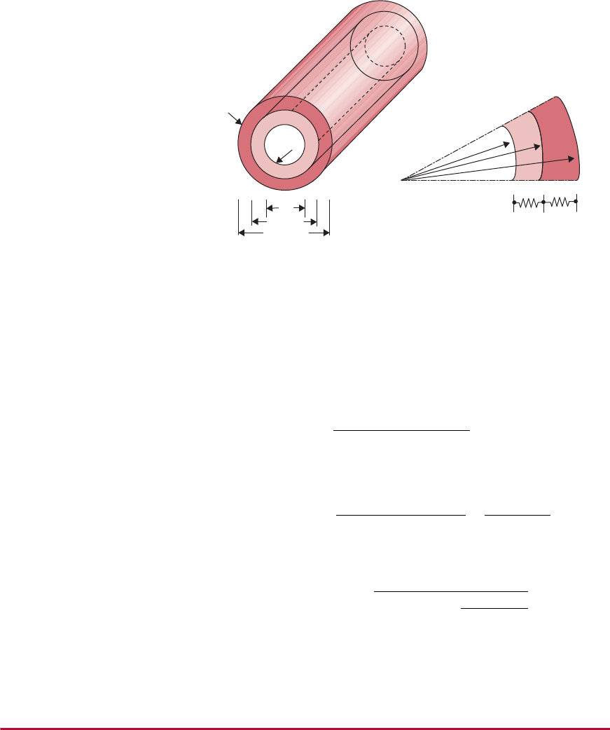
4.4.3.2 Composite Cylindrical Tube (in Series)

Figure 4.18 shows a composite cylindrical tube made of two layers of

materials, A and B. An example is a steel pipe covered with a layer

of insulating material. The rate of heat transfer in this composite

tube can be calculated as follows.

In Section 4.4.2 we found that rate of heat transfer through a single-

wall cylinder is

2 T

)

ln(r

)

2πLk



The rate of heat transfer through a composite cylinder using thermal

resistances of the two layers is

2 T

)

1 R

ð4:49Þ

or, substituting the individual thermal resistance values,

2 T

)

ln(r

)

2πLk

ln(r

)

2πLk

ð4:50Þ

298 CHAPTER 4 Heat Transfer in Food Processing

The preceding equatio n is useful in calculating the rate of heat

transfer through a multilayered cylinder. Note that if there were

three laye rs present between the two su rfaces with temperatures T

and T

, then we just add another thermal resistance term in the

denominator.

Suppose we need to know the temperature at the interface between

two layers, T

, as shown in Figure 4.18. First, we calculate the steady-

state rate of heat transfer using Equation (4.50), noting that under

steady-state conditions, q

has the same value through each layer of

the composite wall. Then, we can use the following equation, which

represents the thermal resistance between the known temperature, T

and the unknown temperature, T

5 T

2 q

ln(r

)

2πLk



ð4:51Þ

This procedure to solve problems for unknown interfacial tempera-

tures is illustrated in Example 4.9.

■ Figure 4.18 Conductive heat transfer in concentric cylindrical pipes, also shown with a thermal resistance circuit.

2994.4 Steady-S tate Heat Transfer

Example 4.9

A stainless-steel pipe (thermal conductivity 5 17 W/[m 8C]) is being used

to convey heated oil (

Fig. E4.9). The inside surface temperature is 1308C.

The pipe is 2 cm thick with an inside diameter of 8 cm. The pipe is insu-

lated with 0.04-m-thick insulation (thermal conductivity 5 0.035 W/[m 8C]).

The outer insulation temperature is 258C. Calculate the temperature of the

interface between steel and insulation , assume steady-state conditions.

Given

Thickness of pipe 5 2cm5 0.02 m

Inside diameter 5 8cm5 0.08 m

steel

5 17 W/(m 8C)

Thickness of insulation 5 0.04 m

insulation

5 0.035 W/(m 8C)

Inside pipe surface temperature 5 1308C

Outside insulation surface temperature 5 258C

Pipe length 5 1 m (assumed)

Approach

We will first calculate the two thermal resistances, inthepipeandtheinsulation.

Then we will obtain the rate of heat transfer through the composite layer. Finally ,

we will use the thermal resistance of the pipe alone to determine the temperature

at the interface between the pipe and insulation.

Solution

1. Thermal resistance in the pipe layer is, from Equation (4.41),

ln(0:06=0:04)

2π 3 1[m] 3 17 [W=(m 8C)]

5 0:0038 8C=W

10 cm

6 cm

4 cm

130°C

25°C

8 cm

12 cm

20 cm

25°C

130°C

■ Figure E4.9 Heat transfer through a

multilayered pipe.

300 CHAPTER 4 Heat Transfer in Food Processing

2. Similarly, the thermal resistance in the insulation layer is,

ln(0:1=0:06)

2π 3 1[m]3 0:035 [W=(m 8C)]

5 2:3229 8C=W

3. Using

Equation (4.49) , the rate of heat transfer is

q 5

(130 2 25)[8C]

0:0038 [8C=W] 1 2:3229 [8C=W]

5 45:13 W

4. Using

Equation (4.40)

45:13 [W] 5

(130 2 T)[8C]

0:0038 [8C=W]

T 5 130 [8C] 2 0:171 [8C]

T 5 129:838C

5. The interfacial temperature is 129.88C. This temperature is very close to

the inside pipe temperature of 1308C, due to the high thermal con-

ductivity of the steel pipe. The interfacial temperature between a hot

surface and insulation must be known to ensure that the insulation

will be able to withstand that temperature.

Example 4.10

A stainless-steel pipe (thermal conductivity 5 15 W/[mK]) is being used to

transport heated oil at 1258C(

Fig. E4.10).Theinsidetemperatureofthepipeis

1208C. The pipe has an inside diameter of 5 cm and is 1 cm thick. Insulation

is necessary to keep the heat loss from the oil below 25 W/m length of the

pipe. Due to space limitations, only 5-cm-thick insulation can be provided. The

outside surface temperature of the insulation must be above 208C(thedew

point temperature of surrounding air) to avoid condensation of water on the

surface of insulation. Calculate the thermal conductivity of insulation that will

result in minimum heat loss while avoiding water condensation on its surface.

Given

Thermal conductivity of steel 5 15 W/(m K)

Inside pipe surface temperature 5 1208C

Inside diameter 5 0.05 m

Pipe thickness 5 0.01 m

Heat loss permitted in 1 m length of pipe 5 25 W

Insulation thickness 5 0.05 m

Outside surface temperature . 208C 5 218C (assumed)

3014.4 Steady-S tate Heat Transfer

Approach

We will first calculate the thermal resistance in the steel layer, and set up an

equation for the thermal resistance in the insulation layer. Then we will sub-

stitute the thermal resistance values into

Equation (4.50). The only unknown,

thermal conductivity, k, will be then calculated.

Solution

1. Thermal resistance in the steel layer is

ln(3:5=2:5)

2π 3 1[m]3 15 [W=(m 8C)

5 0:0036 8C=W

2. Thermal resistance in the insulation layer is

ln(8:5=3:5)

2π 3 1[m]3 k[W=(m 8C)

0:1412[1=m]

k[W=(m 8C)]

3. Substituting the two thermal resistance values in

Equation (4.50)

25[W] 5

(120 2 21)[8C]

0:0036[8C=W] 1

0:1412 [1=m]

k[W=(m 8C)]

or,

k 5 0:0357 W=(m 8 C)

4. An insulation with a thermal conductivity of 0.0357 W/(m 8C) will ensure

that no condensation will occur on its outer surface.

8.5 cm

3.5 cm

2.5 cm

120°C

20°C

5 cm

7 cm

17 cm

20°C

120°C

■ Figure E4.10 Heat transfer through a

multilayered pipe.

302 CHAPTER 4 Heat Transfer in Food Processing

4.4.4 Estimation of Convective Heat-Transfer

Coefficient

In Section 4.3.1 on the conduction mode of heat transfer, we observed

that any material undergoing conduction heating or cooling remains

stationary. Conduction is the main mode of heat transfer within solids.

Now we will consider heat transfer between a solid and a surrounding

fluid, a mode of heat transfer called convection. In this case, the material

experiencing heating or cooling (a fluid) also moves. The movement of

fluid may be due to the natural buoyancy effects or caused by artificial

means, such as a pump in the case of a liquid or a blower for air.

Determination of the rate of heat transfer due to convection is compli-

cated because of the presence of fluid motion. In Chapter 2, we noted

that a velocity profile develops when a fluid flows over a solid surface

because of the viscous properties of the fluid material. The fluid next

to the wall does not move but “sticks” to it, with an increasing velocity

away from the wall. A boundary layer develops within the flowing

fluid, with a pronounced influence of viscous properties of the fluid.

This layer moves all the way to the center of a pipe, as was shown

in Figure 2.14. The parabolic velocity profile under laminar flow

conditions indicates that the drag caused by the sticky layer in contact

with the solid surface influences velocity at the pipe center.

Similar to the velocity profile, a temperature profile develops in a

fluid as it flows through a pipe, as sho wn in

Figure 4.19. Sup pose

the temperature of the p ipe surface is kept constant at T

, and the

fluid enters with a uniform temperature, T

. A temperature profile

develops because the fluid in contact with the pipe surface quickly

reaches the wall temperature, thus setting up a temperature gradient

as shown in the figure. A thermal boundary layer develops. At the

end of the thermal entrance region, the boundary layer extends all

the way to the pipe centerline.

Therefore, when heating or cooling a fluid as it flows through a

pipe, two boundar y layers d eve lop—a hydrodynami c boundary

Thermal entry region

Thermally

developed region

■ Figure 4.19 Thermal entry region in fluid

flowing in a pipe.

3034.4 Steady-S tate Heat Transfer

layer and a thermal boundary layer. These boundary layers have

a major influence on the rate of heat transfer between the pipe

surface and the fluid. The mathematics involved in an analytical

treatment of this subject is complicated and beyond the scope

of this book. However, there is an equal ly useful procedure called

the em pirical approach, which is widely used to determine the rate

of convective heat transfer. A drawback of the empiric al approach

is that it requires a large number of experiments to obtain the

required data. We overcome this problem and keep the data analy-

sis manageable by using dimensionless numbers. To formulate this

approach, first we will identify and review the required di mension-

less numbers: Reynolds number, N

, Nusselt number, N

, and

Prandtl number, N

The Reynolds number was described in Section 2.3.2. It provides an

indication of the inertial and viscous forces present in a fluid. The

Reynolds number is calculated using Equation (2.20).

The second required dimensionless number for our data analysis is

Nusselt number—the dimensionless form of convective heat transfer

coefficient, h. Consider a fluid layer of thickness l, as shown in

Figure 4.20. The temperature difference between the top and bottom

of the layer is ΔT. If the fluid is stationary, then the rate of heat trans-

fer will be due to conduction, and the rate of heat transfer will be

conduction

52kA

ΔT

ð4:52Þ

However, if the fluid layer is moving, then the heat transfer will be

due to convection, and the rate of heat transfer using Newton ’s law

of cooling will be

convection

5 hAΔT ð4:53Þ

Dividing

Equation (4.53) by (4.52), we get

convection

conduction

hAΔT

kAΔT=l

 N

ð4:54Þ

Replacing thickness l with a more general term for dimension, the

characteristic dimension d

, we get



ð4:55Þ

ΔT  T

 T

■ Figure 4.20 Heat transfer through a

fluid layer.

304 CHAPTER 4 Heat Transfer in Food Processing

Nusselt number may be viewed as an enhancement in the rate of

heat transfer caused by convection over the conduction mode.

Therefore, if N

5 1, then there is no improvement in the rate of

heat transfer due to convection. However, if N

5 5, the rate of con-

vective heat transfer due to fluid motion is five times the rate of heat

transfer if the fluid in contact with the solid surface is stagnant. The

fact that by blowing air over a hot surface we can cool it faster is

due to increased Nusselt number and consequently to an increased

rate of heat transfer.

The third required dimensionless number for the empirical approach

to determine convective heat transfer is Prandtl number, N

, which

describes the thickness of the hydrodynamic boundary layer com-

pared with the thermal boundary layer. It is the ratio between the

molecular diffusivity of momentum to the molecular diffusivity of

heat. Or,

molecular diffusivity of momentum

molecular diffusivity of heat

ð4:56Þ

or,

kinematic viscosity

thermal diffusivity

ð4:57Þ

Substituting

Equations (2.11) and (4.12) in Equation (4.57),

μc

ð4:58Þ

If N

5 1, then the thickness of the hydrodynamic and thermal

boundary layers will be exactly the same. On the other hand, if

{1, the molecular diffusivity of heat will be much larger than that

of momentum. Therefore, the heat will dissipate much faster, as in the

case of a liquid metal flowing in a pipe. For gases, N

is about 0.7,

and for water it is around 10.

With a basic understanding of these three dimensionless numbers,

we will now plan the following experiment to determine convective

rate of heat transfer. Assume that a fluid is flowing in a heated pipe.

We are interested in determining convective rate of heat transfer from

the inside surface of the heated pipe into the fluid flowing inside the

pipe, as shown in

Figure 4.21. We carry out this experiment by pump-

ing a fluid such as water, entering at a velocity of u

at a temperature

of T

and flowing parallel to the inside surface of the pipe. The pipe

3054.4 Steady-S tate Heat Transfer

is heated using an electrical heater so that the inside pipe surface is

maintained at temperature T

, which is higher than the inlet fluid

temperature, T

. We measure the electric current, I, and electrical resis-

tance, R

, and calculate the product of the two to determine the rate

of heat transfer, q. The pipe is well insulated so that all the electrically

generated heat transfers into the fluid. Thus, we can experimentally

determine values of q, A, T

, u

, and T

.UsingEquation (4.53), we can

calculate the convective heat transfer coefficient, h.

If we repeat this experiment with a different diameter pipe or differ-

ent temperature of pipe surface, a new value of h will be obtained.

It should become clear that we can perform a series of experiments

to obtain h values that are a function of the operating variables, q, A,

, T

, and T

. The disadvantage of this experiment is that a large

amount of experimental data are generated, and organizing these

data for meaningful applications is a daunting task. However, the

data analysis can be greatly simplified if we combine various proper-

ties and operating variables into the three dimensionless numbers,

, N

, and N

, which will accommodate all the properties and

variables that are important to our experiment.

Thus, for each experimental set, we calculate the respective dimension-

less numbers and, using log-log scale, plot the Nusselt number as a

function of the Reynolds number for different values of the Prandtl

number.

Figure 4.22 shows a typical plot. It has been experimentally

determined that for a given fluid with a fixed Prandtl number, straight

line plots are obtained on the log-log scale, as shown in Figure 4.22.

Fluid inlet

temperature  T

Velocity  u

Current I

Surface temperature T

■ Figure 4.21 Heating of fluid with electrically

heated pipe surface.

Log N

Pr1

Pr2

Pr3

 CN

■ Figure 4.22 A plot of Nusselt and Reynolds

numbers on a log-log scale.

306 CHAPTER 4 Heat Transfer in Food Processing

This type of graphical relationship may be conveniently expressed with

an equation as

5 CN

ð4:59Þ

where C, m, and n are coefficients.

By substituting the experimentally obtained coefficients in

Equation (4. 59), we ob tain empirical correlations specific for a given

condition. Several researchers have determined these empirical cor-

relations for a variety of ope rating conditions, such as fluid flow

inside a pipe, over a pipe, or over a sphere. Different corre lations

are obtained, depending on whether the flow is laminar or

turbulent.

A suggested methodology to solve problems requiring the calculation

of convective heat transfer coefficients using empirical correlations is

as follows:

1. Identify flow geometry. The first step in a calculation involving

convection heat transfer is to clearly identify the geometrical

shape of the solid surface in contact with the fluid and its

dimensions. For example, is it a pipe, sphere, rectangular duct,

or a rectangular plate? Is the fluid flowing inside a pipe or over

the outside surface?

2. Identify the fluid and determine its properties. The second step is

to identify the type of fluid. Is it water, air, or a liquid food?

Determine the average fluid temperature far away from the solid

surface, T

. In some cases the average inlet and outlet tempera-

tures may be different, for example, in a heat exchanger; in that

case calculate the average fluid temperature as follows:

1 T

ð4:60Þ

where T

is the average inlet fluid temperature and T

is the

average exit fluid temperature. Use the average fluid tempera-

ture, T

, to obtain physical and thermal properties of the fluid,

such as viscosity, density, and thermal conductivity, from appro-

priate tables (such as Table A.4.1 for water, Table A.4.4 for air),

paying careful attention to the units of each property.

3. Calculate the Reynolds number. Using the velocity of the fluid ,

fluid properties and the characteristic dimension of the object

3074.4 Steady-S tate Heat Transfer

in contact with the fluid, calculate the Reynolds number.

The Reynolds number is necessary to determine whether the

flow is laminar, transitional, or turbulent. This information is

required to select an appropriate empirical correlation.

4. Select an appropriate empirical correlation. Using the information

from steps (1) and (3), select an empirical correlation of the

form given in

Equation (4.59) for the conditions and geome-

try of the object that resembles the one being investigated

(as presented later in this section). For example, if the given

problem involves turbulent water flow in a pipe, select the

correlation given in Equation (4.67). Using the selected corre-

lation, calculate Nusselt number and finally the convective

heat transfer coefficient.

The convective heat-transfer coefficient h is predicted from empirical

correlations. The coefficient is influenced by such parameters as type

and velocity of the fluid, physical properties of the fluid, temperature

difference, and geometrical shape of the physical system under

consideration.

The empirical correlations useful in predicting h are presented in the

following sections for both forced and free convection. We will dis-

cuss selected physical systems that are most commonly encountered

in convective heat transfer in food processing. For other situations

refer to handbooks such as

Rotstein et al. (1997) or Heldman and

Lund (1992). All correlations apply to Newtonian fluids only. For

expressions for non-Newtonian fluids, the textbook by Heldman and

Singh (1981) is recommended.

4.4.4.1 Forced Convection

In forced convection, a fluid is forced to move over a solid surface

by external mechanical means, such as an electric fan, pump, or a

stirrer (Fig. 4.23). The general correlation between the dimensionless

numbers is

5 ΦðN

Þð4:61Þ

where N

is Nusselt number 5 hd

/k; h is convective heat-transfer coef-

ficient (W/[m

8C]); d

is the characteristic dimension (m); k is thermal

conductivity of fluid (W/[m 8C]); N

is Reynolds number 5 ρud

=μ;

ρ is density of fluid (kg/m

); u is velocity of fluid (m/s); μ is viscosity

(Pa s); N

is Prandtl number 5 μc

/k; c

is specific heat (kJ/[kg 8C]);

and Φ stands for “function of”.

Air flow

directed on

the external

surface of a

pipe

Air flow

directed on

the inside

surface of a

pipe

Fan

■ Figure 4.23 Forced convective heat

transfer from a pipe with flow inside and outside

the pipe.

308 CHAPTER 4 Heat Transfer in Food Processing

Laminar flow in pipes

1. Fully developed conditions with constant surface temperature

of the pipe:

5 3:66 ð4:62Þ

where thermal conductivity of the fluid is obtained at average

fluid temperature, T

, andd

is the inside diameter of the pipe.

2. Fully developed conditions with uniform surface heat flux:

5 4:36 ð4:63Þ

where thermal conductivity of the fluid is obtained at average

fluid temperature, T

, andd

is the inside diameter of the pipe.

3. For both entry region and fully developed flow conditions:

5 1:86 N

3 N



0:33



0:14

ð4:64Þ

where L is the length of pipe (m); characteristic dimension, d

is the inside diameter of the pipe; all physical properties are

evaluated at the average fluid temperature, T

, except μ

which is evaluated at the surface temperature of the wall.

Transition flow in pipes

For Reynolds numbers between 2100 and 10,000,

ðf =8ÞðN

2 1000ÞN

1 1 12:7ðf =8Þ

1=2

ðN

2=3

2 1Þ

ð4:65Þ

where all fluid properties are evaluated at the average fluid tempera-

ture, T

, d

is the inside diameter of the pipe, and the friction factor, f,

is obtained for smooth pipes using the following expression:

f 5

ð0:790 ln N

21:64Þ

ð4:66Þ

Turbulent flow in pipes

The following equation may be used for Reynolds numbers greater

than 10,000:

5 0:023N

0:8

3 N

0:33



0:14

ð4:67Þ

3094.4 Steady-S tate Heat Transfer

Fluid properties are evaluated at the average film temperature, T

except μ

, which is evaluated at the wall temperature; d

is the inside

diameter of the pipe.

Equation (4.67) is valid both for constant

surface temperature and uniform heat flux conditions.

Convection in noncircular ducts

For noncircular ducts, an equivalent diameter, D

, is used for the

characteristic dimension:

4 3 free area

wetted perimeter

ð4:68Þ

Figure 4.24 shows a rectangular duct with sides of length W and H.

The equivalent diameter in this case will be equal to 2 WH/(W 1 H).

Flow past immersed objects

In several applications, the fluid may flow past immersed objects. For

these cases, the heat transfer depends on the geometrical shape of the

object, relative position of the object, proximity of other objects, flow

rate, and fluid properties.

For a flow past a single sphere, when the single sphere may be heated

or cooled, the following equation will apply:

5 2 1 0:60N

0:5

3 N

1=3

for

1 , N

, 70,000

0:6 , N

, 400



ð4:69Þ

where the characteristic dimension, d

, is the outside diameter of the

sphere. The fluid properties are evaluated at the film temperature T

where

1 T

For heat transfer in flow past other immersed objects, such as cylinders

and plates, correlations are available in Perry and Chilton (1973).

Example 4.11

Water flowing at a rate of 0.02 kg/s is heated from 20 to 608C in a horizontal

pipe (inside diameter 5 2.5 cm). The inside pipe surface temperature is

908C(

Fig. E4.11). Estimate the convective heat-transfer coefficient if the pipe

is 1 m long.

■ Figure 4.24 Cross-section of a

rectangular duct.

310 CHAPTER 4 Heat Transfer in Food Processing

Given

Water flow rate 5 0.02 kg/s

Inlet temperature 5 208C

Exit temperature 5 608C

Inside diameter 5 2.5 cm 5 0.025 m

Inside pipe surface temperature 5 908C

Length of pipe 5 1m

Approach

Since water is flowing due to some external means, the problem indicates

forced convective heat transfer. We will first determine if the flow is laminar

by calculating the Reynolds number. If the Reynolds number is less than 2100,

we will use

Equation (4.64) to calculate the Nusselt number. From the Nusselt

number we will calculate the h value.

Solution

1. Physical properties of water are needed to calculate the Reynolds number.

All physical properties except u

must be evaluated at average bulk fluid

temperature, (20 1 60)/2 5 408C. From Table A.4.1 at 408C,

Density ρ 5 992.2 kg/m

Specific heat c

5 4.175 kJ/(kg 8C)

Thermal conductivity k 5 0.633 W/(m 8C)

Viscosity (absolute) μ 5 658.026 3 10

Pa s

Prandtl number N

5 4.3

Thus,

ρuD

πμD

(4)(0:02 kg=s)

(π)(658:026 3 10

P a s)(0:025 m)

5 1547:9

Note that 1 Pa 5 1kg/(ms

). Since the Reynolds number is less than 2100,

the flow is laminar.

2. We select

Equation (4.64), and using μ

5 308.909 3 10

Pa s at 908C,

5 1:86(1547:9 3 4:3 3 0:025)

0:33



658:016 3 10

308:909 3 10



0:14

5 11:2

2.5 cm

1 m

90°C

■ Figure E4.11 Convective heat transfer inside

a pipe.

3114.4 Steady-S tate Heat Transfer

3. The convective heat-transfer coefficient can be obtained from the Nusselt

number.

h 5

(11:2)(0:633 W=[m 8C])

(0:025 m)

5 284 W=(m

8C)

4. The convective heat-transfer coefficient is estimated to be 284 W/(m

8C).

Example 4.12

If the rate of water flow in Example 4.11 is raised to 0.2 kg/s from 0.02 kg/s

while all other conditions are kept the same, calculate the new convective

heat-transfer coefficient.

Given

See Example 4.11

New mass flow rate of water 5 0.2 kg/s

Approach

We will calculate the Reynolds number to find whether the flow is turbulent. If

the flow is turbulent, we will use

Equation (4.67) to compute the Nusselt number.

The surface heat-transfer coefficient will be computed from the Nusselt number.

Solution

1. First, we compute the Reynolds number using some of the properties

obtained in Example 4.11.

(4)(0:2kg=s)

(π)(658:026 3 10

Pa s)(0:025 m)

5 15, 479

Thus, flow is turbulent.

2. For turbulent flow, we select

Equation (4.67) .

5 ð0:023Þð15479Þ

0:8

ð4:3Þ

0:33

658:026 3 10

308:909 3 10

0:14

5 93

3. The convective heat transfer can be computed as

h 5

(93)(0:633 W=[m 8 C])

(0:025 m)

5 2355 W=(m

8C)

312 CHAPTER 4 Heat Transfer in Food Processing

4. The convective heat-transfer coefficient for turbulent flow is estimated

to be 2355 W/(m

8C). This value is more than eight times higher than

the value of h for laminar flow calculated in Example 4.11.

Example 4.13

What is the expected percent increase in convective heat-transfer coeffi-

cient if the velocity of a fluid is doubled while all other parameters are

kept the same for turbulent flow in a pipe?

Approach

We will use Equation (4.67) to solve this problem.

Solution

1. For turbulent flow in a pipe

5 0:023N

0:8

3 N

0:33



0:14

We can rewrite this equation as

5 f(u

)

0:8

5 f(u

)

0:8





0:8

2. Since u

5 2u

5 (2)

0:8

5 1:74

5 1:74N

3. This expression implies that h

5 1.74 h

. Thus,

%Increase 5

1:74h

2 h

3 100 5 74%

4. As expected, velocity has a considerable effect on the convective

heat-transfer coefficient.

3134.4 Steady-S tate Heat Transfer

Example 4.14

Calculate convective heat-transfer coefficient when air at 908C is passed

through a deep bed of green peas. Assume surface temperature of a pea

to be 308C. The diameter of each pea is 0.5 cm. The velocity of air through

the bed is 0.3 m/s.

Given

Diameter of pea 5 0.005 m

Temperature of air 5 908C

Temperature of a pea 5 308C

Velocity of air 5 0.3 m/s

Approach

Since the air flows around a spherically immersed object (green pea), we will

estimate N

from Equation (4.69). The Nusselt number will give us the value

for h.

Solution

1. The properties of air are evaluated at T

, where

1 T

30 1 90

5 608C

From Table A.4.4,

ρ 5 1:025 kg=m

5 1:017 kJ=(kg 8C)

k 5 0:0279 W=(m 8C)

μ 5 19:907 3 10

Pa s

5 0:71

2. The Reynolds number is computed as

(1:025 kg=m

)(0:3m=s)(0:005 m)

(19:907 3 10

Pa s)

5 77:2

3. From

Equation (4.69) ,

5 2 1 0:6(77:2)

0:5

(0:71)

0:33

5 6:71

314 CHAPTER 4 Heat Transfer in Food Processing

4. Thus

h 5

6:71(0:0279W=[m 8C])

(0:005 m)

5 37 W=(m

8C)

5. The convective heat-transfer coefficient is 37 W/(m

8C).

4.4.4.2 Free Convection

Free convection occurs because of density differences in fluids as they

come into contact with a heated surface (

Fig. 4.25). The low density

of fluid at a higher temperature causes buoyancy forces, and as a

result, heated fluid moves upward and colder fluid takes its place.

Empirical expressions useful in predicting convective heat-transfer

coefficients are of the following form:

5 aðN

ð4:70Þ

where a and m are constants; N

, is the Rayleigh number. Rayleigh

number is a product of two dimensionless numbers, Grashof number

and Prandtl number.

5 N

3 N

ð4:71Þ

The Grashof number, N

, is defined as follows:

gβΔT

ð4:72Þ

where d

is characteristic dimension (m); ρ is density (kg/m

); g is accel-

eration due to gravity (9.80665 m/s

); β is coefficient of volumetric

expansion (K

); ΔT is temperature difference between wall and the

surrounding bulk (8C); and μ is viscosity (Pa s).

A Grashof number is a ratio between the buoyancy forces and

viscous forces. Similar to the Reynolds number, the Grashof number

is useful for determining whether a flow over an object is laminar or

turbulent. For example, a Grashof number greater than 10

for fluid

flow over vertical plates signifies a turbulent flow.

In the case of heat transfer due to free convection, physical properties

are evaluated at the film temperature, T

5 (T

1 T

)/2.

Table 4.2 gives various constants that may be used in Equation (4.70)

for natural convection from vertical plates and cylinders, and from

horizontal cylinders and plates.

Air flow

around a pipe

due to a natural

convection

Pipe with a

heated outside

surface

■ Figure 4.25 Heat transfer from the outside

of a heated pipe due to natural convection.

3154.4 Steady-S tate Heat Transfer

Table 4.2 Coefficients for Equation (4.70) for Free Convection

Geometry

Characteristic

Length Range of N

amEquation

Vertical plate L 10

10

0.59 0.25 N

5 a(N

)

10

0.1 0.333

Inclined plate L Use same equations as vertical plate,

replace g by g cos θ for N

, 10

Horizontal plate A/p 10

10

0.54 0.25 N

5 a(N

)

Surface area 5 A 10

10

0.15 0.33

Perimeter 5 p

(a) Upper surface of

a hot plate (or lower

surface of a cold plate)

Hot surface

Horizontal plate A/p 10

10

0.27 0.25 N

5 a(N

)

Surface area 5 A

Perimeter 5 p

(b) Lower surface of

a hot plate (or upper

surface of a cold plate)

Hot surface

(Continued)

316 CHAPTER 4 Heat Transfer in Food Processing

Example 4.15

Estima te the convective heat-trans fer coefficient for convective heat

loss from a horizontal 10 cm diameter steam pipe. The surface tempera-

ture of the uninsulated pipe is 1308C, and the air temperature is 308 C

(

Fig. E4.12).

Given

Diameter of pipe 5 10 cm 5 0.1 m

Pipe surface temperature T

5 1308C

Ambient temperature T

5 308C

Table 4.2 (Continued)

Geometry

Characteristic

Length Range of N

amEquation

Vertical cylinder

L A vertical cylinder can be treated as a

vertical plate when

D $

35L

0:25

Horizontal cylinder

D 10

10

212

5 0:61

0:387N

1=6

0:559



9=16

8=27

;

Sphere

πD

# 10

$ 0.7)

5 2 1

0:589N

1=4

0:469



9=16

4=9

3174.4 Steady-S tate Heat Transfer

Approach

Since no mechanical means of moving air are indicated, heat loss from the

horizontal pipe is by free convection. After finding the property values of air

at film temperature, we will calculate the Grashof number. The product of the

Grashof number and Prandtl number will allow determination of a and m

parameters from

Table 4.2; these parameters will be used in Equation (4.72).

We will then compute the surface heat-transfer coefficient from the Nusselt

number.

Solution

1. Since no mechanical means of moving the air are indicated, heat loss

is by free convection.

2. The film temperature is obtained as

1 T

130 1 30

5 808C

3. The properties of air at 808C are obtained from Table A.4.4.

ρ 5 0:968 kg=m

β 5 2:83 3 10

5 1:019 kJ=(kg 8C)

k 5 0:0293 W=(m 8C)

μ 5 20:79 3 10

Ns=m

5 0:71

g 5 9:81 m=s

4. We calculate Rayleigh number, N

, the product of N

and N

. The

characteristic dimension is the outside diameter of the pipe.

gβΔT

(0:1m)

(0:968 kg=m

)

(9:81 m=s

)(2:833 10

)(1308C 2 308C)

(20:793 1026Ns=m

)

5 6:0193 10

(Note that 1 N 5 kg m/s

.) Thus,

3 N

5 (6:019 3 10

)(0:71) 5 4:27 3 10

10 cm

130°C

30°C

■ Figure E4.12 Convective heat transfer from

a horizontal pipe.

318 CHAPTER 4 Heat Transfer in Food Processing

5. From Table 4.2, for horizontal cylinder

5 0:61

0:387(4:27 3 10

)

1=6

0:559

0:71



9=16

8=27

6. N

5 22

7. Thus

h 5

(22)(0:0293 W=[m 8C])

(0:1m)

5 6:5W=(m

8C)

4.4.4.3 Thermal Resistance in Convective Heat Transfer

A thermal resistance term for convective heat transfer may be defined

in a similar manner as in conductive heat transfer (

Section 4.4).

From Equation (4.19), we know that

q 5 hAðT

2 T

Þð4:73Þ

or, rearranging terms in

Equation (4.73),

q 5

2 T



ð4:74Þ

where the thermal resistance due to convection (R

)

convection

ðR

convection

ð4:75Þ

In problems involving conduction and convection heat transfer in

series, along the path of heat transfer, the thermal resistance due to

convection is added to the thermal resistance due to conduction

to obtain the total thermal resistance. We will discuss this further

in the context of overall heat transfer involving both conduction and

convection heat transfer.

3194.4 Steady-S tate Heat Transfer

4.4.5 Estimation of Overall Heat-Transfer Coefficient

In many heating/cooling applications, conductive and convective heat

transfer may occur simultaneously. An example shown in

Figure 4.26

involves heat transfer in a pipe that carries a fluid at a temperature

greater than the temperature of the environment surrounding the out-

side of the pipe. In this case, heat must first transfer from the inside

fluid by forced convection to the inside surface of the pipe, then

by conduction through the pipe wall material, and finally by free con-

vection from the outer pipe surface to the surrounding environment.

Thus, heat transfer is through three layers in a series.

Using the approach of thermal resistance values, we can write:

q 5

2 T

ð4:76Þ

where R

is a combination of the thermal resistances in the inside

convective layer, the conductive layer in the pipe material, and the

outside convective layer, or

5 ðR

inside convection

1 ðR

conduction

1 ðR

outiside convection

ð4:77Þ

where

ðR

inside convection

ð4:78Þ

where h

is the inside convective heat transfer coefficient, and A

the inside surface area of the pipe.

Resistance to heat transfer in the pipe wall is

ðR

conduction



2πkL

ð4:79Þ

∞

Metal

Outside pipe

Inside

pipe

Temperature

Distance from center

■ Figure 4.26 Combined conductive and

convective heat transfer.

320 CHAPTER 4 Heat Transfer in Food Processing

where k is the thermal conductivity of the pipe material (W/[m K]),

is the inside radius (m), and r

is the outside radius (m). Resistance

to heat transfer due to convection at the outside pipe surface is

ðR

outiside convection

ð4:80Þ

where h

is the convective heat transfer coefficient at the outside

surface of the pipe (W/[m

K]), and A

is the outside surface area

of the pipe. Substituting

Equations (4.78), (4.79), and (4.80) in

Equation (4.76), we obtain

q 5

2 T

lnðr

2πLk

ð4:81Þ

We can also write an expression for the overall heat transfer for this

example as

q 5 U

ðT

2 T

Þð4:82Þ

where A

is the inside area of the pipe, and U

is the overall heat-transfer

coefficient based on the inside area of the pipe. From

Equation (4.82),

q 5

2 T



ð4:83Þ

From

Equations (4.83) and (4.81) we obtain



2πLk

ð4:84Þ

Equation (4.84) is used to calculate the overall heat-transfer coeffi-

cient. The selection of area over which to calculate the overall heat

transfer is quite arbitrary. For example, if U

is selected as the overall

heat-transfer coefficient based on outside area of the pipe, then

Equation (4.84) is written as



2πLk

ð4:85Þ

3214.4 Steady-S tate Heat Transfer

and Equation (4.82) is modified to

q 5 U

ðT

2 T

Þð4:86Þ

Both

Equations (4.82) and (4.86) yield the same value of the rate of

heat transfer, q. This is shown in Example 4.16.

Example 4.16

A 2.5-cm inside diameter pipe is being used to convey a liquid food at 808C

(

Fig. E4.13). The inside convective heat transfer coefficient is 10 W/(m

8C).

The pipe (0.5 cm thick) is made of steel (thermal conductivity 5 43 W/[m 8C]).

The outside ambient temperature is 208C. The outside convective heat-

transfer coefficient is 100 W/(m

8C). Calculate the overall heat transfer coeffi-

cient and the heat loss from 1 m length of the pipe.

Given

Inside diameter of pipe 5 0.025 m

Bulk temperature of liquid food 5 808C

Inside convective heat-transfer coefficient 5 10 W/(m

8C)

Outside convective heat-transfer coefficient 5 100 W/(m

8C)

steel

5 43 W/(m 8C)

Outside ambient temperature 5 208C

Approach

The overall heat-transfer coefficient can be computed by using a basis of

either the inside area of the pipe or the outside area of the pipe. We will use

Equation (4.84) to find U

and then use a modification of Equation (4.84) to

find U

. We will prove that the computed rate of heat flow will remain the

same regardless of whether U

or U

is selected.

Solution

1. Calculate the overall heat-transfer coefficient based on inside area using

Equation (4.84):



2πLk

2. By canceling area terms and noting that A

5 2πr



 100 W/m

°C

 10W/m

°C

20°C

80°C

0.5 cm

2.5 cm

■ Figure E4.13 Overall heat transfer in a pipe.

322 CHAPTER 4 Heat Transfer in Food Processing

3. Substituting,

10 [W=(m

8C)]

0:0125 [m] 3 ln



0:0175

0:0125





43 [W=(m 8C)]

0:0125 [m]

100 [W=(m

8C)] 3 0:0175 [m]

5 0:1 1 0:0001 1 0:00714 5 0:10724 m

8C=W

Thus, U

5 9.32 W/(m

8C).

4. Heat loss

q 5 U

(80 2 20)

5 9:32[W=ðm

8C)] 3 2π 3 1[m]3 0:0125 [m] 3 60 [8C]

5 43:9W

5. Overall heat transfer coefficient based on outside area may be com-

puted as



2πkL

6. By canceling area terms and noting that A

5 2πr



Substituting,

0:0175 [m]

10 [W=(m

8C)] 3 0:0125 [m]

0:0175 [m] 3 ln



0:0175

0:0125





43[W=(m 8C)]

100 [W=(m

8C)]

5 0:14 1 0:00014 1 0:01

5 0:1501 m

8C=W

5 6:66 W=(m

8C)

3234.4 Steady-S tate Heat Transfer

7. Heat loss

q 5 U

(80 2 20)

5 6:66[W=m

8C] 3 2π 3 0:0175 [m] 3 1[m]3 60 [8C]

5 43:9W

8. As expected, the rate of heat loss remains the same regardless of

which area was selected for computing overall heat-transfer

coefficient.

9. It should be noted from steps (3) and (6) that the resistance offered by

the metal wall is considerably smaller than the resistance offered in

the convective layers.

4.4.6 Fouling of Heat Transfer Surfaces

In heating equipment, when a liquid food comes into contact with a

heated surface, some of its components may deposit on the hot sur-

face, causing an increase in the resistance to heat transfer. This phe-

nomenon of product buildup on the heat transfer surface is called

fouling. A similar phenomenon is observed when a liquid is brought

into contact with subcooled surfaces. Fouling of heat transfer surfaces

not only increases thermal resistance but may also restrict fluid flow.

Furthermore, valuable components of the food are lost to the fouled

layer. Fouling is remedied by cleaning heating surfaces with strong

chemicals that are also environmental pollutants.

Fouling is of major concern in the chemical process industries. Its role is

even more pronounced in the food industry where many heat-sensitive

components of foods can easily deposit on a heat-transfer surface. As a

result, factory operations involving heating or cooling require frequent

cleaning, often on a daily basis. Some of the common types of fouling

and their underlying mechanisms are shown in

Table 4.3.

The fouling layer often has a composition different from the liquid

stream that causes fouling. With milk, which has a protein content of

around 3%, the fouling deposits resulting at temperatures less than

1108C contain 50 to 60% protein and 30 to 35% minerals. About half

of the protein in the fouled layer is β-lactoglobulin. When the tempera-

ture of the milk increases above 70 to 748C, protein denaturation

increases. The protein (β-lactoglobulin) first unfolds and the reactive

sulphydryl groups are exposed. This is followed by polymerization

(or aggregation) of the molecule with itself or other proteins including

α-lactoglobulin.

324 CHAPTER 4 Heat Transfer in Food Processing

Fouling results from a complex series of reactions, and in heating

processes these reactions are accelerated with temperature. To com-

pensate for the reduced rate of heat transfer due to the increased

thermal resistance, a larger heat-transfer surface area is required,

which increases the cost of heat exchange equipment. For an operat-

ing heat exchanger with a fouled surface, the reduced rate of heat

transfer is compensated for by using higher temperature gradients

across the heat transfer medium. Consequently, the energy require-

ments to operate heat exchange equipment increase significantly.

It has been estimated that the annual worldwide cost of fouling to

process industries is several billion dollars.

Let us examine the role of fouling on heat transfer by considering

the rates of heat transfer in a clean pipe and in one that has

been fouled on both the inside and outside surfaces (

Fig. 4.27).

Assuming that the deposited layers are thin, theconvectiveheat

transfer coeffi cient on the inside surface of the fouled pipe , h

, will

be same as that on the inside surface of the clean pipe h

.Thesame

wil l hold true for the convective heat transfer coefficients on the

outside surfaces; that is, h

5 h

. Similarly, the inside surface area

of the foule d pipe, A

5 A

, and, for the outside surface area,

5 A

Table 4.3 Common Mechanisms in Fouling of Heat Exchange

Surfaces

Type of fouling Fouling mechanism

Precipitation Precipitation of dissolved substances. Salts such

as CaSO

, CaCO

cause scaling.

Chemical reaction Surface material acts as a reactant; chemical

reactions of proteins, sugars, and fats.

Particulate Accumulation of fine particles suspended in the

processed fluids on the heat transfer surface.

Biological Attachment of organisms both macro and micro

on heat transfer surface.

Freezing Solidification of liquid components on subcooled

surfaces.

Corrosion Heat transfer surface reacts with ambient and

corrodes.

3254.4 Steady-S tate Heat Transfer

Using Equation (4.85), we write an equation for the overall heat

transfer coefficient based on the outside area for the clean pipe,



2πLk

ð4:87Þ

or,



2πLk

ð4:88Þ

Next, we will consider a pipe that is fouled on both the inside

and outside surface. As shown in

Figure 4.27b, the fouling resistance

due to the deposited layer on the inside of the pipe is R

8C/W)

and for the outside pipe it is R

8C/W). Then for the fouled

pipes,



2πLk

ð4:89Þ

or,



2πLk

1 R

ð4:90Þ

Since R

and R

are difficult to determine separately, the two terms

for fouling resistance in

Equations (4.88) are combined to get the

total resistance due to fouling, R

1 R

ð4:91Þ

Outside

fouling layer

Inside fouling

layer

Pipe wall

(a) Clean pipe (b) Pipe with fouling deposits

■ Figure 4.27 A pipe with fouling deposits on

the inside and outside surfaces

326 CHAPTER 4 Heat Transfer in Food Processing

Then



2πLk

1 R

ð4:92Þ

Combining

Equations (4.88) and (4.92), we get

1 R

ð4:93Þ

In industrial practice, a term called Cleaning factor (C

) is defined as

a ratio between the two overall heat transfer coefficients, or,

ð4:94Þ

Note that the value of C

is less than 1. Substituting Equation (4.93)

in Equation (4.94), and rearranging terms we can write the fouling

resistance in terms of the cleaning factor.

2 1



ð4:95Þ

In designing heat exchangers, we may want to determine the extra

area required due to expected fouling of the heat transfer area. For

this purpose, we consider the rates of heat transfer in the clean and

fouled surface to be the same. Thus,

q 5 U

ΔT

5 U

ΔT

ð4:96Þ

Then eliminating ΔT

in the preceding equation,

5 U

ð4:97Þ

or,

ð4:98Þ

Combining

Equations (4.94), (4.95), and (4.98), and rearranging

terms, we get

2 1



ð4:99Þ

3274.4 Steady-S tate Heat Transfer

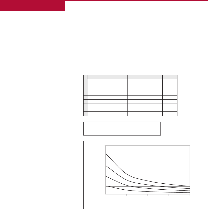
In Equation (4.99) the term A



2 1



multiplied by 100 is the

percent extra area required for the fouled surface compared with the

clean surface. In the following example, we will use the previous

derived relations to develop a graph of percent increase in area

required to compensate for fouling for different values of overall

heat transfer coefficients.

Example 4.17

Using a spreadsheet, develop a chart that shows the relationship between

the total fouling resistance as a function of overall heat transfer coeffi-

cients of 1000 to 5000 W/m

K for cleanliness factors of 0.8, 0.85, 0.9, 0.95.

Also, develop a chart that demonstrates the increase in surface area

required for fouling resistances of 0.0001, 0.001, 0.01, and 0.05 m

K/W for

an overall heat transfer coefficient varying from 1 to 10,000 W/m

Given

Part (a)

Overall heat transfer coefficient 5 1000, 2000, 3000, 4000 and 5000 W/m

Cleanliness factor 5 0.8, 0.85, 0.9, 0.95

Cleanliness Factor

Overall Heat

Transfer

Coefficient

0.80 0.85 0.90 0.95

1000 2.50 1.76 1.11 0.53

2000 1.25 0.88 0.56 0.26

3000 0.83 0.59 0.37 0.18

4000 0.63 0.44 0.28 0.13

5000

ABCDE

7 0.50 0.35 0.22 0.11

0.00

0.50

1.00

1.50

2.00

2.50

3.00

1000 2000 3000 4000 5000

Overall heat transfer coefficient (W/m

Total fouling resistance,

(10

K/W)

0.90

0.80

0.85

0.95

1) Enter values as shown in cells A3:A7 and B2:E2

2) Enter(1/$A3)*(1/B$2-1)*10000 in cell B3 and

copy in cells B4:B7 and C3:E7

■ Figure E4.14 Total fouling resistance as a

function of overall heat transfer coefficient for

different cleanliness factors.

328 CHAPTER 4 Heat Transfer in Food Processing

Part (b)

Fouling resistance 5 0.0001, 0.001, 0.01 and 0.05 m

K/W

Overall heat transfer coefficient 5 1, 10, 100, 1000, 10,000 W/m

Approach

We will develop two spreadsheets using Excelt. First, we will calculate the

fouling resistance for Part (a) and the required increase in surface area for

Part (b). Then we will create a plot from the calculated data.

Solution

The first spreadsheet is developed using Equation (4.95) for the fouling resis-

tance R

as a function of the overall heat transfer coefficient for a clean pipe.

The second spreadsheet is developed using Equation (4.99), and we will plot

2 1



3 100 against overall heat transfer coefficient on a log-log scale. As

we observe, from Figure E4.14, as the cleanliness factor decreases, the fouling

resistance increases for the same value of clean-pipe overall heat transfer

coefficient. This effect is more pronounced at low values of overall heat

transfer coefficient. Similarly, from Figure E4.15, for a small increase in the

100

1 10 100 1000 10000

Overall heat transfer coefficient (W/m

Increase in surface area due

to fouling (%)

0.0001

0.001

0.01

 0.05

1) Enter values as shown in cells A3:A7 and B2:E2

2) Enter  $A3*B$2*100 in cell B3 and

paste in cells B4:B7 and C3:E7

Fouling resistance (m

K/W)

Overall Heat

Transfer

Coefficient

0.05

10 50

100 500

1000 5000

10000

0.0001

0.01

0.1

100

0.01

100

1000

10000

0.001

0.1

100

1000 50000

ABCDE

■ Figure E4.15 Increase in surface area due to

fouling.

3294.4 Steady-S tate Heat Transfer

resistance factor, for the same overall heat transfer coefficient, a much larger

surface area is required. These graphs show that the resistance due to fouling

has a substantial effect on heat transfer, and larger surface areas are required

with increasing fouling.

4.4.7 Design of a Tubular Heat Exchanger

In Section 4.1, we examined a variety of heat exchange equipment

used in the food process industry. Recall that a number of different

geometrical configurations are used in the design of heat exchange

equipment, such as tubular, plate, and scraped surface heat exchan-

gers. The primary objective in using a heat exchanger is to transfer

thermal energy from one fluid to another. In this section we will

develop calculations necessary to design a tubular heat exchanger.

One of the key objectives in calculations involving a heat exchanger

is to determine the required heat transfer area for a given application.

We will use the following assumptions:

1. Heat transfer is under steady-state conditions.

2. The overall heat-transfer coefficient is constant throughout the

length of pipe.

3. There is no axial conduction of heat in the metal pipe.

4. The heat exchanger is well insulated. The heat exchange is

between the two liquid streams flowing in the heat exchanger.

There is negligible heat loss to the surroundings.

Recall from Chapter 1 that change in heat energy in a fluid stream, if

its temperature changes from T

to T

, is expressed as:

q 5

ðT

2 T

Þð4:100Þ

where

m is mass flow rate of a fluid (kg/s), c

is specific heat of a

fluid (kJ/[kg 8C]), and the temperature change of a fluid is from

some inlet temperature T

to an exit temperature T

Consider a tubular heat exchanger, as shown in

Figure 4.28. A hot

fluid, H, enters the heat exchanger at location (1) and it flows through

the inner pipe, exiting at location (2). Its temperature decreases from

H,inlet

to T

H,exit

. The second fluid, C, is a cold fluid that enters the

annular space between the outer and inner pipes of the tubular heat

exchanger at location (1) and exits at location (2). Its temperature

increases from T

C,inlet

to T

C,exit

. The outer pipe of the heat exchanger is

330 CHAPTER 4 Heat Transfer in Food Processing

covered with an insulation to prevent any heat exchange with the sur-

roundings. Because the heat transfer occurs only between fluids H and

C, the decrease in the heat energy of fluid H must equal the increase in

the energy of fluid C. Therefore, conducting an energy balance, the

rate of heat transfer between the fluids is:

q 5

ðT

H,inlet

2 T

H,exit

Þ5

ðT

C,exit

2 T

C,inlet

Þð4:101Þ

where c

is the specific heat of the hot fluid (kJ/[kg 8C]), c

is the

specific heat of the cold fluid (kJ/[kg 8C]),

is the mass flow

rate of the hot fluid (kg/s), and

is the mass flow rate of the cold

fluid (kg/s).

Equation (4.101) is useful if we are interested in determining the

inlet and exit temperatures of the two fluid streams. Furthermore, we

may use this equation to determine the mass flow rate of either fluid

stream, provided all other conditions are known. But, this equation

does not provide us with any information about the size of the heat

exchanger required for accomplishing a desired rate of heat transfer,

and we cannot use it to determine how much thermal resistance to

heat transfer exists between the two fluid streams. For those ques-

tions, we need to determine heat transfer perpendicular to the flow

of the fluid streams, as discussed in the following.

Fluid H Fluid H

Fluid C

Insulation

Temperature

Length or Area

H,inlet

C,inlet

H,exit

C,exit

■ Figure 4.28 A concurrent flow heat

exchanger and temperature plots.

3314.4 Steady-S tate Heat Transfer

Consider a thin slice of the heat exchanger, as shown in Figure 4.28.

We want to determine the rate of heat transfer from fluid H to C, per-

pendicular to the direction of the fluid streams. For this thin slice of

the heat exchanger, the rate of heat transfer, dq, from fluid H to fluid

C may be expressed as:

dq 5 U ΔT dA ð4:102Þ

where ΔT is the temperature difference between fluid H and fluid

C. Note that this temperature difference, ΔT, varies from location

(1) to (2) of the heat exchanger. At the inlet of the fluid streams,

location (1), the temperature difference, ΔT, is T

H,inlet

T

C,inlet

and

on the exit side, location (2), it is T

H,exit

 T

C,exit

(Fig. 4.28). To

solve Equation (4.102) we can substitute only one value of ΔT, or

its average value that represents the temperature gradient perpendic-

ular to the direction of the flow. Although it may be tempting to

take an arithmetic average of the two ΔT values from locations (1)

and (2), the arithmetic average value will be incorrect because, as

seen in Figure 4.28, the temperature plots are nonlinear. Therefore,

we will develop the following mathematical analysis to determine a

value of ΔT that will correctly identify the “average” temperature

difference between the fluids H and C as they flow through the

heat exchanger.

The temperature difference, ΔT, between the two fluids H and C is

ΔT 5 T

2 T

ð4:103Þ

where T

is the temperature of the hot stream and T

is that of the

cold stream. For a small differential ring element as shown in

Figure 4.28, using energy balance for the hot stream H we get

dq 52

ð4:104Þ

and, for cold stream C in the differential element,

dq 5

ð4:105Þ

Equation (4.104), dT

is a negative quantity; therefore, we added

a negative sign to obtain a positive value for dq. Solving for dT

and

, we obtain

ð4:106Þ

332 CHAPTER 4 Heat Transfer in Food Processing

and

ð4:107Þ

Then, subtracting

Equation (4.107) from Equation (4.106),

2 dT

5 dðT

2 T

Þ52dq



ð4:108Þ

Using

Equations (4.102) and (4.103), and substituting in Equation

(4.108),

dðT

2 T

ðT

2 T

52U



dA ð4:109Þ

Integrating

Equation (4.109) from locations (1) to (2) shown in

Figure 4.28,

ðT

H,exit

2 T

C,exit

ðT

H,inlet

2 T

C,inlet

52UA



ð4:110Þ

Noting that

H,inlet

2 T

C,inlet

5 ΔT

H,exit

2 T

C,exit

5 ΔT

ð4:111Þ

we get

ΔT

52UA



ð4:112Þ

Substituting

Equation (4.101) in Equation (4.112),

ΔT



52UA

H,inlet

2 T

H,exit

C,exit

2 T

C,inlet



ð4:113Þ

Rearranging terms in

Equation (4.113),

ΔT



2 UA

ðT

H,inlet

2 T

C,inlet

Þ2 ðT

H,exit

2 T

C,exit



ð4:114Þ

3334.4 Steady-S tate Heat Transfer

Substituting Equation (4.111) in Equation (4.114), we obtain

ΔT



ðΔT

2 ΔT

Þð4:115Þ

Rearranging terms,

q 5 UA

ΔT

2 ΔT

ΔT



ð4:116Þ

q 5 UAðΔT

Þð4:117Þ

where

ΔT

2 ΔT

ΔT



ð4:118Þ

ΔT

is called the log mean temperature difference (LMTD).

Equation (4.117) is used to design a heat exchanger and determine

its area and the overall resistance to heat transfer, as illustrated in

Examples 4.18 and 4.19.

Example 4.18

A liquid food (specific heat 5 4.0 kJ/[kg 8C]) flows in the inner pipe of a

double-pipe heat exchanger. The liquid food enters the heat exchanger at

208C and exits at 608C(

Fig. E4.16). The flow rate of the liquid food is

0.5 kg/s. In the annular section, hot water at 908C enters the heat

exchanger and flows countercurrently at a flow rate of 1 kg/s. The average

specific heat of water is 4.18 kJ/(kg 8C). Assume steady-state conditions.

1. Calculate the exit temperature of water.

2. Calculate log-mean temperature difference.

3. If the average overall heat transfer coefficient is 2000 W/(m

8C)

and the diameter of the inner pipe is 5 cm, calculate the length of

the heat exchanger.

4. Repeat these calculations for parallel-flow configuration.

Given

Liquid food:

Exit temperature 5 608C

Inlet temperature 5 208C

Length (m)

Temperature (°C)

90°C

60°C

20°C

■ Figure E4.16 A countercurrent flow heat

exchanger with unknown exit temperatures.

334 CHAPTER 4 Heat Transfer in Food Processing

Specific heat 5 4.0 kJ/(kg 8C)

Flow rate 5 0.5 kg/s

Water:

Inlet temperature 5 908C

Specific heat 5 4.18 kJ/(kg 8C)

Flow rate 5 1.0 kg/s

Heat exchanger:

Diameter of inner pipe 5 5cm

Flow 5 countercurrent

Approach

We will first calculate the exit temperature of hot water by using a simple

heat balance equation. Then we will compute log-mean temperature differ-

ence. The length of the heat exchanger will be determined from

Equation

(4.117). The solution will be repeated for parallel-flow configuration to obtain

a new value for log-mean temperature difference and length of the heat

exchanger.

Solution

1. Using a simple heat balance,

q 5

ΔT

5 (0:5kg=s)(4kJ=[kg 8C])(608C 2 20 8C)

5 (1 kg=s)(4:18 kJ=[kg 8C])(908C 2 T

8C)

5 70:98C

2. The exit temperature of water is 70.98C.

3. From

Equation (4.118)

(ΔT)

Δ(T)

2 Δ(T)

Δ(T)

(70:9 2 20) 2 (902 60)

50:9

5 39:58C

4. The log-mean temperature difference is 39.58C.

5. From

Equation (4.117),

q 5 UA(ΔT)

5 U π D

L(ΔT)

where q, from step (1), is

q 5 (0:5kg=s)(4 kJ=[kg 8C])(608C 2 208C) 5 80 kJ=s

3354.4 Steady-S tate Heat Transfer

Thus,

L 5

(80 kJ=s)(1000 J=kJ)

(π)(0:05 m)(39:58C)(2000 W=[m

8C])

5 6:45 m

6. The length of the heat exchanger, when operated counter-currently, is

6.5 m.

7. For parallel-flow operation, the system diagram will be as shown in

Figure E4.16 .

8. Assuming that for parallel flow the exit temperature will be the same

as for counterflow, T

5 70.98C.

9. Log-mean temperature difference is calculated from

Equation (4.118).

(ΔT)

(90 2 20) 2 (70:9 2 60)

90 2 20

70:9 2 60



5 31:88C

10. The log-mean temperature difference for parallel flow is 31.88C, about

88C less than that for the countercurrent flow arrangement.

11. The length can be computed as in step (5).

L 5

(80 kJ=s)(1000 J=kJ)

(π)(0:05 m)(31:88C)(2000 W=[m

8C])

5 8m

12. The length of the heat exchanger, when operated as parallel flow, is

8 m. This length of heat exchanger is longer by 1.55 m to obtain the

same exit temperature of hot-water stream as for the counterflow

arrangement.

Example 4.19

Steam with 90% quality, at a pressure of 143.27 kPa, is condensing in the

outer annular space of a 5 m-long double-pipe heat exchanger (

Fig. E.17

and E4.18). Liquid food is flowing at a rate of 0.5 kg/s in the inner pipe.

The inner pipe has an inside diameter of 5 cm. The specific heat of the liq-

uid food is 3.9 kJ/(kg 8C). The inlet temperature of the liquid food is 408C

and the exit temperature is 808C.

a. Calculate the average overall heat-transfer coefficient.

b. If the resistance to conductive heat transfer caused by the inner steel

pipe is negligible, and the convective heat-transfer coefficient on the

steam side is very large (approaches infinity), estimate the convective

heat-transfer coefficient for the liquid food in the inside pipe.

Length (m)

Temperature (°C)

90°C

60°C

20°C

70.9°C

■ Figure E4.17 Temperature plots for a

counterflow heat exchanger.

336 CHAPTER 4 Heat Transfer in Food Processing

Given

Steam pressure 5 143.27 kPa

Length 5 5m

Flow rate of liquid 5 0.5 kg/s

Inside diameter 5 0.05 m

Specific heat 5 3.9 kJ/(kg 8C)

Product inlet temperature 5 408C

Product exit temperature 5 808C

Approach

We will obtain steam temperature from Table A.4.2. We also note that steam

quality has no effect on the steam condensation temperature. We will calcu-

late the heat required to raise the liquid food temperature from 40 to 808C.

Next, we will calculate log-mean temperature difference. Then we will obtain

the overall heat-transfer coefficient by equating the heat gain of the liquid

food and heat transfer across the pipe wall, from steam to the liquid food.

Solution

Part (a)

1. From steam table (Table A.4.2), steam temperature 5 1108C.

q 5

ΔT

5 (0:5kg=s)(3:9kJ=[kg 8C])(1000 J=kJ)(808C 2 408C)

5 78, 000 J=s

q 5 UA(ΔT)

ΔT

(ΔT)

(110 2 40) 2 (110 2 80)



110 2 40

110 2 80



5 47:28C

and

A 5 π(0:05)(5) 5 0:785 m

U 5

ΔT

A(ΔT)

(78,800 J=s)

(0:785 m

)(47:28C)

5 2105 W=(m

8C)

5. Overall heat-transfer coefficient 5 2105 W/(m

8C)

Length (m)

Temperature (°C)

110°C

80°C

40°C

110°C

■ Figure E4.18 Temperature plots for a

parallel-flow heat exchanger.

3374.4 Steady-S tate Heat Transfer

Part (b)

The overall heat-transfer equation may be written as follows:



2π kL

The second term on the right-hand side of the above equation is zero, since

the resistance offered by steel to conductive heat transfer is considered negli-

gible. Likewise, the third term is zero, because the convective heat-transfer

coefficient on the steam side is very large.

Therefore,

5 h

5 2105 W=(m

8C)

4.4.8 The Effectiveness- NTU Method for Designing

Heat Exchangers

In the preceding section, we used the log-mean-temperature-

difference (LMTD) approach to design a heat exchanger. The LMTD

approach works well when we are designing a new heat exchanger,

where the temperatures of the fluid streams at the inlet and exit are

known and we are interested in determining the size of the heat

exchanger (in terms of the heat transfer area, length, and diameter of

the pipe). However, in other situations when the size of the heat

exchanger, and the inlet temperatures of the product and heating/

cooling streams are known but the exit temperatures of the two

streams are unknown, the LMTD approach can be used but the solu-

tion requires iterative procedures and becomes tedious. For this pur-

pose, another calculation technique called the effectiveness-NTU

method is easier to use. This method involves three dimensionless

quantities, namely the heat capacity rate ratio, heat exchanger effec-

tiveness, and number of transfer units (NTU).

4.4.8.1 Heat Capacity Rate Ratio, C*

A heat capacity rate of a liquid stream is obtained as a product of the

mass flow rate and specific heat capacity. Thus, for the hot and cold

338 CHAPTER 4 Heat Transfer in Food Processing

streams the heat capacity rates are, respectively:

ð4:119Þ

ð4:120Þ

These two quantities are evaluated using the given data in a problem;

the smaller of the two quantities is called C

min

and the larger C

max

The heat capacity rate ratio, C*, is defined as



min

max

ð4:121Þ

4.4.8.2 Heat Exchanger Effectiveness, ε

The heat exchanger effectiveness is a ratio of the actual rate of heat

transfer accomplished and the maximum attainable rate of heat

transfer for a given heat exchanger. The heat exchanger effectiveness,

, is defined as

actual

max

ð4:122Þ

The actual rate of heat transfer can be determined for both hot and

cold streams as

actual

5 C

ðT

H,inlet

2 T

H,exit

Þ5 C

ðT

C,exit

2 T

C,inlet

Þð4:123Þ

And, the maximum rate of attainable heat transfer is obtained by

observing that in any heat exchanger the maximum possible temper-

ature difference is between the temperatures of hot and cold streams

at the inlet. This temperature difference is multiplied with the mini-

mum heat capacity rate, C

min

, to obtain q

max

5 C

min

ðT

H,inlet

2 T

C,inlet

Þð4:124Þ

Thus, from

Equation (4.122),

actual

5 ε

max

5 ε

min

ðT

H,inlet

2 T

C,inlet

Þð4:125Þ

3394.4 Steady-S tate Heat Transfer

4.4.8.3 Number of Transfer Units, NTU

The number of transfer units provides a measure of the heat transfer

surface area for a given overall heat transfer coefficient and minimum

heat capacity rate. It is expressed as

NTU 5

min

ð4:126Þ

where A is the heat transfer area (m

), U is the overall heat transfer

coefficient (W/m

8C) based on the selected area (see Section 4.4.5),

and C

min

is the minimum heat capacity rate (W/8C).

Relationships between NTU and effectiveness can be obtained for dif-

ferent types of heat exchangers with prescribed flow conditions (such

as counterflow or concurrent flow). These relationships include the

heat capacity rate ratios. Some of these relationships for commonly

used heat exchangers are shown in

Tables 4.4 and 4.5.InTable 4.4,

the exchanger effectiveness is given in terms of NTU, and in

Table 4.5, the NTU values are given as a function of the exchanger

effectiveness. The steps involved in using the effectiveness-NTU

method are illustrated in the following example.

Table 4.4 Effectiveness-NTU Relations for Heat Exchangers

Type of heat

exchanger Effectiveness relation

Double pipe

Concurrent flow

1 2 exp½2NTUð1 1 C



Þ

1 1 C

Double pipe

Countercurrent flow

1 2 exp½2NTUð1 1 C



Þ

1 2 C



exp½2NTUð1 2 C



Þ

Shell and tube:

One-shell pass

2, 4, 6... tube passes

1 1 C



ﬃﬃﬃﬃﬃﬃﬃﬃﬃﬃﬃﬃﬃﬃﬃ

1 1 C

2

1 1 exp 2NTU

ﬃﬃﬃﬃﬃﬃﬃﬃﬃﬃﬃﬃﬃﬃﬃ

1 1 C

2

1 2 exp 2NTU

ﬃﬃﬃﬃﬃﬃﬃﬃﬃﬃﬃﬃﬃﬃﬃ

1 1 C

2

Plate heat exchanger

exp½ð1 2 C



Þ3 NTU 2 1

exp½ð1 2 C



Þ3 NTU 2 C



All heat exchangers,

C* 5 0

5 1 2 expð2NTUÞ

340 CHAPTER 4 Heat Transfer in Food Processing

Example 4.20

We will use some of the data from Example 4.18 to show the use of the

effectiveness-NTU method in solving problems when both exit tempera-

tures are unknown. A liquid food (specific heat 5 4.0 kJ/[kg 8C]) flows in

the inner pipe of a double-pipe heat exchanger. The liquid food enters the

heat exchanger at 208C. The flow rate of the liquid food is 0.5 kg/s. In the

annular section, hot water at 908C enters the heat exchanger and flows in

countercurrent direction at a flow rate of 1 kg/s. The average specific heat

of water is 4.18 kJ/(kg 8C). The average overall heat transfer coefficient

based on the inside area is 2000 W/(m

8C), and the diameter of the inner

pipe is 5 cm and length is 6.45 m. Assume steady state conditions.

Calculate the exit temperature of liquid food and water.

Given

Liquid food:

Inlet temperature 5 208C

Specific heat 5 4.0 kJ/(kg 8C)

Flow rate 5 0.5 kg/s

Table 4.5 NTU-Effectiveness Relations for Heat Exchangers

Type of heat exchanger NTU relation

Double pipe

Concurrent flow

NTU 52

ln½1 2 ε

ð1 1 C



Þ

1 1 C



Double pipe

Countercurrent flow

NTU 5

1 2 C



1 2 C



1 2 ε

ðC



,1Þ

NTU 5

1 2 ε

ðC



5 1Þ

Shell and tube:

One-shell pass

2, 4, 6... tube passes

NTU 5

ﬃﬃﬃﬃﬃﬃﬃﬃﬃﬃﬃﬃﬃﬃﬃ

1 1 C

2

2 2 ε

1 1 C



ﬃﬃﬃﬃﬃﬃﬃﬃﬃﬃﬃﬃﬃﬃﬃ

1 1 C

2

2 2 ε

1 1 C



ﬃﬃﬃﬃﬃﬃﬃﬃﬃﬃﬃﬃﬃﬃﬃ

1 1 C

2

Plate heat exchanger

NTU 5

ð1 2 C



ð1 2 ε



ð1 2 C



All heat exchangers, C* 5 0 NTU 52lnð1 2 ε

3414.4 Steady-S tate Heat Transfer

Water:

Inlet temperature 5 908C

Specific heat 5 4.18 kJ/(kg 8C)

Flow rate 5 1.0 kg/s

Heat exchanger:

Diameter of inner pipe 5 5cm

Length of inner pipe 5 6.45 m

Overall heat transfer coefficient 5 2000 W/m

Flow 5 countercurrent

Approach

Since exit temperatures of both streams are unknown (Fig. E4.19), we will use

the effectiveness-NTU method. We will first calculate the maximum and mini-

mum heat capacity rates. The two heat capacity rates will be used to calcu-

late the heat capacity rate ratio, C*. Next, we will obtain NTU from the given

overall heat transfer coefficient, heat exchanger area, and the calculated

value of C

min

. Using the calculated value of NTU, we will use an appropriate

table to determine the exchanger effectiveness. The definition of the

exchanger effectiveness will be used to determine q

actual

, and the unknown

temperatures, T

H,exit

and T

L,exit

Solution

1. The heat capacity rates for the hot water and liquid food are,

respectively,

5 (1:0kg=s)ð4:18 kJ=[kg 8C])

5 4:18 kW=8C

5 (0:5kg=s)ð4kJ=[kg 8C])

5 2kW=8C

Therefore, using the smaller value of C between the above calculated

values C

and C

min

5 2kW=8C

Then, C* is obtained as



4:18

5 0:4785

Length (m)

Temperature (°C)

90°C

20°C

■ Figure E4.19 Temperature plots for a

double-pipe heat exchanger.

342 CHAPTER 4 Heat Transfer in Food Processing

2. The NTU value is obtained from Equation (4.126) as

NTU 5

min

(2000 W=m

8C)(π)(0:05 m)(6:45m)

(2 kW=8C)(1000 W=kW)

NTU 5 1:0132

3. From

Table 4.4 we select an expression for ε

for tubular heat

exchanger, for counterflow, and substitute known terms as

1 2 e

(21:0132(120:4785))

1 2 0:4785e

(21:0132(1204785))

5 0:5717

According to

Equation (4.124)

max

5 (2kW=8C)(90 2 20)(8C) 5 140 kW

Since ε

actual

max

actual

5 0:5717 3 140(kW) 5 80:038 kW

For hot water stream:

actual

5 4:18(kW=8C) 3 (90 2 T

H,exit

)(8C) 5 80:038 kW

H,exit

5 90 2 19:15 5 70:858C

Similarly, for liquid food stream:

actual

5 2(kW=8C) 3 (T

L,exit

2 20)(8C) 5 80 :038 kW

L,exit

5 40:019 1 20 5 608C

The calculated exit temperatures of hot water and product streams are

70.858C and 608C, respectively. These values are comparable to those

given in Example 4.18.

4.4.9 Design of a Plate Heat Exchanger

As discussed in Section 4.1.1, plate heat exchangers are commonly

used in the food industry. The design of a plate heat exchanger

requires certain relationships that are often unique to the plates used

in the heat exchanger. Some of the required information for design

3434.4 Steady-S tate Heat Transfer

purposes is closely guarded by the equipment manufacturers and is

not readily available. We will consider a general design approach

with some of the key relationships required in designing plate heat

exchangers. First, it is important to understand the type of flow pat-

tern present inside a plate heat exchanger.

Figure 4.2 shows an arrangement of plates with two liquid streams,

product and heating/cooling medium, entering and exiting through

their respective ports. The assembly of a plate heat exchanger

involves placing the required number of plates in a frame and tight-

ening the end bolts so that a fixed gap space is created between the

plates. The gaps between the plates create channels through which

the fluid streams flow. The fluid streams enter and exit through the

port holes (Fig. 4.2b).

Each plate contains a gasket that helps orient the direction of the

flow stream through the channel. The assembly of plates with gaskets

is done in such a manner that it allows the product stream to move

in one channel while the heating/cooling stream moves in the neigh-

boring channel. Thus, the flow of product and heating/cooling

streams alternates through the channels and they never come into

direct contact (

Fig. 4.2).

The heat exchange between the two liquid streams in a plate heat

exchanger is across the plates, normal to the direction of the flow.

Therefore, the plates are made as thin as possible to minimize resis-

tance to heat transfer while maintaining the physical integrity of the

plates. The plates are corrugated with a pattern that promotes turbu-

lence in the liquid stream. Several types of patterns are used for the

corrugations stamped on the plates, the most common one being a

herringbone type design called the Chevron design (

Fig. 4.3). The

plates used in food processing applications are made of stainless steel

(ANSI 316), although the thermal conductivity of stainless steel is

not as high as other metals that are used in nonfood applications. In

the past, the material used for gaskets did not permit use of high

temperatures. However, new heat-resistant materials for gaskets have

considerably extended the use of plate heat exchangers for high-

temperature applications.

To determine the rate of heat transfer across the plates, it is necessary

to know the convective heat transfer coefficient on both sides of the

plates. Since the mechanism is forced convection, we use a dimen-

sionless correlation involving Nusselt number, Reynolds number,

and Prandtl number. The dimensionless correlation depends upon

344 CHAPTER 4 Heat Transfer in Food Processing

the design of the corrugations used. An approximate expression

suitable for plate heat exchanger is as follows:

5 0:4N

0:64

0:4

ð4:127Þ

To evaluate the Reynolds number, it is necessary to determine the

velocity of the liquid stream in the channel. This determination is

complex because of the corrugations. We will consider a simplified

method to estimate the fluid velocity.

In a plate heat exchanger, the two end plates do not take part in heat

transfer. Thus, the number of “thermal plates” involved in heat trans-

fer is obtained by subtracting two from the total number of plates in

a heat exchanger.

The flow rate of a liquid stream through each channel is obtained as

N 1 1



ð4:128Þ

and

N 1 1

ð4:129Þ

where

and

are the total mass flow rates of the heating/cooling

stream and the product stream (kg/s), respectively;

and

are

the channel flow rates for heating/cooling stream and product stream

(kg/s), respectively; and N is the total number of thermal plates.

The cross-sectional area of a channel between two adjacent plates is

obtained as,

5 bw ð4:130Þ

where b is the gap between two adjacent plates and w is the width of

the plate.

The velocities of the two streams are

ð4:131Þ

ð4:132Þ

3454.4 Steady-S tate Heat Transfer

The equivalent diameter (or the hydraulic diameter), D

, is calculated

from the following expression:

4 3 channel free-flow area for fluid stream

wetted perimeter for the fluid

ð4:133Þ

For simplicity, we use the projected area (disregarding the corruga-

tions) to determine the wetted perimeter as

wetted perimeter for the fluid 5 2ðb 1 wÞð4:134Þ

Channel free-flow area 5 bw ð4:135Þ

Then,

4bw

2ðb 1 wÞ

ð4:136Þ

Since in a plate heat exchanger, b{w, we may neglect b in the

denominator to obtain,

5 2 3 b ð4:137Þ

The Reynolds number for each stream is obtained as

Product stream:

Re,P

ð4:138Þ

Heating/cooling stream:

Re,H

ð4:139Þ

Knowing the Reynolds number, the Nusselt number is calculated for

each stream using

Equation (4.127). The heat transfer coefficient is

obtained as

3 k

ð4:140Þ

3 k

ð4:141Þ

346 CHAPTER 4 Heat Transfer in Food Processing

where k

and k

are the thermal conductivities of the product and

heating/cooling streams, (W/m 8C), respectively.

The overall heat transfer coefficient is determined from the two

values of the convective heat transfer coefficients, assuming that the

conductive resistance of the thin metal plate is negligible,

ð4:142Þ

Once the overall heat transfer coefficient is obtained using

Equation

(4.142), the remaining computations for the design of the plate heat

exchanger are done using the effectiveness-NTU method similar to

the procedure described in Section 4.4.7.2. For a plate heat

exchanger, the relevant expressions between NTU and effectiveness

are given in Tables 4.4 and 4.5. The calculation procedure for design-

ing a plate heat exchanger is illustrated in the following example.

Example 4.21

A c ounterflow plate h eat exc hanger is b eing us ed to heat apple juice

with hot water. The heat exchanger contains 51 plates. Each plate is

1.2 m high and 0.8 m wide. The gap between the plates is 4 mm. The

heating characteristics for this heat ex changer have been pre viously

determined to follow the following relationship, N

5 0:4N

0:64

0:4

.Hot

water enters the heat exchanger at 958C at a rate of 15 kg/s and apple

juice enters at 158C at a rate of 10 kg/s. It is assumed that the physical

properties of water and apple juice are the sa me. The properties of water

at 558C are density 5 985.7 kg/m

, specific heat 5 4179 J/kgK, thermal

cond uctivity 5 0.652 W/m 8C, dynamic viscosity 5 509.946 3 10

Prandtl Number 5 3.27. Calculate the exit temperatures of water and

apple juice.

Given

Number of plates 5 51

Plate height 5 1.2 m

Plate width 5 0.8 m

Gap between plates 5 4mm5 0.004 m

Inlet temperature of hot water 5 958C

Mass flow rate of hot water 5 15 kg/s

Inlet temperature of apple juice 5 158C

Mass flow rate of apple juice 5 10 kg/s

Properties of water at (95 1 15)/2 5 558C from Table A.4.1

Density 5 985.7 kg/m

Specific heat 5 4.179 kJ/kgK

3474.4 Steady-S tate Heat Transfer

Thermal conductivity 5 0.652 W/m 8C

Viscosity 5 509.946 3 10

Ns/m

Prandtl number 5 3.27

Approach

We will assume that the heat exchanger is operating under steady state condi-

tions. First, we will determine the channel velocity of each fluid stream using

the given flow rates and gap dimensions. Next, we will determine the Reynolds

number, and using the dimensionless correlation, we will calculate Nusselt

number and convective heat transfer coefficient. The convective heat transfer

coefficients from both sides of a plate will be used to determine the overall heat

transfer coefficient. Once the overall heat transfer coefficient is known, then we

will use the effectiveness-NTU method to determine the exit temperatures of

each stream.

Solution

Heat transfer coefficient on the hot water side:

1. Equivalent diameter for the channel created between the plates is

5 2 3 b 5 2 3 0:004 5 0:008 m

2. Flow rate of hot water in each channel:

Total number of plates 5 51. Since the two end plates do not take

part in heat exchange, the number of thermal plates 5 49. Then

2 3 15

(491 1)

5 0:60 kg=s

3. The cross-sectional area of each channel is

5 0:004 3 0:8 5 0:0032 m

4. Velocity of hot water in each channel is

0:60 (kg=s)

985:7(kg=m

) 3 0:0032 (m

)

5 0:19 m=s

5. Reynolds number:

985:7 3 0:19 3 0:008

509:946 3 10

5 2941

6. Nusselt number:

5 0:4 3 2941

0:64

3 3:27

0:4

5 106:6

348 CHAPTER 4 Heat Transfer in Food Processing

Then, heat transfer coefficient on the hot water side is

106:6 3 0:652

0:008

5 8,688 W=m

Heat transfer coefficient on the apple juice side:

7. The flow rate of apple juice in each channel is

2 3 10

(49 1 1)

5 0:4kg=s

8. The velocity of apple juice in each channel is

0:4 ðkg=s)

985:7(kg=m

) 3 0:0032 (m

)

5 0:127 m=s

9. The Reynolds number is

985:7 3 0:127 3 0:008

509:946 3 10

5 1961

10. The Nusselt number is

5 0:4 3 1961

0:64

3 3:27

0:4

5 82:2

11. Convective heat transfer coefficient on the apple juice side is

82:2 3 0: 652

0:008

5 6702 W=m

12. The overall heat transfer coefficient, U, is

8688

6702

U 5 3784 W=m

13. The total area of the heat exchanger is

5 49 3 1:2 3 0:8 5 47:04 m

14. NTU for the heat exchanger is

NTU 5

3784 3 47:04

10 3 4179

5 4:259

15. The capacity rate ratio is



5 0:67

3494.4 Steady-S tate Heat Transfer

16. The exchanger effectiveness is obtained from the relationship given in

Table 4.4 as

exp[(1 2 0:67) 3 4:259] 2 1

exp[(1 2 0:67) 3 4:259] 2 0:67

5 0:9

17. The exit temperature of apple juice is determined by noting that

juice

5 C

min

, or

actual

max

5 0:9 5

juice

2 15)

min

(952 15)

2 15)

(95 2 15)

Then, T

5 878C

18. The exit temperature of hot water is determined as

0:9 5

water

(95 2 T

)

min

(95 2 15)

5 1:5

(95 2 T

)

(95 2 15)

or, T

5 478C

In the given counter flow plate heat exchanger operating under stea-

dy state conditions, the hot water stream will exit at 478C and the

apple juice will be heated to 878C.

4.4.10 Importance of Surface Characteristics in

Radiative Heat Transfer

All materials in the universe emit radiation of an electromagnetic

nature based on their surface temperature. At a temperature of 0K,

the emission of radiation ceases. The characteristics of the radiation

are also dependent on temperature. As temperature increases, the

wavelength decreases. For example, radiation emitted by the sun is

shortwave compared with the longwave radiation emitted by the sur-

face of a hot coffee mug.

When radiation of a given wavelength, as shown in

Figure 4.29, is

incident on an object, some of the incident radiation is reflected,

some transmitted, and some absorbed. The following expression

holds true:

φ 1 χ 1 ψ 5 1 ð4:143Þ

where φ is absorptivity, χ is reflectivity, and ψ is transmissivity. The

absorbed radiation will result in an increase of temperature.

Reflected

Absorbed

Transmitted

Emitted

Incident

■ Figure 4.29 Radiant energy incident on a

semi-opaque object.

350 CHAPTER 4 Heat Transfer in Food Processing

To compare the absorption of radiation for different materials , an

ideal reference called a blackbody is used. For a blackbody, the

absorptivity value is 1.0. Note that nothing in the universe is a true

blackbody; even lampblack has φ 5 0.99 and χ 5 0.01. Regardless,

blackbody is a useful concept for comparing radiative properties of

different materials.

The absolute magnitudes of φ, χ, and ψ depend on the nature of the

incident radiation. Thus, a brick wall of a house is opaque to visible

light but transparent to radio waves.

Energy emitted (also called radiated) and energy reflected must be

clearly distinguished. These are quite different terms. A material,

depending on its surface absorptivity value, will reflect some of the

incident radiation. In addition, based on its own temperature, it will

emit radiation, as shown in

Figure 4.29. The amount of radiation

emitted can be computed from Equation (4.20).

Kirchoff’s law states that the emissivity of a body is equal to its

absorptivity for the same wavelength. Thus, mathematically,

ε 5 φ ð4:144Þ

This identity is discussed in Example 4.22.

Example 4.22

Compare the selection of white paint versus black paint for painting the

rooftop of a warehouse. The objective is to allow minimum heat gain from

the sun during summer.

Given

White paint from Table A.3.3:

shortwave

5 0.18

longwave

5 0.95

Black paint from Table A.3.3:

shortwave

5 0.97

longwave

5 0.96

Approach

From the emissivity values, we will examine the use of white or black paint

for both short- and longwave radiation.

3514.4 Steady-S tate Heat Transfer

Solution

1. White paint: ε

shortwave

5 0.18, therefore from Kirchoff’s law

shortwave

5 0.18, so χ

shortwave

5 1 2 0.18, assuming ψ 5 0, thus

shortwave

5 0.82. Thus, of the total shortwave radiation incident on the

rooftop, 18% is absorbed and 82% reflected.

2. White paint, ε

longwave

5 0.95. The white-painted surface , in terms of

longwave radiation, emits 95% of radiation emitted by a blackbody.

3. Black paint: ε

shortwave

5 0.97, therefore using Kirchoff’sLaw

shortwave

5 0.97. Thus, of the total shortwave radiation incident on the

rooftop, 97% of radiation incident on it is absorbed and 3% is reflected.

4. Black paint: ε

longwave

5 0.96. The black-painted surface, in terms of

longwave radiation, emits 96% of radiation emitted by a blackbody.

5. White paint should be selected, as it absorbs only 18% shortwave (solar)

radiation compared to 97% by black paint. Both black and white paint

are similar in emitting longwave radiation to the surroundings.

4.4.11 Radiative Heat Transfer between Two Objects

The transfer of heat by radiation between two surfaces is dependent

on the emissivity of the radiating surface and the absorptivity of that

same surface. The expression normally used to describe this type of

heat transfer is as follows:

122

5 Aσðε

2 φ

122

Þð4:145Þ

where ε

is the emissivity of the radiating surface at temperature T

and φ

12

is the absorptivity of the surface for radiation emitted at

temperature T

Although the basic expression describing radiative heat transfer is given

Equations (4.20) and (4.145), one of the important factors requiring

attention is the shape of the object. The shape factor accounts for the

fraction of the radiation emitted by the high-temperature surface that is

not absorbed by the low-temperature surface. For example, Equation

(4.145) assumes that all radiation emitted at temperature T

absorbed by the surface at temperature T

. If both the surfaces are

blackbodies, then the expression describing heat transfer and incorpo-

rating the shape factor would be as follows:

122

5 σF

122

ðT

2 T

Þð4:146Þ

where F

12

is the shape factor, and it physically represents the frac-

tion of the total radiation leaving the surface A

that is intercepted by

352 CHAPTER 4 Heat Transfer in Food Processing

the surface A

. The values of shape factors have been tabulated and

presented in the form of curves of the type shown in

Figures 4.30

and 4.31. In the first case, the shape factors deal only with adjacent

rectangles, which are in perpendicular planes. Figure 4.31 can be uti-

lized for various shapes, including disks, squares, and rectangles.

Equation (4.146) does not account for nonblackbodies, and

Equation (4.20) does not account for the shape factor; therefore, an

expression that combines the two must be used. Such an expression

would be

122

5 σA

122

ðT

2 T

Þð4:147Þ

0.50

0.45

0.40

0.35

0.30

0.25

0.20

Factor (F

1–2

)

0.15

0.10

0.05

0 0.5 1.0 1.5 2.0 2.5 3.0

8.0

4.0

3.0

2.0

1.6

1.4

1.2

0.9

0.7

0.5

0.3

0.2

Y  6.0

Dimension ratio (Z )

Scale changes here

Asymp-

totes

3.5 4.0 5 6 7 8 9 10

Y  1.0

2.5

Y  0.1

0.4

■ Figure 4.30 Shape factors for adjacent rectangles in perpendicular planes. Y (dimension ratio) 5 y/x; Z 5 z/x. (Adapted from Hottel, 1930)

3534.4 Steady-S tate Heat Transfer

where the ξ

12

factor accounts for both shape and emissivity. This

factor can be evaluated by the following expression:

122

2 1



2 1



ð4:148Þ

Equations (4.147) and (4.148) can be used to compute the net radi-

ant heat transfer between two gray bodies in the presence of radiating

surfaces at uniform temperatures.

Example 4.23

Compute the radiative heat transfer received by a rectangular product mov-

ing through a radiation-type heater (

Fig. E4.20). The radiation source is one

vertical wall of a heater and is held at a constant temperature of 2008C while

the product is moving perpendicular to the radiation source. The product

temperature is 808C with an emissivity of 0.8. The product dimensions are

15 3 20 cm, and the radiation source is 1 3 5m.

Given

Temperature of heater 5 2008C

Product temperature 5 808C

Emissivity of product 5 0.8

Product dimensions 5 0.15 m 3 0.2 m

Heater dimensions 5 1m3 5m

1.0

0.8

0.6

Factor (F

1–2

)

0.4

0.2

01234

Ratio

Side or diameter

Distance between planes

567

⎞

⎠

⎛

⎝

■ Figure 4.31 Shape factors for equal and

parallel squares, rectangles, and disks: (1) direct

radiation between disks; (2) direct radiation

between squares; (3) total radiation between

squares or disks connected by nonconducting but

reradiating walls. (Adapted from

Hottel, 1930)

354 CHAPTER 4 Heat Transfer in Food Processing

Approach

To compute the ξ

12

factor from Equation (4.148), we will use Figure 4.30, for

objects perpendicular to each other, for F

12

value. Then we will use Equation

(4.147) to calculate radiative heat received by the rectangular product.

Solution

1. To use Equation (4.147), the ξ factor must be computed from Equation

(4.148).

122

2 1



0:03

0:8

2 1



where F

12

must be obtained from Figure 4.30 for z/x 5 5.0 and

y/x 5 0.75.

122

5 0:28

Then

122

(3:57 1 0 1 41:67)

45:24

5 0:0221

2. From

Equation (4.147),

122

5 (5:669 3 10

W=[m

])(0:0221)(5 m

)

3 [(473 K)

2 (353 K)

]

5 216 W

4.5 UNSTEADY-STATE HEAT TRANSFER

Unsteady-state (or transient) heat transfer is that phase of the heating

and cooling process when the temperature changes as a function of

both location and time. By contrast, in steady-state heat transfer, tem-

perature varies only with location. In the initial unsteady-state period,

many important reactions in the food may take place. With thermal

processes, the unsteady-state phase may even dominate the entire pro-

cess; for example, in several pasteurization and food-sterilization pro-

cesses, the unsteady-state period is an important component of the

process. Analysis of temperature variations with time during the

unsteady-state period is essential in designing such a process.

Since temperature is a function of two independent variables, time

and location, the following partial differential equation is the govern-

ing equation for a one-dimensional case:

ρc



ð4:149Þ

Heater

Product

5 m

1 m

15 cm

20 cm

■ Figure E4.20 Radiation heater.

3554.5 Unsteady-State Heat Transfer

where T is temperature (8C), t is time (s), and r is distance from cen-

ter location (m). We can make this equation specific for a particular

geometrical shape using n 5 0 for a slab, n 5 1 for a cylinder, and

n 5 2 for a sphere. The combination of properties k/ρc

is defined as

thermal diffusivity, α. If the rate of heat transfer at the surface of the

object is due to convection, then

r5R

5 hðT

2 T



ð4:150Þ

where h is the convective heat transfer coefficient (W/[m

8C]), T

the temperature of heating or cooling medium far away from the sur-

face (8C), and T

is the temperature at the surface (8C).

The procedure we use to solve the governing equation,

Equation

(4.149), involves the use of advanced mathematics, which is beyond

the scope of this book. Myers (1971) gives the complete derivation

for various types of boundary-value problems encountered in

unsteady-state heat transfer. Due to mathematical complexity, the

analytical solution of Equation (4.149) is possible only for objects of

simplified geometrical shapes, such as a sphere, an infinite cylinder,

or an infinite slab.

An infinite cylinder is a “long” cylinder of radius r, a sphere is of

radius r, an infinite plate is a “large” plane wall of thickness 2z. These

three objects are geometrically and thermally symmetric about their

centerline (for a cylinder), center plane (for a slab), or center point

(for a sphere), as shown in

Figure 4.32.

Consider heating an infinitely long cylindrical object. Initially, the

object is assumed to have a uniform temperature, T

. At time t 5 0,

we place this object in a heating medium maintained at a constant

temperature T

. A constant heat transfer coefficient, h, describes the

convective heat transfer at the surface of the object. Temperature pro-

files at different time intervals inside the object are shown in

Figure 4.33. At time t 5 0, the temperature is uniform at T

. At time,

t 5 t

, the temperature along the wall increases, establishing a temper-

ature gradient within the object that promotes heat conduction. At

time t 5 t

, the temperature at the center is still at T

. However, with

the passage of time, at time t 5 t

, the centerline temperature begins

to increase, and eventually at t 5 t

the temperature of the cylinder

becomes uniform at T

. At this time, the cylinder is in thermal equi-

librium with the surrounding medium, and heat transfer ceases. Note

that there is no heat transfer from the axial ends of the cylinder.

356 CHAPTER 4 Heat Transfer in Food Processing

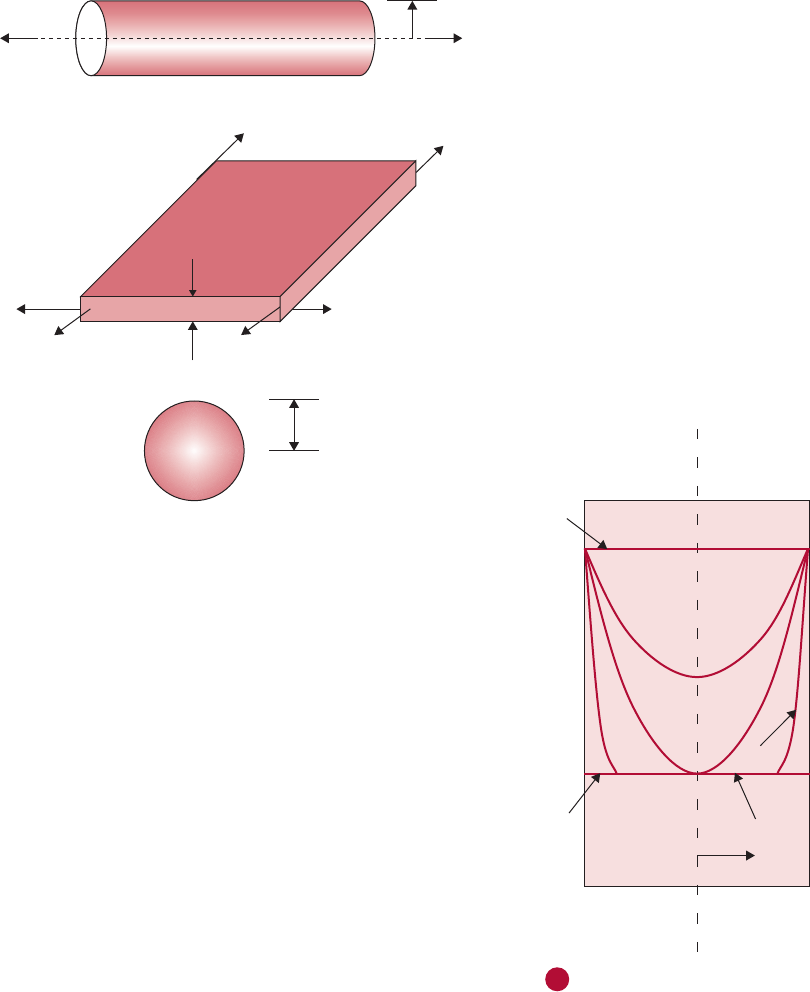
Because the cylinder is infinitely long , the implication of “infinite”

length in this case is that the heat transfer is only in the radial direc-

tion and not axial. Similarly, for an infinite slab of thickness, 2z, the

heat transfer is only from the two faces around the thickness 2z of

the slab. The slab extends to infinity along the other four faces, and

no heat transfer takes place through those sides. We will explore

these concepts in greater detail in the following sections.

4.5.1 Importance of External versus Internal

Resistance to Heat Transfer

In transient heat transfer analysis, one of the first steps is to consider

the relative importance of heat transfer at the surface and interior of

an object undergoing heating or cooling. Consider an object that is

suddenly immersed in a fluid (

Fig. 4.34). If the fluid is at a tempera-

ture different from the initial temperature of the solid, the tempera-

ture inside the solid will increase or decrease until it reaches a value

in equilibrium with the temperature of the fluid.

∞∞

(a)

∞

∞∞

∞

(b)

(c)

■ Figure 4.32 (a) An infinite cylinder, (b) an

infinite plate, (c) a sphere.

t  0

t  t

■ Figure 4.33 Temperature profiles as a

function of time in an infinitely long cylinder.

3574.5 Unsteady-State Heat Transfer

During the unsteady-state heating period, the temperature inside the

solid object (initially at a uniform temperature) will vary with loca-

tion and time. Upon immersing the solid in the fluid, the heat trans-

fer from the fluid to the center of the solid will encounter two

resistances: Convective resistance in the fluid layer surrounding the

solid, and conductive resistance inside the solid. The ratio of the

internal resistance to heat transfer in the solid to the external resis-

tance to heat transfer in the fluid is defined as the B

iot

number, N

internal conductive resistance within the body

external convective resistance at the surface of the body

5 N

ð4:151Þ

1=h

ð4:152Þ

ð4:153Þ

where d

is a characteristic dimension.

According to

Equation (4.151), if the convective resistance at the sur-

face of a body is much smaller than the internal conductive resis-

tance, then the Biot number will be high. For Biot numbers greater

than 40, there is negligible surface resistance to heat transfer. On the

other hand, if internal conductive resistance to heat transfer is small,

then the Biot number will be low. For Biot numbers less than 0.1,

there is negligible internal resistance to heat transfer. Between a Biot

number of 0.1 and 40, there is a finite internal and external resis-

tance to heat transfer. Steam condensing on the surface of a broccoli

stem will result in negligible surface resistance to heat transfer

$ 40). On the other hand, a metal can containing hot tomato

paste, being cooled in a stream of cold air, will present finite internal

and surface resistance to heat transfer, and a small copper sphere

placed in stagnant heated air will have a Biot number of less than

0.1. In the following subsections, we will consider these three cases

separately.

4.5.2 Negligible Internal Resistance to Heat Transfer

, 0.1) — A Lumped System Analysis

For a Biot number smaller than 0.1, there is a negligible internal

resistance to heat transfer. This condition will occur in heating and

Solid food

Liquid heating/cooling

medium

■ Figure 4.34 A solid object suddenly exposed

to a heating/cooling medium.

358 CHAPTER 4 Heat Transfer in Food Processing

cooling of most solid metal objects but not with solid foods, because

the thermal conductivity of a solid food is relatively low.

Negligible internal resistance to heat transfer also means that the

temperature is nearly uniform throughout the interior of the object.

For this reason, this case is also referred to as a “lumped” system.

This condition is obtained in objects with high thermal conductivity

when they are placed in a medium that is a poor conductor of heat,

such as motionless air. In these cases heat is transferred instan-

taneously into the object, thus avoiding temperature gradients with

location. Another way to obtain such a condition is a well-stirred liq-

uid food in a container. For this special case, there will be no temper-

ature gradient with location, as the product is well mixed.

A mathematical expression to describe heat transfer for a negligible

internal resistance case may be developed as follows.

Consider an object at low uniform temperature T

, immersed in a hot

fluid at temperature T

, as shown in Figure 4.34. During the unsteady-

state period, a heat balance across the system boundary gives

q 5 ρc

5 hAðT

2 TÞð4:154Þ

where T

is the temperature of the surrounding medium, and A is the

surface area of the object.

By separating variables,

ðT

2 TÞ

hA dt

ρc

ð4:155Þ

Integrating, and setting up limits,

2 T

ρc

dt ð4:156Þ

2lnðT

2 TÞj

ρc

ðt 2 0Þð4:157Þ

2ln

2 T



hAt

ρc

ð4:158Þ

3594.5 Unsteady-State Heat Transfer

Rearranging terms,

2 T

5 e

2ðhA=ρc

Þt

ð4:159Þ

Rewriting

Equation (4.159) as

2 T

5 e

2bt

ð4:160Þ

where

b 5

ρc

Equation (4.160), the numerator T

 T on the left-hand side is

the unaccomplished temperature differenc e between the heat trans-

fer medium and the object. The denominator is the maximum tem-

perature differ ence at the start of the heatin g/cooling process. Thus,

the temperature ratio shown on the left-hand side of this equation

is the unaccomplished temperature fraction . At the start of the he at-

ing/cooling process, the unaccomplished temperature fraction is

one, and it decreases with time. The right-hand side of Equation

(4.160) sho ws an exponentially decreasing (or decaying) function.

This implies that with increasing passage of time the unaccom-

plished temperature fraction decreases but it never r eaches a value

of zero, it approaches zero asymptotically. Furthermore, when an

object is being heated, with a higher value of b, the object tempera-

ture increases more rapidly (with a greater decay in temperature dif-

ference). The b value is influenced directly by the convective

conditions on the surface described by h, its thermal properties, and

the size. Small objects with low specific heat take a shorter time to

heat or cool.

Example 4.24

Calculate the temperature of tomato juice (density 5 980 kg/m

) in a steam-

jacketed hemispherical kettle after 5 minutes of heating (see

Fig. E4.21). The

radius of the kettle is 0.5 m. The convective heat-transfer coefficient in

the steam jacket is 5000 W/(m

8C). The inside surface temperature of the

kettle is 908C. The initial temperature of tomato juice is 208C. Assume spe-

cific heat of tomato juice is 3.95 kJ/(kg 8C).

360 CHAPTER 4 Heat Transfer in Food Processing

Given

Kettle:

Surface temperature T

5 908C

Radius of kettle 5 0.5 m

Tomato juice:

Initial temperature T

5 208C

Specific heat c

5 3.95 kJ/(kg 8C)

Density ρ 5 980 kg/m

Time of heating t 5 5 min

Approach

Since the product is well mixed, there are no temperature gradients inside the

vessel, and we have negligible internal resistance to heat transfer. We will use

Equation (4.159) to find the temperature after 5 min.

Solution

1. We will use Equation (4.159). First, the inside surface area and volume

of the hemispherical kettle are computed:

A 5 2πr

5 2π(0:5)

5 1:57 m

V 5

πr

π(0:5)

5 0:26 m

2. Using Equation (4.159) :

90 2 T

90 2 20

5 exp

2 (5000 W=[m

8C])(1:57 m

)ð300 s)

(980 kg=m

)(3:95 kJ=[kg 8C])(1000 J=kJ)(0:26 m

)

90 2 T

90 2 20

5 0:096

T 5 83:38C

3. The product temperature will rise to 83.38C in 5 min of heating.

Example 4.25

An experiment was conducted to determine surface convective heat-

transfer coefficient for peas being frozen in an air-blast freezer. For this

purpose, a metal analog of peas was used. The analog was a solid copper

ball with a diameter of 1 cm. A small hole was drilled to the center of the

copper ball, and a thermocouple junction was located at the center using

a high-conductivity epoxy. The density of copper is 8954 kg/m

, and its

Steam

Tomato

juice

■ Figure E4.21 Heating tomato juice in a

hemispherical steam jacketed kettle.

3614.5 Unsteady-State Heat Transfer

specific heat is 3830 J/(kg K). The copper ball (at a uniform initial tempera-

ture of 108C) was hung in the path of air flow (at 2408C) and the center

temperature indicated by the thermocouple was recorded. The following

table lists the temperature at 1-min intervals for 14 min. Determine the

surface heat-transfer coefficient from these data.

Time Temperature

(s) (8C)

0 10.00

60 9.00

120 8.00

180 7.00

240 6.00

300 5.00

360 4.00

420 3.50

480 2.50

540 1.00

600 1.00

660 0.00

720 22.00

780 22.00

840 23.00

Given

Diameter of copper ball D 5 1cm

Density of copper ρ 5 8954 kg/m

Specific heat of copper c

5 3830 J/(kg K)

Initial temperature of copper T

5 108C

Temperature of cold air 5 408C

Approach

We will use a modified form of Equation (4.159) to plot the temperaturetime

data. If these data are plotted on a semilog paper, we can obtain the h value

from the slope. An alternative approach is to use statistical software to

develop a correlation and determine the slope.

Solution

1. Equation (4.159) may be rewritten as follows:

ln(T 2 T

) 5 ln(T

2 T

) 2

hAt

ρc

2. The tabulated data for temperature and time is converted to ln(T  T

362 CHAPTER 4 Heat Transfer in Food Processing

3. Using a statistical software (e.g., StatViewt), a correlation is obtained

between t and ln(TT

). The results are

slope 523:5595 3 10

l =s

4. Thus,

ρc

5 3:5595 3 10

5. Surface area of sphere, A 5 4πr

Volume of sphere, V 5 4πr

6. Substituting given and calculated values in the expression in step (4),

we get

h 5 20 W=(m

8C)

7. A pea held in the same place as the copper ball in the blast of air will

experience a convective heat-transfer of 20 W/(m

8C).

4.5.3 Finite Internal and Surface Resistance to Heat

Transfer (0.1 # N

# 40)

As noted previously, the solution of Equation (4.149) is complicated,

and it is available only for well-defined shapes such as sphere, infi-

nite cylinder, and infinite slab. In each case, the solution is an infi-

nite series containing trigonometric and/or transcendental functions.

These solutions are as follows.

Sphere:

2 T

5 4



n51

sin λ

2 λ

cos λ

2λ

2 sin 2λ

2λ

sin λ



ð4:161Þ

With root equation,

1 2 λ

cot λ

5 N

ð4:162Þ

Infinite Cylinder:

2 T

5 2

n51

ðλ

Þ1 J

ðλ

2λ



ð4:163Þ

3634.5 Unsteady-State Heat Transfer

with root equation,

ðλ

5 N

ð4:164Þ

Infinite Slab:

2 T

5 4

n51

sin λ

2λ

1 sin 2λ



2λ

cos λ



ð4:165Þ

With root equation,

tan λ

5 N

ð4:166Þ

These analytical solutions with infinite series may be programmed

into a spreadsheet for use on a computer. We will illustrate this pro-

cedure later in this section with an example. These solutions have

also been reduced to simple temperaturetime charts that are rela-

tively easy to use. In constructing a temperaturetime chart for a typ-

ical transient heat transfer problem, the variety of factors can be

numerous: for example, r, t, k, p, c

, h, T

, and T

. However, these fac-

tors may be combined into three dimensionless numbers, making it

convenient to develop charts for universal use regardless of units

used for measuring these factors. Temperaturetime charts developed

for the three geometric shapes (sphere, infinite cylinder, and infinite

slab) are presented in

Figures 4.35, 4.36, and 4.37. These charts are

called Heisler charts, based on the work of Heisler (1944). The three

dimensionless numbers shown on these charts are the unaccom-

plished temperature fraction, (T

 T)/(T

 T

), Biot number, N

and a dimensionless time expressed as the Fourier

number. The

Fourier number is defined as follows:

Fourier number 5 N

ρc

αt

ð4:167Þ

where d

is a characteristic dimension. The value for d

indicates the

shortest distance from the surface to the center of the object. The

characteristic dimension for both a sphere and an infinite cylinder is

the radius; for an infinite slab, it is half the thickness of the slab.

Joseph Baron Fourier (17681830) was a French mathematician and highly

regarded Egyptologist. In 1798, he accompanied Napoleon to Egypt and con-

ducted extensive research on Egyptian antiques. From 1798 to 1801 he served

as a Secretary of Institut d’Egypte in Cairo. His work Theorie Analytique de la

Chaleur (The Analytical Theory of Heat) was started in 1807 in Grenoble and

was completed in 1822 in Paris. He developed a mathematical basis for the

conductive heat transfer in solids.

364 CHAPTER 4 Heat Transfer in Food Processing

We can examine the physical significance of the Fourier number, N

by rearranging

Equation (4.167) as follows:

αt

kð1=d

Þd

ρc

rate of heat conduction across d

in a body of volume d

ðW=8CÞ

rate of heat storage in a body of volume d

ðW=8CÞ

For a given volume element, the Fourier number is a measure of the

rate of heat conduction per unit rate of heat storage. Thus, a larger

value of Fourier number indicates deep penetration of heat into the

solid in a given period of time.

0.1

T)/(T

T

)

0.01

0.001

012 34510

at/d

20 30

12 14 1618 20 25 30

100

Sphere

3.5

2.5

1.81.410.6

0.4

0.2

k/(hd

)

0.1 0.3 0.5 0.8

1.2 1.6

40 50 60 70 80 90 100

■ Figure 4.35 Temperature at the geometric center of a sphere of radius d

3654.5 Unsteady-State Heat Transfer

Note that the Heisler charts shown in Figures 4.35, 4.36, and 4.37

are plotted on a log-linear scale.

4.5.4 Negligible Surface Resistance to Heat Transfer

$ 40)

For situations where the Biot number is greater than 40, indicating

negligible surface resistance to heat transfer, we can use the charts in

Figures 4.35, 4.36, and 4.37. In these figures, the lines for k/hd

5 0

represent negligible surface resistance to heat transfer.

4.5.5 Finite Objects

Myers (1971) has shown mathematically that



finite cylinder



infinite cylinder



infinite slab

ð4:168Þ

0.1

T)/(T

T

)

0.01

0.001

01234510

αt/d

20 30

1210987654

16 18 20

100

Infinite cylinder

1.6

1.8

2.0

2.5

3.0

3.5

1.4

1.2

0.40.2

k/(hd

)

0.05

0.1

0.3 0.5 0.6 0.8 1.0

40 50 60 70 80 90 100

■ Figure 4.36 Temperature at the geometric center of an infinitely long cylinder of radius d

366 CHAPTER 4 Heat Transfer in Food Processing

and



finite brick shape



infinite slab, width



infinite slab, depth



infinite slab, height

ð4:169Þ

These expressions allow us to determine temperature ratios for

objects of finite geometry, such as a cylindrical can commonly used

in heat sterilization of food. Although the mathematics to prove

Equations (4.168) and (4.169) is beyond the scope of this text,

Figure 4.38 may be studied as a visual aid.

0.1

T)/(T

T

)

0.01

0.001

01234

at/d

435

100

Infinite slab

1.2

1.0

0.8

0.6

0.5

0.4

0.3

1.4

1.8

1.6

/(hd

)

0.05

0.1

0.2

678910

5102030405060708090100

■ Figure 4.37 Temperature at the midplane of an infinite slab of thickness 2d

■ Figure 4.38 A finite cylinder considered as

part of an infinite cylinder and an infinite slab.

3674.5 Unsteady-State Heat Transfer

Afinitecylinder(Fig. 4.38) can be visualized as a part of an infinite cylin-

der and a part of an infinite slab. Heat transfer in a radial direction is sim-

ilar to heat transfer for an infinite cylinder. Invoking the infinite cylinder

shape, we mean that heat transfer to the geometric center is only through

the radial direction—through the circumferential area of the cylinder—

whereas the ends of the cylinder are too far to have any measurable influ-

ence on heat transfer. Heat transfer from the two end surfaces is similar

to heat transfer for an infinite slab. Considering the finite cylinder to be

an infinite slab will account for all the heat transfer from the two ends of

the cylindrical can while ignoring heat transfer in the radial direction.

This approach allows us to include heat transfer both from the radial

direction and from the cylinder ends. Similarly, a brick-shape object can

be considered to be constructed from three infinite slabs maintaining

width, depth, and height, respectively, as the finite thickness.

4.5.6 Procedures to Use TemperatureTime Charts

The following steps may be used to determine heat transfer in finite

objects with the use of temperaturetime charts.

Heat transfer to an object of finite cylindrical shape, such as a cylin-

drical can, requires the use of temperaturetime charts for both infi-

nite cylinder and infinite slab. Thus, if the temperature at the

geometric center of the finite cylinder is required at a given time, the

following steps may be used.

For an infinite cylinder:

1. Calculate the Fourier number, using the radius of the cylinder

as the characteristic dimension.

2. Calculate the Biot number, using the radius of the cylinder as

the characteristic dimension. Calculate the inverse of Biot

number for use in the Heisler Charts.

3. Use

Figure 4.36 to find the temperature ratio.

For an infinite slab:

1. Calculate the Fourier number, using the half-height as the

characteristic dimension.

2. Calculate the Biot number, using the half-height as the charac-

teristic dimension. Calculate the inverse of Biot number for

use in the Heisler Charts.

3. Use

Figure 4.37 to determine the temperature ratio.

368 CHAPTER 4 Heat Transfer in Food Processing

The temperature ratio for a finite cylinder is then calculated from

Equation (4.168). We can compute the temperature at the geometric

center if the surrounding medium temperature T

and initial temper-

ature T

are known.

Steps similar to the preceding may be used to compute temperature

at the geometric center for a finite slab-shaped object (such as a par-

allelepiped or a cube). In the case of a spherical object such as an

orange,

Figure 4.35 for a sphere is used.

A major drawback of the Heisler charts is that they are difficult to use

for situations when the Fourier number is small. For example, with

problems involving transient heat transfer in foods, the Fourier num-

bers are often less than 1 because of the low thermal diffusivity of

foods. In these cases, charts with expanded scales (see Appendix A.8),

based on the work of

Schneider (1963), are helpful. The procedure to

use these expanded-scale charts is exactly the same as with the Heisler

charts. Note that the expanded-scale charts use Biot numbers directly,

without inverting them, and they are plotted on a linear-log scale,

whereas the Heisler charts are plotted on a log-linear scale.

Examples 4.26 to 4.28 illustrate the procedures presented in this section.

Example 4.26

Estimate the time when the temperature at the geometric center of a 6 cm

diameter apple held in a 28C water stream reaches 38C. The initial uniform

temperature of the apple is 158C. The convective heat transfer coefficient in

water surrounding the apple is 50 W/(m

8C). The properties of the apple

are thermal conductivity k 5 0.355 W/(m 8C); specific heat c

5 3.6 kJ/(kg 8C);

and density ρ 5 820 kg/m

Given

Diameter of apple 5 0.06 m

Convective heat-transfer coefficient h 5 50 W/(m

8C)

Temperature of water stream T

5 28C

Initial temperature of apple T

5 158C

Final temperature of geometric center T 5 38C

Thermal conductivity k 5 0.355 W/(m 8C)

Specific heat c

5 3.6 kJ/(kg 8C)

Density ρ 5 820 kg/m

Approach

Considering an apple to be a sphere in shape, we will use Figure 4.35 to find the

Fourier number. The time of cooling will be computed from Equation (4.167).

3694.5 Unsteady-State Heat Transfer

Solution

1. From given temperatures, we first calculate the temperature ratio.

2 T



2 2 3

2 2 15

5 0:077

2. The Biot number is computed as

(50 W=[m

8C])(0:03 m)

(0:355 W=[m 8C])

5 4:23

Thus,

5 0:237

3. From

Figure 4.35, for a temperature ratio of 0.077 and (1/N

)of

0.237, the Fourier number can be read as

5 0:5

4. The time is calculated from the Fourier number.

ρc

5 0:5

t 5

(0:5)(820 kg=m

)(3:6kJ=[kg 8C])(0:03 m)

(1000 J=kJ)

(0:355 W=[m 8C])

5 3742 s

5 1:04 h

Example 4.27

Estimate the temperature at the geometric center of a food product con-

tained in a 303 3 406 can exposed to boiling water at 1008C for 30 minutes.

The product is assumed to heat and cool by conduction. The initial uniform

temperature of the product is 358C. The properties of the food are thermal

conductivity k 5 0.34 W/(m 8C); specific heat cp 5 3.5 kJ/(kg 8C); and density

370 CHAPTER 4 Heat Transfer in Food Processing

ρ 5 900 kg/m

. The convective heat transfer coefficient for the boiling water

is estimated to be 2000 W/(m

8C).

Given

Can dimensions:

Diameter 5 3

inches 5 0:081 m

Height 5 4

inches 5 0:11 m

Convective heat transfer coefficient h 5 2000 W/(m

8C)

Temperature of heating media T

5 1008C

Initial temperature of food T

5 358C

Time of heating 5 30 min 5 1800 s

Properties:

k 5 0:34 W=(m 8C)

5 3:5kJ=(kg 8C)

ρ 5 900 kg=m

Approach

Since a finite cylindrical can may be considered a combination of infinite cyl-

inder and infinite slab, we will use timetemperature figures for both these

shapes to find respective temperature ratios. The temperature ratio for a finite

cylinder will then be calculated from

Equation (4.168).

Solution

1. First, we estimate temperature ratio for an infinite cylinder.

2. Biot number 5 hd

/k where d

is radius 5 0.081/2 5 0.0405 m

(2000 W=[m

8C])(0:0405 m)

(0:34 W=[m 8C])

5 238

Thus,

5 0:004

3714.5 Unsteady-State Heat Transfer

3. The Fourier number for an infinite cylinder is

ρc





(0:34 W= [m 8C])(1800 s)

(900 kg=m

)(3:5kJ=[kg 8C])(1000 J=kJ)(0:0405 m)

5 0:118

4. The temperature ratio can be estimated from

Figure 4.36 for

1/N

5 0.004 and N

5 0.118 as



infinite cylinder

5 0:8

5. Next, we estimate the temperature ratio for an infinite slab.

6. Biot number 5 hd

/k where d

is half-height 5 0.11/2 5 0.055 m

(2000 W=[m

8C])(0:055 m)

(0:34 W=[m 8C])

5 323:5

Thus,

1=N

5 0:003

7. The Fourier number for an infinite slab is

ρc

(0:34 W= [m 8C])(1800 s)

(900 kg=m

)(3:5kJ=[kg 8C])(1000 J=kJ)(0:055 m)

5 0:064

8. The temperature ratio can be estimated from

Figure 4.37 for

1/N

5 0.003 and N

5 0.064 as



infinite slab

5 0:99

9. The temperature ratio for a finite cylinder is computed using

Equation

(4.168)



finite cylinder

5 (0:8)(0:99) 5 0:792

372 CHAPTER 4 Heat Transfer in Food Processing

Therefore,

T 5 T

2 0:792(T

2 T

)

5 100 2 0:792(100 2 35)

5 48:48C

10. The temperature at the geometric center of the can after 30 minutes.

will be 48.48C. Note that most of the heat transfers radially; only a

small amount of heat transfers axially, since



infinite slab

5 0:99

or a value close to 1. If

2 T



5 1

then T 5 T

; this means that the temperature at the end of the heat-

ing period is still T

, the initial temperature, indicating no transfer of

heat. Conversely, if

2 T



5 0

then T 5 T

, indicating that the temperature of the end-of-heating

period equals that of the surrounding temperature.

Example 4.28

Using Equations (4.161), (4.163), and (4.165), develop spreadsheet pro-

grams, and compare the calculated results with the values obtained from

charts given in Figures 4.35, 4.36, and 4.37.

Approach

We will use spreadsheet EXCEL and program modified forms of Equations

(4.161), (4.163), and (4.165) for negligible surface resistance to heat transfer

. 40). Since these equations involve series solutions, we will consider the

first 30 terms of each series, which should be sufficiently accurate for our

purposes.

Solution

The spreadsheets written for a sphere, infinite cylinder, and infinite slab are

shown in

Figures E4.22, E4.23, and E4.24, respectively.

3734.5 Unsteady-State Heat Transfer

AB CDEF GH

SPHERE - Negligible surface resistance to heat transfer

Domain: 0 < r < d_c where d_c is characteristic dimension, or radius of sphere)

Terms of series

Fourier number 0.3 n term_n

r/d_c 0.00001 1 1.6265E06

2 2.2572E10

Temperature ratio 0.104 3 8.3965E17

4 8.3722E26

5 2.2376E37

6 1.6031E51

7 3.0784E68

8 1.5846E87

9 2.186E109

10 8.086E134

11 8.015E161

12 2.13E190

13 1.517E222

14 2.896E257

15 1.482E294

16 0

17 0

18 0

19 0

20 0

21 0

22 0

23 0

24 0

25 0

26 0

27 0

28 0

29 0

30 0

((1^(E91))/E9*EXP

(E9*E9*PI()*PI()*$C$8)*

SIN(E9*PI()*$C$9))

Steps:

1) Enter numbers 1 though 30 in cells E9 to E38

2) Enter formula in cell F9, then copy it into cells

F10 to F38.

3) Enter formula in cell C11

4) Enter any Fourier Number in cell C8 and radial

location/(characteristic dimension) in cell C9

For a sphere characteristic dimension is radius

5) If temperature ratio is desired at the center of a

sphere, do not use r  0, instead use a very small

number in cell C9, e.g. 0.00001

6) The result is shown in cell C11

SUM(F9:F38)*2/PI()*(1/$C$9)

■ Figure E4.22 Spreadsheet solution (sphere) for Example 4.26.

374 CHAPTER 4 Heat Transfer in Food Processing

AB CDEF G H I J K L

INFINITE CYLINDER - Negligible Surface Resistance to Heat Transfer

Domain: 0 < r < d_c (where d_c is the characteristic dimension, or radius of inﬁnite cylinder)

Terms of Series J0 for -3 < x < 3 J1 for 3 < x < inf

Fourier Number 0.2 n lambda_n ArgJ0 J0 J1(lambda_n) term_n

r/d_c 0 0 2.4048255577 0 1 0.820682791 0.195379932 0.519147809 0.251944131

1 5.5200781103 0 1 0.802645916 3.23090329 0.340264805 0.00120098.5

Temperature Ratio 0.5015 2 8.6537279129 0 1 0.799856138 6.340621261 0.271452299 1.33199E07

3 11.7915344391 0 1 0.79895277 9.467043934 0.232459829 3.0563E13

4 14.9309177086 0 1 0.798552578 12.5997901 0.206546432 1.4036E20

5 18.0710639679 0 1 0.798341245 15.73559327 0.187728803 1.27219E29

6 21.2116366299 0 1 0.798216311 18.87310399 0.173265895 2.25935E40

7 24.3524715308 0 1 0.798136399 22.01166454 0.161701553 7.82877E53

8 27.4934791320 0 1 0.798082224 25.15091632 0.152181217 5.27858E67

9 30.6346064684 0 1 0.798043816 28.29064728 0.144165981 6.91297E83

Steps:

1) Enter numbers 0 to 9 in cells E9

to E18

2) Enter coefﬁcients as indicated in

cells F9 to F18

3) Enter formulas for cells G9, H9,

I9, J9, K9 and L9, and copy into

cells G10 to G18, H10 to H18,

I10 to I18, J10 to J18, K10 to K18

and L10 to L18, respectively.

4) Enter formula for cell C11

5) Enter any Fourier Number in cell

C8, and r/(characteristic dimension)

in cell C9

6) Results are shown in cell C11

Formulas:

Cell C11  2*SUM(L9:L18)

Cell G9  $C$9*F9

Cell H9  12.2499997*(G9/3)^21.2656208*(G9/3)^40.3163866*(G9/3)^6  0.0444479

*(G9/3)^8  0.0039444*(G9/3)^10  0.00021*(G9/3)^12

Cell I9  0.79788456  0.00000156*(3/F9)  0.01659667*(3/F9)^2  0.00017105*(3/F9)^3

0.00249511*(3/F9)^4  0.00113653*(3/F9)^5  0.00020033*(3/F9)^6

Cell J9  F92.35619449  0.12499612*(3/F9)  0.0000565*(3/F9)^2  0.00637879*(3/F9)^3

 0.00074348*(3/F9)^4  0.00079824*(3/F9)^5  0.00029166*(3/F9)^6

Cell K9  F9^(1/2)*I9*COS(J9)

Cell L9  EXP(F9*F9*$C$8)*H9/(F9*K9)

■ Figure E4.23 Spreadsheet solution (infinite cylinder) for Example 4.26.

These spreadsheets also include results for temperature ratios for arbitrarily

selected Fourier numbers. The calculated results for temperature ratios com-

pare favorably with those estimated from

Figures 4.35, 4.36, and 4.37.

4.5.7 Use of f

and j Factors in Predicting

Temperature in Transient Heat Transfer

In many problems common to food processing, an unknown tem-

perature is determined after the unaccomplished temperature fraction

AB CDEF G H I J

INFINITE SLAB - Negligible Surface Resistance to Heat Transfer

Domain: d_cxd_c where d_c is the characteristic dimension, or half-thickness of a slab

Terms of Series

Fo 1 n lambda_n term_n

x/d_c 0 0 1.570796327 0.107977045

1 4.71238898 9.6289911

Temperature Ratio 0.108 2 7.853981634 4.13498E28

3 10.99557429 5.65531E54

4 14.13716694 2.25317E-88

5 17.27875959 2.5264E131

6 20.42035225 7.8374E183

7 23.5619449 6.6622E243

8 26.70353756 0

9 29.84513021 0

10 32.98672286 0

11 36.12831552 0

12 39.26990817 0

13 42.41150082 0

14 45.55309348 0

15 48.69468613 0

16 51.83627878 0

17 54.97787144 0

18 58.11946409 0

19 61.26105675 0

20 64.4026494 0

21 67.54424205 0

22 70.68583471 0

23 73.82742736 0

24 76.96902001 0

25 80.11061267 0

26 83.25220532 0

27 86.39379797 0

28 89.53539063 0

29 92.67698328 0

30 95.81857593 0

(2*E91)/2*PI()

(2*(1)^E9)*EXP(F9*F9*$C$8)/F9*

COS(F9*$C$9)

SUM(G9:G39)

Steps:

1) Enter numbers 0 to 30

in cells E9 to E39

2) Enter formula in cell F9

3) Copy formula from cell F9

to cells F10 to F39

4) Enter formula in cell G9

5) Copy formula from cell G9

to cells G10 to G39

6) Enter formula in cell C11

7) Result is shown in cell C11

8) Enter any Fourier number in

cell C8 and x/d_c in cell C9

and the results will be shown

in cell C11

■ Figure E4.24 Spreadsheet solution (infinite slab) for Example 4.26.

376 CHAPTER 4 Heat Transfer in Food Processing

has decreased to less than 0.7. In such cases, the series solutions of

the governing partial differential equation (

Eq. (4.149)) is simplified.

Since only the first term of the series is significant, all remaining

terms become small and negligible. This was recognized by Ball

(1923), who developed a mathematical approach to predicting tem-

peratures in foods for calculations of thermal processes. We will con-

sider Ball’s method of thermal process calculations in more detail in

Chapter 5. However, the approach to predict temperature for longer

time durations is presented here.

In Equation (4.160) we noted that the unaccomplished temperature

fraction decays exponentially. Thus, for a general case we may write

2 T

5 a

1 a

t...

ð4:170Þ

For long time durations, only the first term in the series is significant.

Therefore,

2 T

5 a

ð4:171Þ

or, rearranging,

ðT

2 T)

ðT

2 T

)



52b

t ð4:172Þ

Ball used two factors to describe heat transfer equation, a time factor

called f

and a temperature lag factor called j

. To be consistent with

Ball’s method, we will replace symbol a

with j

, and b

with 2.303/

. The factor 2.303 is due to the conversion of log scale from base

10 to base e. Substituting these symbols in

Equation (4.172),

ðT

2 TÞ

ðT

2 T

2:303

t ð4:173Þ

Rearranging,

lnðT

2 TÞ52

2:303t

1 ln j

ðT

2 T



ð4:174Þ

Converting to log10,

logðT

2 TÞ52

1 log j

ðT

2 T



ð4:175Þ

3774.5 Unsteady-State Heat Transfer

Ball used Equation (4.175) in developing his mathematical approach.

He plotted the unaccomplished temperature (T

 T) against time t

on a log-linear graph rotated by 1808, as shown in Figure 4.39.From

the plot, he obtained f

as the time required for the straight line por-

tion to traverse one log cycle. In other words, f

is the time taken for

the unaccomplished temperature to decrease by 90%. The j

factor was

obtained by extending the straight line to time 0 to obtain an inter-

cept with the ordinate as T

 T

.Thenj

was defined as (T

 T

). A similar procedure, used for a cooling curve, will be illus-

trated with an example at the end of this section.

The exact solutions of the first term of infinite series shown in

Equations (4.161), (4.163), and (4.165) can either be programmed

into a spreadsheet or plotted as originally done by Pflug et al. (1965)

as f

vs N

, j

vs N

, and j

vs N

, shown in Figures 4.40, 4.41 , and

4.42. Factor j

is for the temperature lag at the center of an object,

and j

is the mean temperature lag for the object. The f

value is the

same for either center temperature or mean temperature. It is useful

to know the mean temperature of an object when determining the

0 20406080100

100

119

100

110

111

112

113

114

115

116

117

118

Time (minutes)

Temperature (°C)

Retort temperature 120°C

■ Figure 4.39 Heating curve plotted on a semi-log paper rotated 1808.

378 CHAPTER 4 Heat Transfer in Food Processing

0.1

100

0.1 1 10 100

Biot number, hd

fa/dc

Sphere

Infinite cylinder

Infinite slab

■ Figure 4.40 Heating rate parameter, f

, as a function of Biot number.

1.1

1.2

1.3

1.4

1.5

1.6

1.7

1.8

1.9

2.1

2.2

0.1 1 10 100

Biot number, hd

Sphere

Infinite cylinder

Infinite slab

■ Figure 4.41 Lag factor, j

, at the geometric center of a sphere, infinite cylinder, and infinite slab as a function of Biot number.

3794.5 Unsteady-State Heat Transfer

heat load required for heating/cooling applications. Using

Figures 4.40, 4.41, or 4.42, the f

, j

, or j

factors are obtained for

simplified geometrical shapes and used in Equation (4.174) to calcu-

late the temperature at any time. If the shape of the object is a finite

cylinder, then we can obtain the f

and j

factors using the following

relations:

finite cylinder

infinite cylinder

infinite slab

ð4:176Þ

and

c,finite cylinder

5 j

c,infinite cylinder

3 j

c,infinite slab

ð4:177Þ

For a brick-shaped object,

brick

infinite, slab

ð4:178Þ

and

c,brick

5 j

c,infinite slab

3 j

c,infinite slab

3 j

c,infinite slab

ð4:179Þ

0.5

0.6

0.7

0.8

0.9

1.1

0.1 1 10 100

Biot number, hd

Infinite slab

Infinite cylinder

Sphere

■ Figure 4.42 Average lag factor, j

of a sphere, infinite cylinder, and infinite slab as a function of Biot number.

380 CHAPTER 4 Heat Transfer in Food Processing

The usefulness of the product rule is limited for shapes with dimen-

sion ratios much greater than 1 (

Pham, 2001). A gross overestimate of

cooling time may occur. In those cases, f

and j

for finite shapes may

be calculated using empirical methods given by Lin et al. (1996).

Example 4.29

A solid food in a cylindrical container is cooled in a 48C immersion water

cooler. Estimate the f and j factors if the following data were obtained for

temperature at the geometric center of the container.

Time

(minutes)

Temperature

(8C)

058

548

10 40

15 26

20 25

25 19

30 15

35 12

40 10

45 9

50 7.5

55 7

60 6.5

Given

Cooling medium temperature 5 48C

Approach

We will use a two-cycle log paper and create a scale for the y-axis as shown

Figure E4.25. The straight line portion will be extended to intersect the

y-axis to determine the pseudo initial temperature. The f

factor will be

obtained by determining the time traversed for one log cycle change in

temperature.

Solution

1. As shown in Figure E4.25 the y axis is labeled starting from the bottom

with 1 1 48C 5 58C scale; label the rest of the numbers on the y-axis

according to the log scale.

2. Locate all the points for temperature and time on the graph. Extend

the straight line to intersect the y-axis to determine the pseudo initial

temperature. From the plot, this temperature is 698C.

3814.5 Unsteady-State Heat Transfer

3. Determine the time for the straight line to traverse one log cycle to

obtain f

. From the plot we get f

5 40 min.

4. The j

value is then obtained as

69 2 4

58 2 4

5 1:2

5. For the given data, the f

is 40 min and j

is 1.2.

Example 4.30

A hot dog is initially at 58C and it is being heated in hot water at 958C. The

convective heat transfer coefficient is 3008 W/(m

8C). The dimensions of

the hot dog are 2 cm diameter and 15 cm long. Assuming that the heat

transfer is largely in the radial direction, estimate the product temperature

at the geometric center after 10 minutes. The properties of the hot dog

are as follows: density 5 1100 kg/m

, specific heat 5 3.4 kJ/(kg 8C), and

thermal conductivity 5 0.48 W/(m 8C).

Given

Initial temperature 5 58C

Heating medium temperature 5 958C

Heat transfer coefficient 5 300 W/(m

8C)

Hot dog length 5 15 cm

Hot dog diameter 5 2cm

Heating time 5 10 min

0 10203040506070

Time (min)

104

100

Temperature (°C)

T T

■ Figure E4.25 Cooling curve for data given in

Example 4.27.

382 CHAPTER 4 Heat Transfer in Food Processing

Density 5 1100 kg/m

Specific heat 5 3.4 kJ/(kg 8C)

Thermal conductivity 5 0.48 W/(m 8C)

Approach

We will consider Pflug’s charts for solving this problem. First we will calculate

the Biot number and use

Figures 4.40 and 4.41 to obtain f

and j

factors.

The required temperature will be obtained from Equation (4.176).

Solution

1. Biot number for an infinite cylinder is obtained as

300 [W=(m

8C)] 3 0:01[m]

0:48 [W=(m 8C)]

5 6:25

2. From

Figure 4.40, we obtain for an infinite cylinder,

5 0:52

0:52 3 (0:01)

] 3 1100 [kg=m

] 3 3400 [J=(kg 8C)]

0:48[W=(m 8C)]

5 405:17 s

3. From

Figure 4.41, we obtain for an infinite cylinder,

5 1:53

4. Using

Equation (4.176),

log(95 2 T) 52

10 3 60 [s]

405:17 [s]

1 log(1:53[95 2 5])

T 5 90:458C

5. The temperature at the geometric center after 10 min of heating is

90.458C. The validity of the method may be checked by calculating the

unaccomplished temperature fraction at 10 min. For this example, the

method is valid because the fraction is 0.05{0.7, the assumption used

in this method.

3834.5 Unsteady-State Heat Transfer

4.6 ELECTRICAL CONDUCTIVITY OF FOODS

It is well known that when electrolytes are placed in an electric

field, the ions present within the electrolyte move toward the elec-

trodes with opposite charge. The movement of ions in the electro-

lyte generates heat. Similarly, when a food containing ions is placed

between two electrodes and alternating current or any other wave

form current is passed through the food, the food heats by internal

heat generation.

Electrical conductance, κ

, not to be confused with electrical conduc-

tivity, is the reciprocal of electrical resistance, or

ð4:180Þ

where R

is the electrical resistance of the food material (ohms).

From Ohm’s law, we know that

ð4:181Þ

where E

is the applied voltage (V), and I is the electric current ( A).

Then, electrical conductance is

ð4:182Þ

Electrical conductivity, σ

, is a measure of a material’s ability to con-

duct electric current. It is equal to electrical conductance measured

between the opposite faces of a 1-meter cube of the material.

ð4:183Þ

where A is the area (m

) and L is the length (m). The SI units of elec-

trical conductivity are siemens/m or S/m.

Electrical conductivity of a food material is measured using an electri-

cal conductivity cell, as shown in

Figure 4.43. In this cell, a food

sample is placed between two electrodes and the electrodes are con-

nected to a power supply. Care is taken to ensure that the electrodes

make a firm contact with the food sample.

Plunger

Upper

electrode

Lower

electrode

Food sample

Weight

■ Figure 4.43 A setup for measurement of

electrical conductivity of foods. (Adapted from

Mitchell and Alvis, 1989)

384 CHAPTER 4 Heat Transfer in Food Processing

Electrical conductivity of foods increases with temperature in a linear

manner. The following equation may be used to calculate electrical

conductivity of a food:

5 σ

ð1 1 mvTÞð4:184Þ

where σ

is the electrical conductivity at 08C (S/m) , mv is coefficient,

(1/8C); T is temperature, (8C).

If a reference temperature other than 08 C is chosen then an alternate

expression for estimating electrical conductivity is as follows:

5 σ

ref

½1 1 KðT 2 T

ref

Þ ð4:185Þ

Values of σ

, σ

ref

and coefficients mv and K for different foods are

given in

Table 4.6.

The electrical conductivity of a food is a function of its composi-

tion—the quantity and type of various components present in the

food. Foods containing electrolytes such as salts, acids, certain gums,

and thickeners contain charged groups that have a notable effect on

the value of electrical conductivity. Based on experimental studies,

researchers have reported mathematical relationships to predict

Table 4.6 Coefficients for Equations (4.184) and (4.185) to Estimate

Electrical Conductivity

Product σ

(S/m) K (8 C

) σ

(S/m) mv (8C

)

Potato 0.32 0.035 0.04 0.28

Carrot 0.13 0.107 2 0.218 2 0.064

Yam 0.11 0.094 2 0.149 2 0.07

Chicken 0.37 0.019 0.194 0.036

Beef 0.44 0.016 0.264 0.027

Sodium Phosphate

0.025 M

0.189 0.027 0.614 0.083

Sodium Phosphate

0.05 M

0.361 0.022 0.162 0.048

Sodium Phosphate

0.1 M

0.676 0.021 0.321 0.0442

Source: Palaniappan and Sastry (1991)

3854.6 Electrical Conductivity of Foods

electrical conductivity based on selected food constituents. In fruit

juices, the inert suspended solids in the form of pulp or other cellular

material act as insulators and tend to decrease the electrical conduc-

tivity of the liquid media. Sastry and Palaniappan (1991) obtained

the following relationship to describe the effect of solid concentra-

tion on electrical conductivity of orange and tomato juices:

T,tomato

5 0:863½1 1 0:174ðT 2 25Þ2 0:101 3 M

ð4:186Þ

T,orange

5 0:567½1 1 0:242ðT 2 25Þ2 0:036 3 M

ð4:187Þ

where M

is the solid concentration (percent), and T is temperature (8C).

Example 4.31

Estimate the electrical conductivity of 0.1 M Sodium Phosphate solution

at 308C.

Given

Temperature 5 308C

0.1 M Sodium Phosphate solution

Approach

We will use Equation (4.184) to determine the electrical conductivity.

Solution

1. Using Equation (4.184) and appropriate values for electrical conductiv-

ity at the reference temperature of 08C and coefficient mv, we obtain

5 0:321(1 1 0:0442 3 30)

5 0:746 S=m

2. Note that if we use

Equation (4.185) with appropriate values of electri-

cal conductivity at reference temperature of 258C and coefficient K, we

obtain

5 0:676(1 1 0: 021(30 2 25))

5 0:747 S=m

As expected, we get the same result using

Equation (4.184) or (4.185).

386 CHAPTER 4 Heat Transfer in Food Processing

4.7 OHMIC HEATING

In ohmic heating, main alternating current is passed directly through

a conductive food, which causes heat generation within the food. Due

to internal heat generation, the heating is rapid and more uniform

than traditional systems used for heating foods where heat must travel

from the outside surface to the inside of the food. The rapid and uni-

form heating of a food is advantageous in retaining many quality

characteristics such as color, flavor, and texture. The efficiency of

ohmic heating is dependent upon how well the electric current can

pass through the food, as determined by its electrical conductivity.

Therefore, the knowledge of electrical conductivity of foods is impor-

tant in designing processes and equipment involving ohmic heating.

As an example of ohmic heating, we will consider heating a liquid

food with Newtonian characteristics when pumped through an

ohmic heater. We assume that the flow conditions through the

tubular-shaped heater are similar to plug flow, and a constant voltage

gradient exists along the heater. In this setup, heat is generated

within the liquid due to ohmic heating, and heat loss from the fluid

is in radial direction to the outside, if the heater pipe is uninsulated.

For this setup, conducting a heat balance we get,

5 ðjΔVj

ð1 1 mvTÞÞ

πd



2 Uπd

LðT 2 T

Þð4:188Þ

where jΔVj is voltage gradient along the heater pipe length, (V/m);

is the electrical conductivity at 08C; m is the slope obtained from

Equation (4.184); d

is the characteristic dimension or diameter of

the heater pipe (m); L is the length of heater pipe (m); U is the over-

all heat transfer coefficient based on the inside area of the heater

pipe, (W/m

8C); T

is the temperature of the air surrounding the

heater (8C).

The initial condition is

t 5 0, T 5 T

Expanding the terms in Equation (4.188) and rearranging, we get

απd

bπDL

ð4:189Þ

3874.7 Ohmic Heating

where

a 5

jΔVj

2 U ð4:190Þ

b 5

jΔVj

1 UT

ð4:191Þ

Integrating

Equation (4.189), we obtain

aT 1 b

1 b

5 e

aπd



ð4:192Þ

In the following example, we will use

Equation (4.192) to determine

the temperature of a liquid exiting an ohmic heater.

Example 4.32

A liquid food is being pumped through an ohmic heater at 0.5 kg/s. The

inside diameter of the heater pipe is 0.05 m and it is 3 m long. The specific

heat of the liquid food is 4000 J/kg 8C. The applied voltage is 15,000 V. The

overall heat transfer coefficient based on the inside pipe area is 100 W/m

8C.

The surrounding temperature of the air is 208C. The liquid food enters the

ohmic heater at 508C. Assume that the properties of the liquid food are similar

to 0.05 M Sodium Phosphate solution. Calculate the temperature at which the

liquid food exits.

Given

Flow rate 5 0.5 kg/s

Inside diameter of ohmic heater 5 0.05 m

Length of ohmic heater 5 3m

Specific heat capacity 5 4000 J/kg 8C

Voltage 5 15000 V

Overall heat transfer coefficient 5 100 W/m

Surrounding air temperature 5 208C

Inlet temperature 5 508C

Approach

Using the given information, we will determine the voltage gradient, and

obtain electrical properties using

Table 4.6 for 0.05 M Sodium Phosphate.

Using Equation (4.192) we will calculate the liquid temperature at the exit of

the heater.

388 CHAPTER 4 Heat Transfer in Food Processing

Solution

1. Voltage gradient is obtained from the given information as

jΔVj5

15000

5 5000 V=m

2. From

Table 4.6, for 0.05 M Sodium Phosphate,

5 0:162 S=m

mv 5 0:048(8 C

)

3. Using

Equations (4.190) and (4.191), we obtain a and b values as

follows:

a 5 2330 W=m

b 5 52625 W=m

4. Substituting a and b values in

Equation (4.192)

2330T 1 52625

2330 3 50 1 52625

5 e

π 3 2330 3 0:05 3 3

0:5 3 4000



Solving for the unknown temperature, T, we get

T 5 1038C

The temperature of the liquid food will increase from 50 to 1038C

when heated in the ohmic heater.

4.8 MICROWAVE HEATING

Electromagnetic radiation is classified by wavelength or frequency.

The electromagnetic spectrum between frequencies of 300 MHz and

300 GHz is represented by microwaves. Since microwaves are used in

radar, navigational equipment, and communication equipment, their

use is regulated by governmental agencies. In the United States, the

Federal Communications Commission (FCC) has set aside two fre-

quencies for industrial, scientific, and medical (ISM) apparatus in the

microwave range, namely 915 6 13 MHz, and 2450 6 50 MHz.

Similar frequencies are regulated worldwide through the International

Telecommunication Union (ITU).

3894.8 Microwave Heating

Microwaves have certain similarities to visible light. Microwaves can

be focused into beams. They can transmit through hollow tubes.

Depending on the dielectric properties of a material, they may be

reflected or absorbed by the material. Microwaves may also transmit

through materials without any absorption. Packaging materials such

as glass, ceramics, and most thermoplastic materials allow micro-

waves to pass through with little or no absorption. When traveling

from one material to another, microwaves may change direction,

similar to the bending of light rays when they pass from air to water.

In contrast to conventional heating systems, microwaves penetrate a

food, and heating extends within the entire food material. The rate of

heating is therefore more rapid. Note that microwaves generate heat

due to their interactions with the food materials. The microwave

radiation itself is nonionizing radiation, distinctly different from ion-

izing radiation such as X-rays and gamma rays. When foods are

exposed to microwave radiation, no known nonthermal effects are

produced in food material (

IFT, 1989; Mertens and Knorr, 1992).

The wavelength, frequency, and velocity of electromagnetic waves are

related by the following expression

λ 5 u=f

ð4:193Þ

where, λ is wavelength in meters; f

is frequency in hertz; u is the

speed of light (3 3 10

m/s).

Using

Equation (4.193), the wavelengths of the permitted ISM fre-

quencies in the microwave range can be calculated as

915

3 3 10

ðm=sÞ

915 3 10

ð1=sÞ

5 0:328 m

and

2450

3 3 10

ðm=sÞ

2450 3 10

ð1=sÞ

5 0:122 m

4.8.1 Mechanisms of Microwave Heating

The absorption of microwaves by a dielectric material results in the

microwaves giving up their energy to the material, with a consequen-

tial rise in temperature. The two important mechanisms that explain

heat generation in a material placed in a microwave field are ionic

polarization and dipole rotation.

390 CHAPTER 4 Heat Transfer in Food Processing

4.8.1.1 Ionic Polarization

When an electrical field is applied to food solutions containing ions,

the ions move at an accelerated pace due to their inherent charge.

The resulting collisions between the ions cause the conversion of

kinetic energy of the moving ions into thermal energy. A solution

with a high concentration of ions would have more frequent ionic

collisions and therefore exhibit an increase in temperature.

4.8.1.2 Dipole Rotation

Food materials contain polar molecules such as water. These mole-

cules generally have a random orientation. However, when an electri-

cal field is applied, the molecules orient themselves according to the

polarity of the field. In a microwave field, the polarity alternates

rapidly (e.g., at the microwave frequency of 2450 MHz, the polarity

changes at 2.45 3 10

cycles per second). The polar molecules rotate

to maintain alignment with the rapidly changing polarity (

Fig. 4.44).

Such rotation of molecules leads to friction with the surrounding

medium, and heat is generated. With increasing temperatures, the

molecules try to align more rapidly with the applied field. Several

factors influence the microwave heating of a material, including the

size, shape, state (e.g., water or ice), and properties of the material,

and the processing equipment.

4.8.2 Dielectric Properties

In microwave processing, we are concerned with the electrical proper-

ties of the material being heated. The important electrical properties

are the relative dielectric constant ε

and the relative dielectric loss εv.

ve

ve





ve

ve







■ Figure 4.44 Movement of a dipole in an electrical field. (From Decareau and Peterson, 1986)

3914.8 Microwave Heating

The term loss implies the conversion (or “loss”) of electrical energy

into heat, and the term relative means relative to free space.

The relative dielectric constant ε

expresses the ability of the material

to store electrical energy, and the relative dielectric loss εv denotes the

ability of the material to dissipate the electrical energy. These proper-

ties provide an indication of the electrical insulating ability of the

material. Foods are in fact very poor insulators; therefore, they gener-

ally absorb a large fraction of the energy when placed in a microwave

field, resulting in instantaneous heating (

Mudgett, 1986). The dielec-

tric loss factor for the material, εv, which expresses the degree to

which an externally applied electrical field will be converted to heat,

is given by

εv 5 ε

tan δ ð4:194Þ

The loss tangent, tan δ, provides an indication of how well the mate-

rial can be penetrated by an electrical field and how it dissipates elec-

trical energy as heat.

4.8.3 Conversion of Microwave Energy into Heat

Microwave energy in itself is not thermal energy; rather, heating is a

consequence of the interactions between microwave energy and a

dielectric material. The conversion of the microwave energy to heat

can be approximated with the following equation (

Copson, 1975;

Decareau and Peterson, 1986):

5 55:61 3 10

214

tan δ ð4:195Þ

where P

is the power dissipation (W/cm

); E is electrical field

strength (V/cm); f

is frequency (Hz); ε

is the relative dielectric con-

stant, and tan δ is the loss tangent.

Equation (4.195), the dielectric constant ε

and the loss tangent

tan δ are the properties of the material, and the electrical field

strength E and frequency f

represent the energy source. Thus, there is

a direct relationship between the material being heated and the

microwave system providing the energy for heating. It is evident in

Equation (4.195) that increasing the electrical field strength has a

dramatic effect on the power density, since the relationship involves

a square term.

The governing heat transfer equation presented earlier in this chapter,

Equation (4.149), can be modified for use in predicting heat transfer

392 CHAPTER 4 Heat Transfer in Food Processing

in a material placed in a microwave field. A heat generation term qw

equivalent to the power dissipation obtained from Equation (4.195)

is introduced in Equation (4.149). Thus, for transient heat transfer in

an infinite slab, we can obtain the following expression for a one-

dimensional case:

ρc

k@t

ð4:196Þ

Numerical techniques are used to solve the preceding equation

(

Mudgett, 1986).

4.8.4 Penetration Depth of Microwaves

The energy transfer between microwaves and the material exposed to

the microwave field is influenced by the electrical properties of the

material. The distribution of energy within a material is determined

by the attenuation factor α

The attenuation factor α

is calculated from the values for the loss

tangent, relative dielectric constant, and the frequency of the micro-

wave field:

2π

ﬃﬃﬃﬃﬃﬃﬃﬃﬃﬃﬃﬃﬃﬃﬃﬃﬃﬃﬃﬃﬃﬃﬃﬃﬃﬃﬃ

11tan

δ21





1=2

ð4:197Þ

The penetration of an electrical field can be calculated from the atten-

uation factor. As shown by

von Hippel (1954), the depth Z below

the surface of the material at which the electrical field strength is 1/e

that of the electrical field in the free space, is the inverse of the atten-

uation factor. Thus,

Z 5

2π

ﬃﬃﬃﬃﬃﬃﬃﬃﬃﬃﬃﬃﬃﬃﬃﬃﬃﬃﬃﬃ

11tan



1=2

ð4:198Þ

Noting that frequency and wavelength are inversely related, it is evi-

dent from

Equation (4.198) that microwave energy at 915 MHz

penetrates more deeply than at 2450 MHz.

In addition to the foregoing description of penetration of a micro-

wave field in a material, the depth of penetration for microwave

3934.8 Microwave Heating

power is usually described in two different ways. First, the penetra-

tion depth is the distance from the surface of a dielectric material

where the incident power is decreased to 1/e of the incident power.

Lambert’s expression for power absorption gives

P 5 P

22α

ð4:199Þ

where P

is the incident power, P is the power at the penetration

depth, d is the penetration depth, and α

is the attenuation factor.

If the power is reduced to 1/e of the incident power at depth d, we

have P/P

5 1/e. Therefore, from Equation (4.199), 2α

d 5 1 and

d 5 1/2α

The second definition of the penetration depth is stated in terms of

half-power depth (i.e., one-half of the incident power). Therefore, at

half-power depth, P/P

5 1/2. From Equation (4.199), e

d 5 1/2,

and solving for d we get d 5 0.347/α

Example 4.33

In a paper on microwave properties, Mudgett (1986) provides data on

dielectric constants and loss tangents for raw potatoes. For a microwave

frequency of 2450 MHz and at 208C, the dielectric constant is 64 and the

loss tangent is 0.23. Determine the attenuation factor, the field penetration

depth, and the depth below the surface of a potato at which the micro-

wave power is reduced to one-half of the incident power.

Approach

We will use Equations (4.197) and (4.198) to determine the attenuation factor

and the penetration depth for the microwave field, respectively. The distance

from the surface of the material at which the power is reduced to one-half of the

incident power will be calculated using modifications of Equation (4.199).

Solution

1. From Equation (4.197):

2π 3 2450 3 10

(1=s)

3 3 10

(m=s) 3 100(cm=m)

ﬃﬃﬃﬃﬃﬃﬃﬃﬃﬃﬃﬃﬃﬃﬃﬃﬃﬃﬃﬃ

11(0:23)



1=2

5 0:469 (cm

)

2. The penetration depth for the microwave field is the inverse of α

seen in

Equation (4.198). Therefore,

Field penetration depth 5 Z 5 1=α

5 1= 0:469 5 2:13 cm

394 CHAPTER 4 Heat Transfer in Food Processing

3. To obtain the half-power depth of penetration, we use the modifica-

tion of Lambert’s expression,

Equation (4.199) , and solve for d:

d 5

0:347

0:469

5 0:74 cm

4. The half-power depth for potatoes at 2450 MHz and 208C is calculated

to be 0.74 cm.

4.8.5 Microwave Oven

A typical microwave oven consists of the following major compo-

nents (

Fig. 4.45).

I Power supply. The purpose of the power supply is to draw

electrical power from the line and convert it to the high voltage

required by the magnetron. The magnetron usually requires

several thousand volts of direct current.

I Magnetron or power tube. The magnetron is an oscillator capa-

ble of converting the power supplied into microwave energy.

The magnetron emits high-frequency radiant energy. The polar-

ity of the emitted radiation changes between negative and pos-

itive at high frequencies (e.g., 2.45 3 10

cycles per second for

a magnetron operating at a frequency of 2450 MHz, the most

common frequency used for domestic ovens).

I Wave guide or transmission section. The wave guide propa-

gates, radiates, or transfers the generated energy from the mag-

netron to the oven cavity. In a domestic oven , the wave guide

is a few centimeters long, whereas in industrial units it can be

a few meters long. The energy loss in the wave guide is usually

quite small.

I Stirrer. The stirrer is usually a fan-shaped distributor that

rotates and scatters the transmitted energy throughout the

oven. The stirrer disturbs the standing wave patterns, thus

allowing better energy distribution in the oven cavity. This is

particularly important when heating nonhomogenous materi-

als like foods.

I Oven cavity or oven. The oven cavity encloses the food to be

heated within the metallic walls. The distributed energy from

the stirrer is reflected by the walls and intercepted by the food

from many directions with more or less uniform energy density.

The energy impinging on the food is absorbed and converted

into heat. The size of the oven cavity is influenced by the

Wave guide

Stirrer

Magnetron

Oven cavity

■ Figure 4.45 Major components of a

microwave oven.

3954.8 Microwave Heating

wavelength. The length of the cavity wall should be greater than

one-half the wavelength and any multiple of a half-wave in the

direction of the wave propagation. The wavelength at

2450 MHz frequency was calculated earlier to be 12.2 cm; there-

fore, the oven cavity wall must be greater than 6.1 cm. The oven

cavity door includes safety controls and seals to retain the

microwave energy within the oven during the heating process.

4.8.6 Microwave Heating of Foods

Heating of foods in a microwave field offers several advantages over

more conventional methods of heating. The following are some of the

important features of microwave heating that merit consideration.

4.8.6.1 Speed of Heating

The speed of heating of a dielectric material is directly proportional

to the power output of the microwave system. In industrial units, the

typical power output may range from 5 to 100 kW. Although high

speed of heating is attainable in the microwave field, many food

applications require good control of the rate at which the foods are

heated. Very high-speed heating may not allow desirable physical

and biochemical reactions to occur. The speed of heating in a micro-

wave is governed by controlling the power output. The power

required for heating is also proportional to the mass of the product.

4.8.6.2 Frozen Foods

The heating behavior of frozen foods is markedly influenced by the

different dielectric properties of ice and water (

Table 4.7). Due to its

low dielectric loss factor, ice is more transparent to microwaves than

water. Thus, ice does not heat as well as water. Therefore, when using

microwaves to temper frozen foods, care is taken to keep the temper-

ature of the frozen food just below the freezing point. If the ice

Table 4.7 Dielectric Properties of Water and Ice at 2450 MHz

Relative

dielectric

constant, ε

Relative

dielectric loss

constant, εv

Loss

tangent,

tan δ

Ice 3.2 0.0029 0.0009

Water (at 258C) 78 12.48 0.16

Source: Schiffman (1986)

396 CHAPTER 4 Heat Transfer in Food Processing

melts, runaway heating may occur because the water will heat much

faster due to the high dielectric loss factor of water.

4.8.6.3 Shape and Density of the Material

The shape of the food material is important in obtaining uniformity

of heating. Non-uniform shapes result in local heating; similarly,

sharp edges and corners cause non-uniform heating.

4.8.6.4 Food Composition

The composition of the food material affects how it heats in the

microwave field. The moisture content of food directly affects the

amount of microwave absorption. A higher amount of water in a

food increases the dielectric loss factor εv. In the case of foods of low

moisture content, the influence of specific heat on the heating pro-

cess is more pronounced than that of the dielectric loss factor.

Therefore, due to their low specific heat , foods with low moisture

content also heat at acceptable rates in microwaves. If the food mate-

rial is highly porous with a significant amount of air, then due to

low thermal conductivity of air, the material will act as a good insu-

lator and show good heating rates in microwaves.

Another compositional factor that has a marked influence on heating

rates in microwaves is the presence of salt. As stated previously, an

increased concentration of ions promotes heating in microwaves. Thus,

increasing the salt level in foods increases the rate of heating. Although

oil has a much lower dielectric loss factor than water , oil has a specific

heat less than half that of water. Since a product with high oil content

will require much less heat to increase in temperature, the influence of

specific heat becomes the overriding factor, and oil exhibits a much

higher rate of heating than water (

Ohlsson, 1983). More details on these

and other issues important during the microwave heating of foods are

elaborated by Schiffman (1986) and by Decareau and Peterson (1986).

The industrial applications of microwave processing of foods are

mostly for tempering of frozen foods (increasing the temperature of

frozen foods to 24to2208C), such as meat, fish, butter, and berries;

for drying of pasta, instant tea, herbs, mushrooms , fish protein, bread

crumbs, onions, rice cakes, seaweed, snack foods, and egg yolk; for

cooking of bacon, meat patties, and potatoes; for vacuum drying of

citrus juices, grains, and seeds; for freeze-drying of meat, vegetables,

and fruits; for pasteurization and sterilization of prepared foods; for

baking of bread and doughnuts; and for roasting of nuts, coffee

beans, and cocoa beans (

Decareau, 1992; Giese, 1992 ).

3974.8 Microwave Heating

PROBLEMS

4.1 Calculate the rate of heat transfer per unit area through a

200-mm-thick concrete wall when the temperatures are 208C

and 58C on the two surfaces, respectively. The thermal

conductivity of concrete is 0.935 W/(m 8C).

4.2 A side wall of a storage room is 3 m high, 10 m wide, and

25 cm thick. The thermal conductivity is k 5 0.85 W/(m 8C).

If, during the day, the inner surface temperature of the wall is

228C and the outside surface temperature is 48C:

a. Using the Thermal Resistance Concept, calculate the

resistance to heat transfer for the wall.

b. Calculate the rate of heat transfer through the wall,

assuming steady-state conditions.

4.3 An experiment was conducted to measure thermal

conductivity of a formulated food. The measurement was

made by using a large plane plate of the food material, which

was 5 mm thick. It was found, under steady-state conditions,

that when a temperature difference of 358C was maintained

between the two surfaces of the plate, a heat-transfer rate per

unit area of 4700 W/m

was measured near the center of

either surface. Calculate the thermal conductivity of the

product, and list two assumptions used in obtaining the

result.

4.4 Estimate the thermal conductivity of applesauce at 358C.

(Water content 5 78.8% wet basis).

4.5 A 20-cm-diameter cooking pan is placed on a stove. The pan

is made of steel (k 5 15 W/[m 8C]), and it contains water

boiling at 988C. The bottom plate of the pan is 0.4 cm thick.

The inside surface temperature of the bottom plate, in

contact with water, is 1058C.

a. If the rate of heat transfer through the bottom plate is

450 W, determine the outside surface temperature of the

bottom plate exposed to the heating stove.

b. Determine the convective heat-transfer coefficient for

boiling water.

4.6 A 10-m-long pipe has an inside radius of 70 mm, an outside

radius of 80 mm, and is made of stainless steel (k 5 15 W/

[m 8C]). Its inside surface is held at 1508C, and its outside

surface is at 308C. There is no heat generation, and

398 CHAPTER 4 Heat Transfer in Food Processing

steady-state conditions hold. Compute the rate at which heat

is being transferred across the pipe wall.

4.7 In a multilayered rectangular wall, the thermal resistance of

the first layer is 0.0058C/W, the resistance of the second layer

is 0.28C/W, and for the third layer it is 0.18C/W. The overall

temperature gradient in the multilayered wall from one side

to another is 708C.

a. Determine the heat flux through the wall.

b. If the thermal resistance of the second layer is doubled

to 0.48C/W, what will be its influence in % on the heat

flux, assuming the temperature gradient remains the

same?

4.8 A plain piece of insulation board is used to reduce the heat

loss from a hot furnace wall into the room. One surface of

the board is at 1008C and the other surface is at 208C. It is

desired to keep the heat loss down to 120 W/m

of the

insulation board. If the thermal conductivity of the board is

0.05 W/(m 8C), calculate the required thickness of the board.

4.9 Consider an ice chest with the following dimensions:

length 5 50 cm, width 5 40 cm, and height 5 30 cm, made of

a 3-cm-thick insulating material (k 5 0.033 W/[m 8C]). The

chest is filled with 30 kg of ice at 08C. The inner wall surface

temperature of the ice chest is assumed to be constant at

08C. The latent heat of fusion of ice is 333.2 kJ/kg. The

outside wall surface temperature of the chest is assumed to

remain constant at 258C. How long would it take to

completely melt the ice? Assume negligible heat transfer

through the bottom surface.

*4.10 Steam with 80% quality is being used to heat a 40% total

solids tomato purée as it flows through a steam injection

heater at a rate of 400 kg/h. The steam is generated at

169.06 kPa and is flowing to the heater at a rate of 50 kg/h.

If the specific heat of the product is 3.2 kJ/(kg K), determine

the temperature of the product leaving the heater when the

initial temperature is 508C. Determine the total solids

content of the product after heating. Assume the specific heat

of the heated purée is 3.5 kJ/(kg 8C).

* Indicates an advanced level of difficulty in solving.

399Problems

4.11 A stainless steel pipe (k 5 15 W/[m 8C]) with a 2.5-cm inner

diameter and 5-cm outer diameter is being used to convey

high-pressure steam. The pipe is covered with a 5-cm layer of

insulation (k 5 0.18 W/[m 8C]). The inside steel pipe surface

temperature is 3008C, and the outside insulation surface

temperature is 908C.

a. Determine the rate of heat transfer per meter length of

the pipe.

b. The insulation selected for the purpose has a melting

temperature of 2208C. Should you be concerned

about the integrity of the insulation for the listed

conditions?

4.12 Air at 258C blows over a heated steel plate with its surface

maintained at 2008C. The plate is 50 3 40 cm and 2.5 cm

thick. The convective heat-transfer coefficient at the top

surface is 20 W/(m

K). The thermal conductivity of steel is

45 W/(m K). Calculate the heat loss per hour from the top

surface of the plate.

4.13 A liquid food is being heated in a tubular heat exchanger.

The inside pipe wall temperature is 1108C. The internal

diameter of the pipe is 30 mm. The product flows at

0.5 kg/s. If the initial temperature of the product is 78C,

compute the convective heat-transfer coefficient. The thermal

properties of the product are the following: specific

heat 5 3.7 kJ/(kg 8C), thermal conductivity 5 0.6 W/(m 8C),

product viscosity 5 500 3 10

Pa s, density 5 1000 kg/m

product viscosity at 1108C 5 410 3 10

Pa s.

4.14 Compute the convective heat-transfer coefficient for natural

convection from a vertical, 100 mm outside diameter, 0.5 m

long, stainless-steel pipe. The surface temperature of the

uninsulated pipe is 1458C, and the air temperature is 408C.

*4.15 A 30 m long pipe with an external diameter of 75 mm is

being used to convey steam at a rate of 1000 kg/h. The steam

pressure is 198.53 kPa. The steam enters the pipe with a

dryness fraction of 0.98 and must leave the other end of the

pipe with a minimum dryness fraction of 0.95. Insulation

with a thermal conductivity of 0.2 W/(m K) is available.

Determine the minimum thickness of insulation necessary.

* Indicates an advanced level of difficulty in solving.

400 CHAPTER 4 Heat Transfer in Food Processing

The outside surface temperature of insulation is assumed to

be 258C. Neglect the conductive resistance of the pipe

material and assume no pressure drop across the pipe.

4.16 Estimate the convective heat-transfer coefficient for natural

convection from a horizontal steam pipe. The outside surface

temperature of the insulated pipe is 808C. The surrounding

air temperature is 258C. The outside diameter of the

insulated pipe is 10 cm.

4.17 A vertical cylindrical container is being cooled in ambient air

at 258C with no air circulation. If the initial temperature of

the container surface is 1008C, compute the surface heat-

transfer coefficient due to natural convection during the

initial cooling period. The diameter of the container is 1 m,

and it is 2 m high.

4.18 Water at a flow rate of 1 kg/s is flowing in a pipe of internal

diameter 5 cm. If the inside pipe surface temperature is 908C

and mean bulk water temperature is 508C, compute the

convective heat-transfer coefficient.

4.19 A blower is used to move air through a pipe at a rate of

0.01 kg/s. The inside pipe surface temperature is 408C. The

bulk temperature of the air reduces from 808Cto608Casit

passes through a 5-m section of the pipe. The inside

diameter of the pipe is 2 cm. Estimate the convective heat-

transfer coefficient using the appropriate dimensionless

correlation.

4.20 Estimate the convective heat-transfer coefficient on the

outside of oranges (external diameter 5 5 cm) when

submerged in a stream of chilled water pumped around the

orange. The velocity of water around an orange is 0.1 m/s.

The surface temperature of the orange is 208C and the bulk

water temperature is 08C.

*4.21 A flat wall is exposed to an environmental temperature of

388C. The wall is covered with a layer of insulation 2.5 cm

thick whose thermal conductivity is 1.8 W/(m K), and the

temperature of the wall on the inside of the insulation is

3208C. The wall loses heat to the environment by

convection. Compute the value of the convection

* Indicates an advanced level of difficulty in solving.

401Problems

heat-transfer coefficient that must be maintained on the

outer surface of the insulation to ensure that the outer

surface temperature does not exceed 408C.

4.22 Steam at 1508C flows inside a pipe that has an inside radius

of 50 mm and an outside radius of 55 mm. The convective

heat-transfer coefficient between the steam and the inside

pipe wall is 2500 W/(m

8C). The outside surface of the pipe

is exposed to ambient air at 208C with a convective heat-

transfer coefficient of 10 W/(m

8C). Assuming steady state

and no heat generation, calculate the rate of heat transfer per

meter from the steam to the air across the pipe. Assume

thermal conductivity of stainless steel is 15 W/(m 8C.)

4.23 The outside wall of a refrigerated storage room is 10 m long

and 3 m high and is constructed with 100-mm concrete blocks

(k 5 0.935 W/[m 8C]) and 10 cm of fiber insulation board

(k 5 0.048 W/[m 8C]). The inside of the room is at 2108C

and the convective heat-transfer coefficient is 40 W/(m

K);

the outside temperature is 308C with a convective heat-transfer

coefficient of 10 W/(m

K) on the outside wall surface.

Calculate the overall heat-transfer coefficient.

4.24 In a food processing plant, a steel pipe (thermal

conductivity 5 17 W/m 8C, internal diameter 5 5 cm;

thickness 5 3 mm) is being used to transport a liquid food.

The inside surface temperature of the pipe is at 958C. A

4-cm-thick insulation (thermal conductivity 5 0.03 W/m 8C)

is wrapped around the pipe. The outside surface temperature

of the insulation is 308C. Calculate the rate of heat transfer

per unit length of the pipe.

4.25 A walk-in freezer of 4 m width, 6 m length, and 3 m height

is being built. The walls and ceiling contain 1.7-mm-thick

stainless steel (k 5 15 W/[m 8C]), 10-cm-thick foam

insulation (k 5 0.036 W/[m 8C]), and some thickness of

corkboard (k 5 0.043 W/[m 8C]) to be established, and

1.27 cm-thickness wood siding (k 5 0.104 W/[m 8C]). The

inside of the freezer is maintained at 2408C. Ambient air

outside the freezer is at 328C. The convective heat-transfer

coefficient is 5 W/(m

K) on the wood side of the wall and

2 W/(m

K) on the steel side. If the outside air has a dew

point of 298C, calculate the thickness of corkboard

insulation that would prevent condensation of moisture on

402 CHAPTER 4 Heat Transfer in Food Processing

the outside wall of the freezer. Calculate the rate of heat

transfer through the walls and ceiling of this freezer.

4.26 A liquid food is being conveyed through an uninsulated pipe

at 908C. The product flow rate is 0.25 kg/s and has a density

of 1000 kg/m

, specific heat of 4 kJ/(kg K), viscosity of

8 3 10

Pa s, and thermal conductivity of 0.55 W/(m K).

Assume the viscosity correction is negligible. The internal

pipe diameter is 20 mm with 3 mm thickness made of

stainless steel (k 5 15 W/[m 8C]). The outside temperature is

158C. If the outside convective heat-transfer coefficient is

18 W/(m

K), calculate the steady-state heat loss from the

product per unit length of pipe.

*4.27 A liquid food is being pumped in a 1-cm-thick steel pipe.

The inside diameter of the pipe is 5 cm. The bulk

temperature of liquid food is 908C. The inside pipe surface

temperature is 808C. The surface heat-transfer coefficient

inside the pipe is 15 W/(m

K). The pipe has a 2-cm-thick

insulation. The outside bulk air temperature is 208C. The

surface heat-transfer coefficient on the outside of insulation

is 3 W/(m

K).

a. Calculate the insulation surface temperature exposed to

the outside.

b. If the pipe length is doubled, how would it influence the

insulation surface temperature? Discuss.

4.28 For a metal pipe used to pump tomato paste, the overall heat-

transfer coefficient based on internal area is 2 W/(m

K). The

inside diameter of the pipe is 5 cm. The pipe is 2 cm thick.

The thermal conductivity of the metal is 20 W/(m K).

Calculate the outer convective heat-transfer coefficient. The

inside convective heat-transfer coefficient is 5 W/(m

K).

4.29 A cold-storage room is maintained at 2188C. The internal

dimensions of the room are 5 m 3 5m3 3 m high. Each wall,

ceiling, and floor consists of an inner layer of 2.5 cm thick

wood with 7 cm thick insulation and an 11 cm brick layer on

the outside. The thermal conductivities of respective materials

are wood 0.104 W/(m K), glass fiber 0.04 W/(m K), and

brick 0.69 W/(m K). The convective heat-transfer coefficient

for wood to still air is 2.5 W/(m

K), and from moving air

* Indicates an advanced level of difficulty in solving.

403Problems

to brick is 4 W/(m

K). The outside ambient temperature

is 258C. Determine:

a. The overall heat-transfer coefficient.

b. The temperature of the exposed surfaces.

c. The temperatures of the interfaces.

4.30 Steam at 169.60 kPa is condensed inside a pipe (internal

diameter 5 7cm, thickness 5 3 mm). The inside and outside

convective heat-transfer coefficients are 1000 and 10 W/

K), respectively. The thermal conductivity of the pipe is

45 W/(m K). Assume that all thermal resistances are based

on the outside diameter of the pipe, and determine the

following:

a. Percentage resistance offered by the pipe, by the steam,

and by the outside.

b. The outer surface temperature of the pipe if the

temperature of the air surrounding the pipe is 258C.

4.31 A steel pipe (outside diameter 100 mm) is covered with two

layers of insulation. The inside layer, 40 mm thick, has a

thermal conductivity of 0.07 W/(m K). The outside layer,

20 mm thick, has a thermal conductivity of 0.15 W/(m K).

The pipe is used to convey steam at a pressure of 700 kPa.

The outside temperature of insulation is 248C. If the pipe is

10 m long, determine the following, assuming the resistance

to conductive heat transfer in steel pipe and convective

resistance on the steam side are negligible:

a. The heat loss per hour.

b. The interface temperature of insulation.

*4.32 A 1-cm-thick steel pipe, 1 m long, with an internal diameter of

5 cm is covered with 4-cm-thick insulation. The inside wall

temperature of the steel pipe is 1008C. The ambient

temperature around the insulated pipe is 208C. The convective

heat-transfer coefficient on the outer insulated surface is

50 W/(m

K). Calculate the temperature at the steel insulation

interface. The thermal conductivity of steel is 54 W/(m K), and

the thermal conductivity of insulation is 0.04 W/(m K).

4.33 Calculate the overall heat-transfer coefficient of a steel pipe

based on the inside area. The inside diameter of the pipe is

10 cm, and the pipe is 2 cm thick. The inside convective

* Indicates an advanced level of difficulty in solving.

404 CHAPTER 4 Heat Transfer in Food Processing

heat-transfer coefficient is 350 W/(m

8C), the outside

convective heat-transfer coefficient is 25 W/(m

8C), the

thermal conductivity of the steel pipe is 15 W/(m 8C). If the

pipe is used to convey steam at a bulk temperature of 1108C

and the outside ambient temperature is 208C, determine the

rate of heat transfer from the pipe.

*4.34 Saturated refrigerant (Freon, R-12) at 2408C flows through a

copper tube of 20 mm inside diameter and wall thickness of

2 mm. The copper tube is covered with 40-mm-thick

insulation (k 5 0.02 W/[m K]). Determine the heat gain per

meter of the pipe. The internal and external convective heat-

transfer coefficients are 500 and 5 W/(m

K), respectively.

The ambient air temperature is 258C. Compare the amount

of refrigerant vaporized per hour per meter length of pipe for

insulated versus uninsulated pipe. The latent heat of the

refrigerant at 2408C is 1390 kJ/kg.

4.35 To cool hot edible oil, an engineer has suggested that the oil

be pumped through a pipe submerged in a nearby lake. The

pipe (external diameter 5 15 cm) will be located in a

horizontal direction. The average outside surface temperature

of the pipe will be 1308C. The surrounding water

temperature may be assumed to be constant at 108C. The

pipe is 100 m long. Assume there is no movement of water.

a. Estimate the convective heat-transfer coefficient from the

outside pipe surface into water.

b. Determine the rate of heat transfer from the pipe into

water.

4.36 In a concurrent-flow tubular heat exchanger, a liquid food,

flowing in the inner pipe, is heated from 20 to 408C. In the

outer pipe the heating medium (water) cools from 90 to

508C. The overall heat-transfer coefficient based on the

inside diameter is 2000 W/(m

8C). The inside diameter is

5 cm and length of the heat exchanger is 10 m. The average

specific heat of water is 4.181 kJ/(kg 8C). Calculate the mass

flow rate of water in the outer pipe.

*4.37 A countercurrent heat exchanger is being used to heat a

liquid food from 15 to 708C. The heat exchanger has a

23-mm internal diameter and 10 m length with an overall

* Indicates an advanced level of difficulty in solving.

405Problems

heat-transfer coefficient, based on the inside area, of

2000 W/(m

K). Water, the heating medium, enters the heat

exchanger at 958C, and leaves at 858C. Determine the flow

rates for product and water that will provide the conditions

described. Use specific heats of 3.7 kJ/(kg K) for product and

4.18 kJ/(kg K) for water.

4.38 A 10-m-long countercurrent-flow heat exchanger is being used

to heat a liquid food from 20 to 808C. The heating medium is

oil, which enters the heat exchanger at 1508C and exits at 608C.

The specific heat of the liquid food is 3.9 kJ/(kg K). The overall

heat-transfer coefficient based on the inside area is 1000 W/

K). The inner diameter of the inside pipe is 7 cm.

a. Estimate the flow rate of the liquid food.

b. Determine the flow rate of the liquid food if the heat

exchanger is operated in a concurrent-flow mode for the

same conditions of temperatures at the inlet and exit

from the heat exchanger.

4.39 Calculate the radiative heat gain in watts by a loaf of bread

at a surface temperature of 1008C. The surrounding oven

surface temperature is 10008C. The total surface area of the

bread is 0.15 m

and the emissivity of the bread surface is

0.80. Assume the oven is a blackbody radiator.

4.40 It is desired to predict the temperature after 30 min at the

geometric center of a cylindrical can containing a model food.

The dimensions of the can are 5 cm diameter and 3 cm

height. The thermal conductivity of the food is 0.5 W/(m 8C),

specific heat 5 3.9 kJ/(kg 8C), and density 5 950 kg/m

There is a negligible surface resistance to heat transfer. The

surrounding medium temperature is 1008C and the uniform

initial temperature of food is 208C.

4.41 An 8-m

batch of oil with specific heat of 2 kJ/(kg K) and

density of 850 kg/m

is being heated in a steam-jacketed,

agitated vessel with 1.5 m

of heating surface. The convective

heat-transfer coefficient on the oil side is 500 W/(m

K), and

10,000 W/(m

K) on the steam side. If the steam

temperature is 1308C and the initial temperature is 208C,

estimate the oil temperature after 10 min.

4.42 Determine if a tubular heat exchanger can operate under the

following conditions: Fluid A enters the heat exchanger at

406 CHAPTER 4 Heat Transfer in Food Processing

1208C and exits at 408C; fluid B enters the heat exchanger at

308C and exits at 708C. Calculate the log mean temperature

difference.

4.43 Milk (c

5 3.9 kJ/[kg K]) is cooled in a countercurrent flow

heat exchanger at a rate of 1.5 kg/s from 708Cto308C.

Cooling is done by using chilled water available at 58C with

a flow rate of 2 kg/s. The inside diameter of the inner pipe is

2 cm. The overall heat transfer coefficient is 500 W/(m

8C).

Determine the length of the heat exchanger.

4.44 In a double-pipe heat exchanger, made of stainless steel

(k 5 15 W/[m 8C]), the inside pipe has an inner diameter of

2 cm and an outside diameter of 2.5 cm. The outer shell has an

inner diameter of 4 cm. The convective heat transfer coefficient

on the inside surface of the inner pipe is 550 W/(m

8C),

whereas on the outside surface of the inner pipe it is

900 W/(m

8C). Over continuous use of the heat exchanger,

fouling (depositing of solids from the liquids on the pipe

surfaces) causes additional resistance to heat transfer. It is

determined that the resistance to heat transfer due to fouling

on the inside surface of the inner pipe is 0.00038 m

8C/W, and

on the outside surface of the inner pipe is 0.0002 m

8C/W .

Calculate:

a. The total thermal resistance of the heat exchanger per unit

length.

b. The overall heat transfer coefficients U

and U

based on

the inside and outside area of the inner pipe, respectively.

4.45 Water at 58C is being used to cool apples from an initial

temperature of 208 to 88C. The water flow over the surface of

the apple creates a convective heat-transfer coefficient of

10 W/(m

K). Assume the apple can be described as a sphere

with an 8-cm diameter and the geometric center is to be

reduced to 88C. The apple properties include thermal

conductivity of 0.4 W/(m K), specific heat of 3.8 kJ/(kg K),

and density of 960 kg/m

. Determine the time that the

apples must be exposed to the water.

4.46 A liquid food with density of 1025 kg/m

and specific heat

of 3.77 kJ/(kg K) is being heated in a can with 8.5 cm

diameter and 10.5 cm height. The heating will occur in a

retort with temperature at 1158C and convective heat-transfer

coefficients of 50 W/(m

K) on the inside of the can and

407Problems

5000 W/(m

K) on the outside surface. Determine the

product temperature after 10 minutes if the initial

temperature is 708C. Assume perfect mixing in the can.

4.47 Create a spreadsheet for Example 4.21. Keeping all

conditions the same as given in the example, determine the

exit temperatures of hot water and apple juice if the number

of plates used in the heat exchanger are 21 or 31.

*4.48 A conduction-cooling food product with density of

1000 kg/m

, specific heat of 4 kJ/(kg K), and thermal

conductivity of 0.4 W/(m K) has been heated to 808C. The

cooling of the product in a 10 cm high and 8 cm diameter

can is accomplished using cold water with a convective heat-

transfer coefficient of 10 W/(m

K) on the can surface.

Determine the water temperature required to reduce the

product temperature at geometric center to 508Cin7h.

Neglect conductive heat resistance through the can wall.

4.49 Cooked mashed potato is cooled on trays in a chilling unit

with refrigerated air at 28C blown over the product surface at

high velocity. The depth of product is 30 mm and the initial

temperature is 958C. The product has a thermal conductivity

of 0.37 W/(m K), specific heat of 3.7 kJ/(kg K), and density

of 1000 kg/m

. Assuming negligible resistance to heat

transfer at the surface, calculate product temperature at the

center after 30 minutes.

4.50 Program Example 4.9 on a spreadsheet. Determine the

interfacial temperatures if the following thickness of

insulation are used:

a. 2cm

b. 4cm

c. 6cm

d. 8cm

e. 10 cm

4.51 A liquid food at a flow rate of 0.3 kg/s enters a countercurrent

flow double-pipe heat exchanger at 228C. In the annular

section, hot water at 808C enters at a flow rate of 1.2 kg/s. The

average specific heat of water is 4.18 kJ/(kg 8C). The average

overall heat transfer coefficient based on the inside area

* Indicates an advanced level of difficulty in solving.

408 CHAPTER 4 Heat Transfer in Food Processing

is 500 W/(m

8C). The diameter of the inner pipe is 7 cm, and

length is 10 m. Assume steady state conditions. The specific

heat of liquid food is assumed to be 4.1 kJ/[kg 8C]. Calculate

the exit temperature of liquid food and water.

4.52 A pure copper sphere of radius 1 cm is dropped into an

agitated oil bath that has a uniform temperature of 1308C.

The initial temperature of the copper sphere is 208C. Using a

spreadsheet predict the internal temperature of the sphere at

5-min intervals until it reaches 1288C for three different

convective heat-transfer coefficients: 5, 10, and 100 W/(m

8C),

respectively. Plot your results as temperature versus time.

4.53 Heated water with a bulk temperature of 908Cisbeing

pumped at a rate of 0.1 kg/s in a metal pipe placed

horizontally in ambient air. The pipe has an internal diameter

of 2.5 cm and it is 1 cm thick. The inside pipe surface

temperature is 858C. The outside surface of the pipe is at 808C

and exposed to the air. The bulk temperature of the air is 208C.

a. Determine the convective heat-transfer coefficient for

water inside the pipe.

b. Determine the convective heat-transfer coefficient for air

outside the pipe.

c. It is desired to double the convective heat-transfer

coefficient inside the pipe. What operating conditions

should be changed? By how much?

4.54 A solid food is being cooled in a cylindrical can of dimensions

12 cm diameter and 3 cm thickness. The cooling medium is

cold water at 28C. The initial temperature of the solid food is

958C. The convective heat-transfer coefficient is 200 W/(m

8C).

a. Determine the temperature at the geometric center after

3 h. The thermal properties of the solid food are

k 5 0.36 W/(m 8C), density of 950 kg/m

, and specific

heat of 3.9 kJ/(kg 8C).

b. Is it reasonable to assume the cylindrical can to be an

infinite cylinder (or an infinite slab)? Why?

4.55 A three-layered composite pipe with an inside diameter of

1 cm has an internal surface temperature of 1208C. The first

layer, from the inside to the outside, is 2 cm thick with a

thermal conductivity of 15 W/(m 8C), the second layer is

3 cm thick with a thermal conductivity of 0.04 W/(m 8C),

and the third layer is 1 cm thick and has a thermal

409Problems

conductivity of 164 W/(m 8C). The outside surface

temperature of the composite pipe is 608C.

a. Determine the rate of heat transfer through the pipe

under steady-state conditions.

b. Can you suggest an approach that will allow you to

quickly make an estimate for this problem?

4.56 It is known that raw eggs will become hard when heated to

728C. To manufacture diced eggs, trays of liquid egg are

exposed to steam for cooking.

a. How long will it take to cook the eggs given the following

conditions? The tray dimension is 30 cm long, 30 cm

wide, and 2 cm deep. The liquid egg inside the tray is

1 cm deep. The thermal conductivity of liquid egg is

0.45 W/(m 8C); density is 800 kg/m

, specific heat

is 3.8 kJ/(kg 8C); surface convective heat transfer coefficient

is 5000 W/(m

8C); and the initial temperature of liquid

egg is 28C. Steam is available at 169.06 kPa. Ignore

resistance to heat transfer caused by the metal tray.

b. What rate of steam flow per tray of liquid egg must be

maintained to accomplish this? The latent heat of

vaporization at 169.06 kPa is 2216.5 kJ/kg.

4.57 Determine the time required for the center temperature of a

cube to reach 808C. The cube has a volume of 125 cm

The thermal conductivity of the material is 0.4 W/(m 8C);

density is 950 kg/m

; and specific heat is 3.4 kJ/(kg K). The

initial temperature is 208C. The surrounding temperature is

908C. The cube is immersed in a fluid that results in a

negligible surface resistance to heat transfer.

4.58 A tubular heat exchanger is being used for heating a liquid

food from 308 to 708C. The temperature of the heating

medium decreases from 908 to 608C.

a. Is the flow configuration in the heat exchanger

countercurrent or concurrent flow?

b. Determine the log mean temperature difference.

c. If the heat transfer area is 20 m

and the overall heat

transfer coefficient is 100 W/(m

8C), determine the rate of

heat transfer from the heating medium to the liquid food.

d. What is the flow rate of the liquid food if the specific

heat of the liquid is 3.9 kJ/(kg 8C)? Assume no heat loss

to the surroundings.

410 CHAPTER 4 Heat Transfer in Food Processing

4.59 What is the flow rate of water in a heat exchanger if it enters

the heat exchanger at 208C and exits at 858C? The heating

medium is oil, where oil enters at 1208C and leaves at 758C.

The overall heat-transfer coefficient is 5 W/(m

8C). The area

of the heat exchanger is 30 m

4.60 A thermocouple is a small temperature sensor used in

measuring temperature in foods. The thermocouple junction,

that senses the temperature, may be approximated as a

sphere. Consider a situation where a thermocouple is

being used to measure temperature of heated air in an oven.

The convective heat-transfer coefficient is 400 W/(m

K).

The properties of the thermocouple junction are

k 5 25 W/(m 8C), cp 5 450 J /(kg K), and p 5 8000 kg/m

The diameter of the junction, considered as a sphere, is

0.0007 m. If the junction is initially at 258C, and it is placed

in the oven where the estimated heated air temperature is

2008C, how long will it take for the junction to reach 1998C?

4.61 In an ohmic heater, the inside diameter of the pipe is 0.07 m

and it is 2 m long. The applied voltage is 15,000 V. A liquid

food is being pumped through the heater at 0.2 kg/s with an

inlet temperature of 308C. The overall heat transfer

coefficient based on the inside pipe area is 200 W/m

8C.

The specific heat of the liquid food is 4000 J/kg 8C. The

surrounding temperature of the air is 258C. Assume that the

properties of the liquid food are similar to 0.1 M Sodium

Phosphate solution. Determine the exit temperature of the

liquid food.

4.62 A liquid food at 758C is being conveyed in a steel pipe

(k 5 45 W/[m 8C]). The pipe has an internal diameter of

2.5 cm and it is 1 cm thick. The overall heat-transfer

coefficient based on internal diameter is 40 W/(m

K). The

internal convective heat-transfer coefficient is 50 W/(m

K).

Calculate the external convective heat-transfer coefficient.

4.63 Set up Example 4.16 on a spreadsheet. Determine the heat loss

from 1 m length of the pipe if the inside diameter of the pipe is

a. 2.5 cm

b. 3.5 cm

c. 4.5 cm

d. 5.5 cm

411Problems

*4.64 A plot of tomato juice density versus temperature was

scanned and digitized from

Choi and Okos (1983). Juice

density versus solids content for several temperatures are

given in the following table.

Solids T 5 308C T 5 408C T 5 508C T 5 608C T 5 708C T 5 808C

0% 997 998 984 985 979 972

4.8% 1018 1018 1012 1006 1003 997

8.3% 1032 1032 1026 1026 1020 1017

13.9% 1070 1067 1064 1061 1058 1048

21.5% 1107 1108 1102 1102 1093 1086

40.0% 1190 1191 1188 1185 1179 1176

60.0% 1290 1294 1288 1289 1286 1276

80.0% 1387 1391 1385 1382 1379 1376

Create a MATLAB

script that plots the values of density as a

function of percent solids at a temperature of 408C. Use the

Basic Fitting option under the Tools menu of the Figure win-

dow to fit the data with an appropriate polynomial. Turn in a

copy of your script, plot, and the equation that you determine.

*4.65 A plot of tomato juice density versus temperature was

scanned and digitized by

Choi and Okos (1983). Values of

juice density versus solids content for several temperatures

are shown in a table in Problem 4.64. Write a MATLAB

script to evaluate and plot the model for tomato juice

density developed by Choi and Okos.

ρ 5 ρ

1 ρ

5 9:9989 3 10

2 6:0334 3 10

T 2 3:6710 3 10

5 1:4693 3 10

1 5:4667 3 10

T 2 6:9646 3 10

ρ 5 density ðkg=m

)

5 density of water ðkg=m

)

5 density of solids ðkg=m

)

T 5 temperature of juice ð8C)

5 percent solids in juice ð%)

5 percent water in juice ð%)

Plot this model over the preceding experimental data for 408C.

* Indicates an advanced level of difficulty in solving.

412 CHAPTER 4 Heat Transfer in Food Processing

*4.66 Telis-Romero et al. (1998) presented data for the specific

heat of orange juice as a function of temperature and percent

water. A portion of their data was digitized and is given in

the following table.

(w/w)

T 5 88C T 5 188C T 5 278C T 5 478C T 5 628C

(kJ/kg 8C)

0.34 2.32 2.35 2.38 2.43 2.45

0.40 2.49 2.51 2.53 2.59 2.61

0.44 2.59 2.62 2.64 2.68 2.72

0.50 2.74 2.78 2.80 2.85 2.88

0.55 2.88 2.91 2.93 2.98 3.01

0.59 2.99 3.01 3.03 3.08 3.12

0.63 3.10 3.12 3.14 3.19 3.23

0.69 3.26 3.28 3.30 3.36 3.39

0.73 3.37 3.39 3.41 3.46 3.49

Notice that specific heat is a function of temperature as well

as solids content for all juices.

Two general-purpose empirical equations are often used to

estimate the specific heat for plant material and their juices.

The first equation is known as Siebel’s correlation equation,

and is used to estimate the specific heat of “fat-free fruits and

vegetables, purees, and concentrates of plant origin:”

5 3:349ðX

Þ1 0:8374

The second equation is given from the ASHRAE Handbook—

Fundamentals (2005):

5 4:187ð0:6X

1 0:4Þ

Using MATLAB

, create a plot of c

vs moisture content using

data given in the table for all temperatures and compare with

calculated values using the two empirical equations.

*4.67 The solution to temperature in an infinite slab with finite

internal and surface resistance to heat transfer is given by

Bergman et al. (2011) as

T 2 T

2 T

n51

expð2β

Þcosðβ

x=d

* Indicates an advanced level of difficulty in solving.

413Problems

4 sinðβ

2β

1 sinð2β

tan β

5 N

They give the first four roots of the transcendental equation for

β for a range of Biot numbers. The first four roots for N

5 0.5

are β

5 0.6533, β

5 3.2923, β

5 6.3616, and β

5 9.4775.

Write a MATLAB

script to evaluate the temperature for a

slab with

5 0:055 ðmÞ

k 5 0:34 ðW=m 8CÞ

5 3500 ðJ =kg 8CÞ

ρ 5 900 ðkg=m

5 0:5

5 100 ð8CÞ

5 35 ð8CÞ

Plot the temperatures T(x,t) over the range of x from 0 to

0.055 m for times of 20, 40, and 60 min.

*4.68 Write a MATLAB

script to use the MATLAB

function

pdepe to evaluate the temperature for an infinite slab with

5 0:055 ðmÞ

k 5 0:34 ðW=m 8CÞ

5 3500 ðJ =kg 8CÞ

ρ 5 900 ðkg=m

5 0:5

5 100 ð8CÞ

5 35 ð8CÞ

Plot the temperatures T(x,t) over the range of x from 0 to

0.055 m for times of 20, 40, and 60 min.

LIST OF SYMBOLS

A area (m

)

a coefficient in

Equation (4.70)

α thermal diffusivity (m

/s)

* Indicates an advanced level of difficulty in solving.

414 CHAPTER 4 Heat Transfer in Food Processing

attenuation factor (m

)

b gap between two adjacent plates (m)

β coefficient of volumetric expansion (K

)

cleaning factor, dimensionless

heat capacity rate (kJ/[s 8C])

min

minimum heat capacity rate (kJ/[s 8C])

C* heat capacity rate ratio, dimensionless

specific heat at constant pressure (kJ/[kg 8C])

specific heat at constant volume (kJ/[kg 8C])

χ reflectivity, dimensionless

D diameter (m)

characteristic dimension (m)

equivalent diameter (m)

d penetration depth (m)

E electrical field strength (V/cm)

voltage (V)

ε emissivity, dimensionless

heat exchanger effectiveness, dimensionless

relative dielectric constant, dimensionless

εv relative dielectric loss constant, dimensionless

F shape factor, dimensionless

heating rate factor (s)

f friction factor, dimensionless

frequency (Hz)

g acceleration due to gravity (m/s

)

h convective heat transfer coefficient (W/[m

K])

I electric current (A)

Bessel function of zero order

Bessel function of first order

temperature lag factor at center

temperature lag factor, mean

K coefficient in

Equation (4.185)

k thermal conductivity (W/[m K])

electrical conductance (siemens)

L length (m)

l thickness of fluid layer (m)

λ wavelength (m)

eigenvalue roots

M mass concentration, percent

m mass (kg); coefficient in Equations (4.59) and (4.70)

mv coefficient in Equation (4.184)

m mass flow rate (kg/s)

415List of Symbols

μ viscosity (Pa s)

N number of plates

Biot number, dimensionless

Fourier number, dimensionless

Grashoff number, dimensionless

Nusselt number, dimensionless

Prandtl number, dimensionless

Reynolds number, dimensionless

Raleigh number, dimensionless

n coefficient in

Equation (4.59)

v kinematic viscosity (m

/s)

P power at the penetration depth (W)

power dissipation (W/cm

)

incident power (W/cm

)

φ absorptivity, dimensionless

Φ function

ψ transmissivity, dimensionless

Q heat gained or lost (kJ)

q rate of heat transfer (W)

000

rate of heat generation (W/m

)

electrical resistance (Ω)

fouling resistance, [(m

8C]/W)

thermal resistance (8C/W)

r radius or variable distance in radial direction (m)

critical radius

ρ density (kg/m

)

σ StefanBoltzmann constant (5.669 3 10

-8

W/[m

])

electrical conductivity (S/m)

electrical conductivity at 08C (S/m)

T temperature (8C)

t time (s)

exit temperature (8C)

absolute temperature (K) or pseudo initial temperature

for Ball’s method (8C)

temperature of surrounding medium (8C)

film temperature (8C)

initial or inlet temperature (8C)

plate surface temperature (8C)

surface temperature (8C)

fluid temperature far away from solid surface (8C)

tan δ loss tangent, dimensionless

U overall heat transfer coefficient (W/[m

8C])

416 CHAPTER 4 Heat Transfer in Food Processing

u velocity (m/s)

V volume (m

)

w width of a plate (m)

X mass fraction, dimensionless

x variable distance in x direction (m)

Y volume fraction, dimensionless

Z depth (m)

z space coordinate

ξ factor to account for shape and emissivity, dimensionless

Subscripts: a, ash; b, bulk; c, channel; ci, inside clean surface; co , outside

clean surface; f , fat; fi, inside fouled surface; fo, outside fouled surface;

h, carbohydrate; i, inside surface; lm, log mean; m, moisture; o, outside surface;

p, protein; r, radial direction; s solid; x, x-direction; w, at wall (or water); H, hot

stream; C, cold stream; P, product stream.

■ BIBLIOGRAPHY

American Society of Heating, Refrigerating and Air Conditioning

Engineers, Inc., 2009. ASHRAE Handbook—Fundamentals.

ASHRAE, Atlanta, Georgia.

Bergman, T.L., Lavine, A.S., Incropera, F.P., DeWitt , D.P., 2011.

Fundamentals of Heat and Mass Transfer, seventh ed. John Wiley

and Sons, inc., New York.

Brennan, J.G., Butters, J.R., Cowell, N.D., Lilly, A.E.V., 1990. Food

Engineering Operations, third ed. Elsevier Science Publishing Co.,

New York.

Cengel, Y.A., Boles, M.A., 2010. Thermodynamics. An Engineering

Approach, seventh ed. McGraw Hill, Boston.

Charm, S.E., 1978. The Fundamentals of Food Engineering, third ed.

AVI Publ. Co., Westport, Connecticut.

Choi, Y., Okos, M.R., 1986. Effects of temperature and composition

on the thermal properties of food. In: Le Maguer, M., Jelen, P.

(Eds.), Food Engineering and Process Applications, Vol. 1.

“Transport Phenomena”. Elsevier Applied Science Publishers,

London,

pp. 93101.

Choi, Y., Okos, M.R., 1983. The thermal properties of tomato juice

concentrates. Trans. ASAE 26 (1), 305315.

Copson, D.A., 1975. Microwave Heating. AVI Publ. Co., Westport,

Connecticut.

Coulsen, J.M., Richardson, J.F., 1999. Chemical Engineering, Vol. 1.

Pergamon Press, Oxford.

417Bibliography

Das, S.K., 2005. Process Heat Transfer. Alpha Science International Ltd.,

Harrow, UK.

Decareau, R.V., 1992. Microwave Foods: New Product Development.

Food and Nutrition Press, Trumbull, Connecticut.

Decareau, R.V., Peterson, R.A., 1986. Microwave Processing and

Engineering. VCH Publ., Deerfield Beach, Florida.

Dickerson Jr., R.W., 1969. Thermal properties of foods. In: Tressler,

D.K., Van Arsdel, W.B., Copley, M.J. (Eds.), The Freezing

Preservation of Foods, fourth ed., Vol. 2. AVI Publ. Co., Westport,

Connecticut, pp. 2651.

Giese, J., 1992. Advances in microwave food processing. Food Tech.

46 (9), 118123.

Green, D.W., Perry, R.H., 2007. Perry ’s Chemical Engineer’s

Handbook, eighth ed. McGraw-Hill, New York.

Heldman, D.R., Lund, D.B., 2007. Handbook of Food Engineering.

CRC Press

, Taylor & Francis Group, Boca Raton, Florida.

Heldman, D.R., Singh, R.P., 1981. Food Process Engineering, second

ed. AVI Publ. Co., Westport, Connecticut.

Holman, J.P., 2009. Heat Transfer, Tenth ed. McGraw-Hill, New York.

Hottel, H.C., 1930. Radiant heat transmission. Mech. Eng. 52 (7), 700.

IFT, 1989. Microwave food processing. A scientific status summary

by the IFT expert panel on food safety and nutrition. Food Tech.

43 (1), 117126.

Kakac, S., Liu, H., 1998. Heat Exchangers. Selection, Rating and

Thermal Design. CRC Press, Boca Raton, Florida.

Kreith, F., 1973. Principles of Heat Transfer. IEP-A Dun-Donnelley

Publisher, New York.

Lin, Z., Cleland, A.C., Sellarach, G.F., Cleland, D.J., 1996. A simple

method for prediction of chilling times: Extension to three-

dimensional irregular shapes. Int. J. Refrigeration 19, 107114,

Erratum, Int. J. Refrigeration. 23, 168.

Mertens, B.

, Knorr, D., 1992. Developments of nonthermal processes

for food preservation. Food Tech. 46 (5), 124133.

Mudgett, R.E., 1986. Microwave properties and heating characteristics

of foods. Food Tech. 40 (6), 8493.

Myers, G.E., 1971. Analytical Methods in Conduction Heat Transfer.

McGraw-Hill, New York.

Ohlsson, T., 1983. Fundamentals of microwave cooking. Microw.

World 4 (2), 4.

Palaniappan, S., Sastry, S.K., 1991. Electrical conductivity of selected

solid foods during ohmic heating. J. Food Proc. Engr. 14, 221236.

418 CHAPTER 4 Heat Transfer in Food Processing

Pflug, I.J., Blaisdell, J.L., Kopelman, J., 1965. Developing

temperature-time curves for objects that can be approximated by

a sphere, infinite plate or infinite cylinder. ASHRAE Trans. 71 (1),

238248.

Pham, Q.T., 2001. Prediction of cooling/freezing time and heat

loads. In: Sun, D.W. (Ed.), Advances in Food Refrigeration.

Leatherhead International, Leatherhead, Surrey, UK.

Rotstein, E., Singh, R.P., Valentas, K.J., 1997. Handbook of Food

Engineering Practice. CRC Press, Boca Raton, Florida.

Schiffman, R.F., 1986. Food product development for microwave

processing. Food Tech. 40 (6), 9498.

Schneider, P.J., 1963. Temperature Response Charts. Wiley, New

York.

Siebel, J.E., 1892. Specific heat of various products. Ice Refrigeration

2, 256.

Singh, R.P., 1994. Food Properties Database. RAR Press, Davis,

California.

Sweat, V.E., 1974. Experimental values of thermal conductivity of

selected fruits and vegetables. J. Food Sci. 39, 1080.

Sweat,

V.E., 1975. Modeling thermal conductivity of meats. Trans.

Am. Soc. Agric. Eng. 18 (1), 564565, 567, 568.

Sweat, V.E., 1986. Thermal properties of foods. In: Rao, M.A., Rizvi,

S.S.H. (Eds.), Engineering Properties of Foods. Marcel Dekker

Inc., New York, pp. 4987.

Telis-Romero, J., Telis, V.R.N., Gabas, A.L., Yamashita, F., 1998.

Thermophysical properties of Brazilian orange juice as affected by

temperature and water content. J. Food Engr. 38, 2740.

von Hippel, A.R., 1954. Dielectrics and Waves. MIT Press,

Cambridge, Massachusetts.

Watt, B.K., Merrill, A.L., 1975. Composition of Foods, Raw,

Processed, Prepared. Agriculture Handbook, Number 8. United

States Department of Agriculture, Washington, D.C.

Whitaker, S., 1977. Fundamental Principles of Heat Transfer. Krieger

Publishing Co., Melbourne, Florida.

419Bibliography